On Lumping of Gyroscopic Matrix in Finite Element ... - Science Direct

Available online at www.sciencedirect.com

ScienceDirect Procedia Engineering 144 (2016) 398 – 405

12th International Conference on Vibration Problems, ICOVP 2015

On lumping of Gyroscopic matrix in Finite element analysis of rotors Smitadhi Gangulya*, S.Neogyb, A.Nandib a

Department of Mechanical Engineering, Hooghly Engineering and Technology College, Hooghly 712103, India b Department of Mechanical Engineering, Jadavpur University, Kolkata 700032, India

Abstract Dynamic analysis of structures using Finite elements largely needs to handle Mass, Stiffness matrices and Excitation vector. Lumping of Mass matrix is well established and its computational advantage recognized. Dynamic analysis of rotors additionally requires handling of skew symmetric Gyroscopic matrix which makes the solution difficult and solvers complicated. The present work attempts to lump Gyroscopic matrix. In real co-ordinates, the Gyroscopic matrix is skew symmetric. If Gyroscopic effect of disc is only considered, off diagonal skew symmetric terms appear at limited degrees of freedom. However, if gyroscopic effect of shaft is also considered, the off diagonal skew symmetric terms are present throughout. Use of complex co-ordinates diagonalizes the skew symmetric terms due to discs only. However, if distributed gyroscopic effect of shaft is considered, the Gyroscopic matrix becomes symmetric but nondiagonal. Since gyroscopic effect like mass appears due to inertia, the present work attempts to lump Gyroscopic matrix in complex co-ordinates. © Published by Elsevier Ltd. Ltd. This is an open access article under the CC BY-NC-ND license © 2016 2016The TheAuthors. Authors. Published by Elsevier (http://creativecommons.org/licenses/by-nc-nd/4.0/). Peer-review under responsibility of the organizing committee of ICOVP 2015. Peer-review under responsibility of the organizing committee of ICOVP 2015 Keywords: Gyroscopic matrix; complex co-ordinate; lumping;

1. Introduction The linear mathematical model of an undamped structure and an undamped rotor are different as the later contains the Gyroscopic matrix [G]. As a result, the critical speed determination involves handling a Quadratic Eigen value problem. This means additional computational effort and the solution algorithm also get complicated. All these problems become more prominent as [G] is skew symmetric. If one shifts from real to complex coordinates [G] becomes symmetric and the size of the matrix reduces to one fourth. However, still the eigenvalue problem is quadratic. As such the problem still remains. Attempts should be made to avoid a Quadratic Eigen value problem. If one assumes a fixed spin to whirl ratio (ratio may be varied), the Quadratic Eigen value problem becomes a Simple Eigen value problem and [G] can be merged with the mass matrix [M]. The benefit is considerable. With analogy from structural dynamics, if the [M] and [G] matrices are lumped, the Simple Eigen value problem becomes still simpler.

1877-7058 © 2016 The Authors. Published by Elsevier Ltd. This is an open access article under the CC BY-NC-ND license

(http://creativecommons.org/licenses/by-nc-nd/4.0/). Peer-review under responsibility of the organizing committee of ICOVP 2015

doi:10.1016/j.proeng.2016.05.149

399

Smitadhi Ganguly et al. / Procedia Engineering 144 (2016) 398 – 405

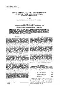
2. Problem formulation A finite rotor element is shown in fig 1. In real co-ordinates the element stiffness matrix [K], element translational mass matrix [MT], element rotational mass matrix [MR] and the element gyroscopic matrix [G] are (8x8) if one ignores the axial and torsional degrees of freedom. The matrices [K], [MT] and [MR] being the matrices for a 3d beam element are available in any standard text in finite elements [1] and the [G] is available in [2]. The equation of motion of the rotor in real co-ordinates is represented as ሺሾ‫ ்ܯ‬ሿ ൅ ሾ‫ܯ‬ோ ሿሻሼ‫ݔ‬ሷ ሽ െ ߗሾ‫ܩ‬ሿሼ‫ݔ‬ሶ ሽ ൅ ሾ‫ܭ‬ሿሼ‫ݔ‬ሽ ൌ Ͳ

(1)

Fig. 1. Finite rotor element

Here : represents the spin speed and {x} represents the displacement vector in real co-ordinates. If complex co-ordinates are used, the co-ordinates are defined by ‫ݖ‬ଵ ൌ ‫ݔ‬ଵ ൅ ݆‫ݔ‬ଶ ǡ߰ଵ ൌ ߮ସ െ ݆߮ଷ ‫ݖ‬ଵᇱ ൌ ‫ݔ‬ଵᇱ ൅ ݆‫ݔ‬ଶᇲ ǡ߰ଵᇱ ൌ ߮ସᇱ െ ݆߮ଷᇱ 

(2)

In complex co-ordinates the element stiffness matrix [K], element translational mass matrix [MT], element rotational mass matrix [MR] and the element gyroscopic matrix [G] are (4x4). The matrices [K], [M T] and [MR] being the matrices for a 2d beam element are available in any standard text in finite elements [1] and the matrix [G] is twice of [MR] as shown in [3]. For convenience the [G] is given here: ͵͸ ʹߤߢ ଶ ͵݈ ሾ‫ܩ‬ሿ ൌ ൦ ͵Ͳ݈ െ͵͸ ͵݈

͵݈ Ͷ݈ ଶ െ͵݈ െ݈ ଶ

െ͵͸ െ͵݈ ͵͸ െ͵݈

͵݈ െ݈ ଶ ൪ െ͵݈ ଶ Ͷ݈

Here N is the radius of gyration. It needs to be observed that [G] is now symmetric. Physically in complex co-ordinate, the rotor behaves as a 2d beam element in the complex plane. The equation of motion of the rotor in complex co-ordinates is represented as ሺሾ‫ ்ܯ‬ሿ ൅ ሾ‫ܯ‬ோ ሿሻሼ‫ݖ‬ሷ ሽ െ ݆ߗሾ‫ܩ‬ሿሼ‫ݖ‬ሶ ሽ ൅ ሾ‫ܭ‬ሿሼ‫ݖ‬ሽ ൌ Ͳ

(3)

Here {z} represents the displacement vector in complex co-ordinates. While this formulation reduces the problem size drastically, still full benefit of the formulation cannot be drawn as the Eigen value problem is Quadratic. If the spin speed to whirl speed ratio is taken as n (݊ ൌ ȳΤ߱) as proposed by [4], the Eigen value problem becomes ሾ‫ܭ‬ሿሼܼሽ ൌ ߱ଶ ൫ሺሾ‫ ்ܯ‬ሿ ൅ ሾ‫ܯ‬ோ ሿሻ െ ݊ሾ‫ܩ‬ሿ൯ሼܼሽ

(4)

Here ߱ represents the whirl speed and {Z} represents the eigen vector in complex co-ordinates. Equation (4) represents a simple eigen value problem. Further [G] merges with [M T] and [MR]. The analogy with a problem of structural dynamics is established.

400

Smitadhi Ganguly et al. / Procedia Engineering 144 (2016) 398 – 405

By this method, using different positive values of n, one can plot the backward branch of the campbell diagrams for different modes and using different negative values of n, one can plot the forward branch of the campbell diagrams for different modes. Now comes the question of lumping. As the analogy with a structural dynamic problem is established, naturally one would attempt to lump [MT], [MR] and [G]. The methods of lumping [MT] are well established and a nice discussion is given in [1]. Lumping of [MR] and [G] is the objective of the present work. Intuitive understanding is often the basis of lumping. Intuitive understanding of [M R] is easier than [G]. Since [G] is twice [MR], once [MR] is lumped, [G] will be automatically lumped. In the present work, lumping of [MT] and especially [MR] is discussed. Two possible simple but effective proposals of lumping [MT] in a 2d beam element are i) Lumping by putting half the mass at either node in the translational degrees of freedom and putting zero for the mass moment of inertia in the rotational degrees of freedom [1]. So [M T] becomes diag ሾΤʹ Ͳ Τʹ Ͳሿ. Here m is the mass of the beam element. ii) Lumping by putting half the mass at either node in the translational degrees of freedom and putting the moment of inertia of half of the element at either node in the rotational degrees of freedom [1]. So, [M T] becomes diag Τʹ ሾͳ Žଶ Τͳʹ ͳ Žଶ Τͳʹሿ It is relevant to consider the origin of [MT]. The translational kinetic energy of an elemental mass particle of the beam element is discretised by using the shape function of the beam and integrated over the element. This produces the consistent [MT]. Though the original energy is purely translational, the mathematical process produces coefficients in the rotational and cross coupled degrees of freedom. So, during lumping, it is a common practice to put zero in the rotational degrees of freedom as in option (i) above. Such a scheme often gives accurate Eigen values provided the discretisation is not too poor. In analogy with the above, the various proposals for lumping [MR] that are considered here are i) Calculating the mass moment of inertia of the prismatic element (square or circular cross section) about the centre of mass and lumping half of it at the rotational degrees of freedom at either node. For the translational degrees of freedom either half the mass may be used else zero. This process is not reasonable as unlike mass, moment of inertia is an axis dependant property. ii) The expression for mass moment of inertia of a prismatic element about an end is given as ݉Nଶ ൅ ᪞݈݉ ଶ . So it has two contributions - the first due to a prismatic thin disc and the second due to a thin rod. Here N is the radius of gyration of the prismatic thin disc. During lumping either the first effect or both may be considered. Further the coefficients in the translational degrees of freedom may be put to zero. iii) The proposal is same as that of the above but half the mass is used in the translational degrees of freedom. The origin of [MR] is the rotational kinetic energy of a thin elemental disc of the beam element. This energy is discretised by using the shape functions of the beam element and integrated to obtain the consistent [M R]. As before, the mathematical process produces entries at the translational and cross coupled degrees of freedom. So during the lumping process, in analogy with the lumping of [M T], it sounds logical to use zero in the translational degrees of freedom. Further since the original energy is due to the thin disc like effect, it also appears reasonable, to use the thin disc like component only of the moment of inertia of half the beam element in the lumping scheme. Accordingly the various proposals for lumping [M R] reduces to Calculating the mass moment of inertia of half the prismatic member and considering only the thin disc like component of the same. For the translational degree of freedom zero is used. So [M R] becomes diag ߤߢ ଶ Τͺ݈ ሾͲ Ͷ݈ ଶ Ͳ Ͷ݈ ଶ ሿ. Here ߤ is the mass per unit length of the beam. From the above discussion, two schemes are possible – i) Considering [MT] of proposal (i) and the above [M R] (referred as Proposal 1) ii) Considering [MT] of proposal (ii) and the above [MR] (referred as Proposal 2) If one goes by the observations stated above, the first proposal is expected to give better results.

Smitadhi Ganguly et al. / Procedia Engineering 144 (2016) 398 – 405

401

3. Numerical simulation Several combinations of approximating [MT] and [MR] has been numerically tried. As expected, only the above two proposals have yielded consistently good results. Among the two proposals, the first proposal is superior. Three examples have been chosen for elucidating the process of lumping. 3.1. Example 1 A simply supported square shaft of side 15 mm and a length of 600 mm is considered (fig. 2). A circular disc of radius 141.4 mm (Radius of gyration 100 mm) and mass 1 kg is placed at 2:1 point. The shaft has been discretised by using 4 elements (2 elements on either side of the disc), 6 elements (2 elements on shorter side of the disc and 4 on the longer side of the disc), 8 elements (4 elements on either side of the disc). Using this discretisation the 1 st and 2nd critical speeds (forward and backward) have been obtained. For the 1 stcritical speed 6 elements gives accurate results. For the 2nd critical speed 8 elements gives accurate result. For the 3rd and 4th critical speeds 12 elements (4 elements on shorter side of the disc and 8 elements on the longer side of the disc) has been used. The results obtained by either proposal of lumping are compared with the consistent mass method in Table 1. The agreement is good. The Campbell diagram for the 1 st and 2nd critical speeds using 6 elements have been plotted in figures 5 & 6.

Fig. 2. Simply supported single disc non-Jeffcott rotor having square cross-section

3.2. Example 2 A simply supported round shaft of diameter 15 mm and a length of 600 mm is considered (fig. 3). The circular disc size and position is same as in Example 1. An identical activity has been performed. The results follow a similar trend. The results are tabulated in Table 2. The Campbell diagram for the 1st and 2nd critical speeds has been plotted in figures 7 & 8.

Fig. 3. Simply supported single disc non-Jeffcott rotor having circular cross-section

3.3. Example 3 A simply supported round shaft of diameter 20 mm and a length of 600 mm is considered (fig. 4). Two circular discs same as in Example 1 has been considered. The disc are placed at the two 1/3 rd points. This is an example of a more complex rotor. The shaft has been discretised using 6 elements (2 elements for each section of the shaft – i.e., support to 1st disc, in between discs, 2nd disc to support) and 12 elements (4 elements for each section of the shaft). The 1st and 2nd critical speeds have been obtained using 6 elements. For the 3rd and 4th critical speeds 12 elements have been used. The results have been found to be accurate. The results are tabulated in Table 3. The Campbell diagram for the 1st and 2nd critical speeds has been plotted in figures 9 & 10.

Mode

4th

Mode

3rd

Mode

2nd

Mode

1st

Proposal 1

Proposal 2

2778.7

7883.0

8080.5

2405.1

2343.3

0

+1

+2

-1

-2

2323.5

2384.9

7017.3

6870.6

2757.2

919.4

6961.7

919.5

-2

1120.6

-2

1120.7

-1

2176.9

2078.9

7018.3

2194.5

+2

-1

2094.1

+1

1583.9

358.3

8894.3

1586.4

0

8748.4

358.4

-2

367.8

+2

367.9

-1

393.2

385.4

+1

393.2

+2

7158.6

385.4

+1

376.9

0

376.9

6960.9

7017.7

8821.1

8678.4

7158.5

2323.5

2384.8

7015.7

6867.8

2757.2

919.4

1120.6

2176.9

2078.8

1583.9

358.3

367.8

393.2

385.4

376.9

6921.3

6977.6

8818.9

8674.8

7117.3

2322.1

2383.4

6976.2

6830.1

2755.7

919.5

1120.6

2175.7

2077.8

1583.7

358.4

367.9

393.2

385.4

376.9

2232.2

2300.2

8357.5

8215.0

2743.8

912.9

1111.8

2068.6

1976.2

1551.9

361.1

370.7

396.0

388.3

379.8

6805.9

6855.6

8406.2

8292.3

6991.2

2319.9

2381.7

6824.6

6684.7

2759.9

919.8

1121.3

2172.2

2074.7

1584.6

358.3

367.8

393.2

385.4

376.9

6807.7

6857.5

8797.7

8657.2

6994.6

2321.1

2383.7

6828.1

6690.7

2763.3

917.4

1117.7

2170.4

2070.8

1577.6

359.0

368.5

393.9

386.1

377.6

6914.9

6971.0

8800.4

8657.5

7110.8

2321.9

2383.2

6967.8

6821.9

2755.9

919.5

1120.6

2175.4

2077.6

1583.7

358.4

367.9

393.2

385.4

376.9

2050.3

2109.6

4642.1

4568.9

2462.4

901.3

1088.0

1908.2

1827.1

1474.9

357.1

366.4

391.2

383.6

375.3

6216.9

6261.8

7756.9

7638.2

6381.7

2249.1

2310.0

6237.1

6108.7

2676.1

915.4

1112.8

2102.9

2008.8

1554.9

356.9

366.3

391.3

383.6

375.2

6220.0

6264.7

8512.1

8361.4

6386.5

2250.7

2312.6

6243.9

6122.9

2687.2

915.1

1112.7

2102.9

2008.4

1555.5

358.1

367.5

392.7

385.0

376.5

6730.9

6784.2

8531.6

8392.9

6919.5

2303.5

2364.8

6775.2

6633.1

2736.3

918.5

1118.8

2157.0

2060.1

1576.6

358.0

367.5

392.7

385.0

376.5

4 beam 6 beam 8 beam 12 beam 4 beam 6 beam 8 beam 12 beam 4 beam 6 beam 8 beam 12 beam elements elements elements elements elements elements elements elements elements elements elements elements

0

Ex. 1 n

Consistent

Table 1. Tabulated results of the square shaft fitted with a single disc (speeds are in rad/sec)

402 Smitadhi Ganguly et al. / Procedia Engineering 144 (2016) 398 – 405

Fig. 4. Simply supported two disc non-Jeffcott rotor having circular cross-section

4th Mode

3rd Mode

2nd Mode

Mode

1st

Ex. 2

7635.1 6060.4 6023.5

-1

-2

7533.6

+2

6152.3

+1

1979.6

2020.3

6059.0

5963.0

2267.0

711.7

871.3

1873.8

1793.8

1275.7

285.9

294.2

315.9

309.3

302.0

6 beam elements

0

1996.4

-2

6862.2

+1

2037.5

2284.9

0

6990.9

711.7

-2

-1

871.3

+2

1889.2

1807.4

+1

-1

1277.2

+2

285.9

0

315.9

+2

-2

309.3

+1

294.2

302.0

0

-1

4 beam elements

n

Consistent

6023.0

6060.0

7571.6

7472.2

6152.2

1979.6

2020.3

6058.0

5961.4

2267.0

711.7

871.3

1873.8

1793.7

1275.7

285.9

294.2

315.9

309.3

302.0

8 beam elements

5988.6

6025.3

7570.4

7470.1

6116.8

1978.4

2019.1

6023.6

5928.1

2265.7

711.7

871.3

1872.8

1792.8

1275.6

285.9

294.2

315.9

309.3

302.0

12 beam elements

1900.0

1944.2

7199.4

7101.1

2232.1

707.6

866.2

1784.1

1707.9

1257.8

287.8

296.2

317.8

311.2

304.0

4 beam elements

Proposal 1

5885.6

5917.8

7227.7

7146.0

6006.6

1976.4

2017.5

5897.1

5805.3

2267.7

711.9

871.7

1869.9

1790.1

1276.5

285.9

294.2

315.9

309.3

302.0

6 beam elements

Table 2. Tabulated results of the circular shaft fitted with a single disc (speeds are in rad/sec)

5886.7

5918.9

7553.7

7455.4

6008.4

1977.1

2018.6

5899.2

5808.8

2269.9

710.4

869.5

1868.8

1787.6

1271.8

286.4

294.7

316.3

309.7

302.5

8 beam elements

5983.0

6019.5

7555.2

7455.7

6111.1

1978.2

2019.0

6016.7

5921.3

2265.8

711.7

871.3

1872.5

1792.6

1275.7

285.9

294.2

315.9

309.3

302.0

12 beam elements

1748.4

1787.5

4011.4

3962.6

2025.5

700.5

851.3

1646.5

1579.0

1202.5

285.1

293.2

314.5

308.0

300.9

4 beam elements

Proposal 2

5377.8

5407.1

6674.7

6591.0

5486.3

1916.9

1957.4

5390.2

5305.9

2201.6

709.2

866.5

1811.5

1734.1

1256.3

285.0

293.1

314.6

308.1

300.9

6 beam elements

5379.7

5408.8

7317.0

7213.1

5488.9

1917.9

1958.9

5394.1

5314.2

2207.9

709.0

866.5

1811.4

1733.9

1257.1

285.7

294.0

315.6

309.0

301.8

8 beam elements

5823.4

5858.2

7328.3

7231.4

5946.9

1962.7

2003.4

5851.5

5758.5

2249.9

711.2

870.2

1857.1

1777.7

1270.9

285.7

294.0

315.6

309.0

301.7

12 beam elements

Smitadhi Ganguly et al. / Procedia Engineering 144 (2016) 398 – 405 403

Whirl speed (rad/sec) 390

385

380

375

370

365

360

355

350 0

280 200

0

100 400

200

300 600

400

500 800

600 1000

310

305

300

295

290

285

700

800

900

Whirl speed (rad/sec)

n=0.2 n=0.4 n=0.6 n=0.8 n=1 n=1.2 n=1.4 n=1.6 n=1.8 n=2 Consistent FW Consistent BW Proposal 1 FW Proposal 1 BW

Fig. 5.Campbell diagram for the first mode of example1

n=0.2 n=0.4 n=0.6 n=0.8 n=1 n=1.2 n=1.4 n=1.6 n=1.8 n=2 Consistent FW Consistent BW Proposal 1 FW Proposal 1 BW

1000

Spin speed (rad/sec)

Fig. 7. Campbell diagram for the first mode of example 2

Whirl speed (rad/sec)

Whirl speed (rad/sec) 315

395

1200

Spin speed (rad/sec) 0

0 500

500 1000

1000

4th Mode

3rd Mode

2nd Mode

Mode

1st

Ex. 3

1500

1500

3923.3

10149.3 10063.8 9599.0

0 +1

2000

2000 2500

2500 3000

2000

1800

1600

1400

1200

1000

800 3500

1600

1400

1200

1000

800

600

3000

-2

2340.9

2340.8

2340.0

2647.1

2645.3

2645.1

10391.0 10302.5 9791.5 -1

3944.0

1336.5

+2

3922.9

1335.6

1658.5 1335.7

1656.5 -2

9285.4

2666.9

1656.6

9751.0

2657.7

10216.8 10127.0 9623.3

9838.2

+1

1145.8

1303.4

1732.2

1635.1

1483.6

368.2

379.7

416.1

-1

2657.9

0

1145.5

1303.3

1734.3

1636.5

1484.0

368.2

379.8

416.1

+2

1145.5

-2

1636.6

+1

1303.3

1484.1

0

1734.5

368.2

-2

-1

379.7

+2

416.1

8597.3

2611.7

1137.7

1290.8

1707.0

1611.7

1464.7

367.0

378.4

414.4

402.3

3848.6

1329.2

1645.0

2340.6

2645.2

2314.6

2616.5

10279.1 9036.2

10042.4 8844.6

3924.2

1335.6

1656.6

10103.4 8914.3

9728.4

2658.1

1145.5

1303.3

1734.2

1636.4

1484.0

368.2

379.8

416.1

403.9

2334.7

2638.9

9959.7

9731.3

3908.2

1334.2

1654.0

9798.9

9434.2

2647.3

1143.6

1300.3

1727.5

1630.3

1464.7

367.9

379.5

415.7

403.5

391.4

-1

403.8

390.3

+2

403.9

391.7

403.9

391.7

+1

391.7

391.7

0

Proposal 2

6 beam 12 beam 6 beam 12 beam 6 beam 12 beam elements elements elements elements elements elements

Proposal 1

n

Consistent

Table 3. Tabulated results of the circular shaft fitted with two discs (speeds are in rad/sec)

404 Smitadhi Ganguly et al. / Procedia Engineering 144 (2016) 398 – 405

400

2200

n = 0.2 n = 0.4 n = 0.6 n = 0.8 n=1 n = 1.2 n = 1.4 n = 1.6 n = 1.8 n=2 Consistent FW Consistent BW Proposal 1 FW Proposal 1 BW

Spin speed (rad/sec) 4000

3500

4500

Fig. 6.Campbell diagram for the second mode of example 1

320

1800

n=0.2 n=0.4 n=0.6 n=0.8 n=1 n=1.2 n=1.4 n=1.6 n=1.8 n=2 Consistent FW Consistent BW Proposal 1 FW Proposal 1 BW

Spin speed (rad/sec)

4000

Fig. 8. Campbell diagram for the second mode of example 2

405

Smitadhi Ganguly et al. / Procedia Engineering 144 (2016) 398 – 405 420 1700

n=0.2 n=0.4 n=0.6 n=0.8 n=1 n=1.2 n=1.4 n=1.6 n=1.8 n=2 Consistent FW Consistent BW Proposal 1 FW Proposal 2 BW

400

390

380

370

360

0

200

400

600

800

1000

1200

Spin speed (rad/sec)

Fig. 9. Campbell diagram for the first mode of example 3

n=0.2 n=0.4 n=0.6 n=0.8 n=1 n=1.2 n=1.4 n=1.6 n=1.8 n=2 Consistent FW Consistent BW Proposal 1 FW Proposal 1 BW

1600

Whirl speed (rad/sec)

Whirl speed (rad/sec)

410

1500 1400 1300 1200 1100 1000

0

500

1000

1500

2000

2500

3000

3500

4000

Spin speed (rad/sec)

Fig. 10. Campbell diagram for the second mode of example 3

4. Conclusion The finite element based equations of a rotor has been cast using complex co-ordinates. This makes the [G] symmetric. Instead of obtaining the eigen values (critical speeds) for a fixed spin speed and then varying the spin speed, a fixed spin to whirl ratio is taken, the critical speed determined and then the ratio is varied to plot the Campbell diagram. This approach converts the quadratic eigen value problem to a simple eigen value problem. Now [G] becomes analogous to Mass matrix of structural dynamics. Next the Mass and Gyroscopic matrices are lumped so that they become diagonal and computational efficiency is further improved.

References [1] [2] [3] [4]

R.D. Cook, D.S. Malkus and M.E. Plesha, Concepts and Applications of Finite Element Method, John Wiley & Sons, New York, 1989 H.D. Nelson and J.M. McVaugh, The dynamics of rotor-bearing systems using finite elements, ASME J. Eng. Ind. 98(2)(1976): 593-600 G. Genta, Dynamics of Rotating Systems, Springer, New York, 2005 V . Ramamurti and A.R. Pradeep Simha, Finite element calculations of critical speeds of rotation of shafts and gyroscopic action of discs, J. Sound and Vibration, 117(3)(1987):578-582