enforced upon each element, the total number of degrees of freedom is only 2/3 of ... of freedom to constraints from 1 to 4/3, which makes the arrangement suit-.
COMPUTER METHODS IN APPLIED MECHANICS AND ENGINEERING 4 (1974) 153-177. © NORTH-HOLLAND PUBLISHING COMPANY
ON NUMERICALLY ACCURATE FINITE ELEMENT SOLUTIONS IN THE FULLY PLASTIC RANGE J.C. NAGTEGAAL *, D.M. PARKS and J.R. RICE Division o f Engineering, Brown University, Providence, R.L, U.S.A. Received 17 April 1974 Revised manuscript received 8 May 1974 It is often found that tangent-stiffness finite element solutions for elastic-plastic materials exhibit much too stiff a response in the fully plastic range. This is most striking for the perfectly plastic material idealization, in which case a limit load exists within conventional small displacement gradient assumptions. However, finite element solutions often exceed the limit load by substantial amounts, and in some cases have no limit load at all. It is shown that a cause of this inaccuracy is that incremental deformation fields of typical two and three-dimensional finite elements are highly constrained at or near the limit load. This is shown to enforce unreasonable kinematic constraints on the modes of deformation which assemblages of elements are capable of exhibiting. A general criterion for testing a mesh with topologically similar repeat units is given, and the analysis shows that only a few conventional element types and arrangements are, or can be made, suitable for computations in the fully plastic range. Further, a new variational principle, which can easily and simply be incorporated into an existing finite element program, is presented. This allows accurate computations to be made even for element designs that would not normally be suitable. Numerical results are given for three plane strain problems, namely pure bending of a beam, a thick-walled tube under pressure, and a deep double edge cracked tensile specimen. These illustrate the ~ffects of various element designs and of the new variational procedure. An appendix extends the discussion to elastic-plastic computation at finite strain.
1. Introduction In recent years, the finite element method has been employed for analysis of structures exhibiting elastic-plastic material behavior [ 1 ], and many successful applications have been made (see [2] for a comparison of possible forms of the required incremental analysis). However, with the application of the method, at least in its tangent-stiffness form, to problems of plane strain, axisymmetric, and three-dimensional problems, inaccurate results are often obtained. The problem is most clearly demonstrated for structures of ideally plastic material. Then a limit load exists which can sometimes be calculated exactly or bounded from above by the kinematical theorem, while the finite element solution often seems to exhibit no limit load at all, but rather a steadily rising load-displacement curve attaining values far in excess of the true limit load. Similarly, for strainhardening materials having typical values for the plastic tangent modulus of two or more orders of magnitude less than the elastic modulus, the finite element solution exhibits an artificially high terminal slope of the load-deflection curve in the fully plastic range. Later we shall see examples of this for a beam in pure bending and for a punch problem. In the case of a plane strain extrusion problem [3], when a bilinear constitutive law with slight plastic * Currently 570 Ordnance Regiment, Royal Dutch Army.
154
J.C Nagtegaal et al., On numerically accurate finite element solutions in the fully plastic range
work-hardening (d?/dgp --- H = 4.4 × 10 -3 E, where E is the Young's modulus) was incorporated, a finite element extrusion pressure of 1.5 times a slip-line solution (using the same yield stress as the linearly hardening model) was attained with overall billet displacements only of order six times the displacement obtained at the slip line limit load. This indicates that the computed stiffness in the fully plastic range far exceeds what would be expected for the small hardening modulus used. 1.4 1.2
i¢~ LIMIT LOAD
~ - ~ . - ~
O'NET I'0
/~'~MID ~/ ,~//
- LIGAMENT ~ LOADING F u LOADPOINT
~o o.s
CONSTANT END DISPLACEMENT uEND • uLOAOPOINT
0.6 0,4 0.2 O r '~.0
I
I.o
I
2.0
I
3.0
I
4.0
I
5~
I
6.0
I
7.0
I
8.0
i0
9
-"
EuLOAD POIN~O.Oh
Fig. 1. Load-displacement curves obtained from finite element solutions of plane strain single edge cracked tensile specimens subjected to mid-ligament loading and constant end displacement boundary conditions.
In some cases, however, the correct limit load is obtained. Fig. 1 illustrates some of the peculiarities which have been encountered by the authors and co-workers in elastic-perfectly plastic analysis of plane strain bodies containing cracks. The finite element meshes shown in fig. 2 were used to solve the single-edge notched plane strain tensile specimen subject to both uniform end displacement [4] (i.e., no end rotation) and the static equivalent of a mid-ligament concentrated force. These two loading conditions have the same analytical limit load, namely, twice the yield stress in shear on the net section. As can be seen in fig. 1, the overall load-deflection curves of the two loading conditions are quite different in the fully plastic regime. The solution for the midligament loading clearly indicates the correct limit load, while the constant end displacement solution exceeds the limit load, with the load continuing to rise at a roughly constant rate. A cause of these problems relates to the fact that the deformation state of an elastic-perfectly plastic material is highly constrained at limit load; for the usual material idealization, deformation increments at limit load will be strictly incompressible. In the usual finite element formulation, in terms of kinematically admissible displacement fields, the same condition will have to be satisfied. In particular, a tangent-stiffness finite element solution satisfies the incremental virtual work principle
f S
elem.
f % dVe em. ,
(1.1)
Velem"
precisely, where °ii is the stress rate following from the prescribed constitutive law in terms of the current stress oii and strain rate ~q within each element. This stress rate can be written as
J.C. Nagtegaal et al., On numerically aceurate finite element solutions in the fully plastic range
155
uEND
h
.I
[.
h
Fig. 2. Finite element meshes used to solve the mid-ligament loading and constant end displacement single edge cracked tensile specimens.
(1.2)
Oij ~- Sij d- 1 8i j Okk '
where ~,/is the deviatoric stress increment. Since the plastic deformation will be assumed purely deviatoric, the hydrostatic stress increment-~ agk can be expressed as bkk = h:ekk ,
(1.3)
where
= E/3( 1 - 2v)
(1.4)
is the elastic bulk modulus and gkk is the dilatational strain increment. Substitution of ( 1.2) and (1.3) in ( 1.1 ) then furnishes
f ',i,,dS = s
f
[sijeij + K(Ckk )2 ] dVelem" ,
(1.5)
elem. Velem.
where eij is the deviatoric strain increment. In the vicinity of the limit load, the term sii eq will tend to vanish pointwise, but, as follows from plastic normality, will never be negative. Hence, from (1.5), this implies that the incremental finite element solution satisfies
J.C. Nagtegaal et al., On numerically accurate finite element solutions in the fully plastic range
156
f~idS>~ elern. ~ f n(eke)2dVelem.. S
(1.6)
Velem"
The following result may thus be stated: In order for a limit load to exist for the discretized finite element model of an elastic-plastic problem, it is necessary that the elements be capable of deforming so that ~kk = 0 pointwise throughout the elements. Otherwise (1.6) requires that the load-deflection curve be steadily rising - i.e. no limit load exists. In the next section it will be shown that, except for plane stress problems, the requirement ekk = 0 severely constrains the class of deformations of which typical finite element grids are capable. When they are forced to deform in such a constrained fashion, unreasonably high limit loads, or no limit loads at all, will result. On the other hand, even if no limit load is achieved in the finite element formulation, it is to be expected (and is indeed observed) that the slope of the load-deflection curve is reduced substantially from its initial elastic value at load levels near the theoretical limit load. This, however, does not allow an accurate inference of the limit load. Even if the material is linearly work-hardening with a small hardening coefficient, the terminal slope of the load-deflection curve will not necessarily be accurately determined (as was argued previously and will be demonstrated in an example), since the material will deform in a nearly incompressible fashion in the fully plastic range. It is clear that the problems discussed here have a strong similarity to problems encountered in the analysis of incompressible fluids and rubber-like solids. The difference is that the material behaves incompressibly only as limit conditions are approached because the effective shear modulus then tends to vanish, whereas fluids and rubber-like solids behave incompressibly from the start because the bulk modulus is very large. The essential problem is the same in both cases, however, in the sense that the incompressibility requirement puts too severe constraints on the possible deformation modes.
2. Analysis In the previous section, it has been observed that elements must be capable of deforming without change of volume pointwise if a limit load is to be obtained. It is therefore useful to investigate the constraints this enforces upon each element, and the effect of these constraints on the behavior of an assemblage of elements. Consider, for instance, the grid of 4-node rectangular isoparametric elements shown in fig. 3. Within each element, the displacement increments are of the form
,itx}
it= litv =a+bx+cy+dxy,
(2.1)
where the vectors a, b, etc. are expressed in terms of the nodal velocities and coordinates. Now, the incompressibility constraint for plane strain has the form
J.C. Nagtegaal et al., On numerically accurate finite element solutions in the fully plastic range
aft x bhy Cxx + ~yy = ax + ay = 0 ,
157
(2.2)
and this requires that d = 0 as well as that b x + ¢y = 0, a total of three constraints. The fact that d = 0 means that at limit load each element has strain increments which are constant throughout the element. It is then evident from displacement continuity that all elements marked * in fig. 3 must have the same value of ~xx, whereas all elements marked t must have the same value of Cyy. Moreover, since ~ = - ~yy, ~xx and ~yy will be the same in all elements marked • or ?. Since a similar argument can be set up for any row and column, e:cx and eyy must be the same in every element o f the grid. Clearly, this is a very unrealistic constraint.
t
t
t
*tt
t
m
YT
!
~-x
Fig. 3. Propagation o f incompressibility constraints in a mesh of rectangular four-node isoparametric plane strain finite elements.
It is at least possible for this mesh to have a non-uniform shear ~xy, but the situation is even worse in case the grid consists o f arbitrary quadrilateral isoparametric elements. Within an element the displacement increments are of the form = a + br/+ c~ + dr/~,
(2.3)
where r/and ~ are defined by {y} = a t +
pr/+Y~+&r//j.
(2.4)
(See, for instance, [6].) A lengthy but straightforward calculation furnishes the three incompressibility constraints per element: b x ~ y - Cx~y - by'}' x + Cy~x = 0 , b x ~y -- d x ~ y -
by~ x + dyfl x = O,
d x T y - e x ~ y - dy')' x + Cy6 x ~- 0 .
(2.5)
158
J.C. Nagtegaal et al., On numerically accurate finite element solutions in the fully plastic range
A solution to this system of equations in terms of three parameters A, B, and C is b x = A 13x + B ~ y ,
b y = (?(ix - A ~ y ,
Cx = A Y x + g " / y ,
cy = C'y x - A'),y ,
d x = A 8 x + BS>, .
dy = C6 x -- A 6y .
(2.6)
Substitution of (2.6) in (2.3) then makes it possible to eliminate r/and ~ from (2.3) and (2.4) this furnishes the displacement increments -
hx = D + A x
+By,
@ = E + Cx - Ay
,
(2.7)
where the constants D and E do not depend on A, B and C. Hence, if the incompressibility constraint is to be satisfied, the strain increments will be constant throughout the element.
A 8
Fig. 4. Mesh of arbitrarily skewed four-node isoparametric plane strain finite elements.
This has catastrophic effects for an arbitrary grid. Consider, for instance, the grid in fig. 4, and specify the displacement increments of the three nodes A, B and C. Because the displacement increments of nodes A and B define the extensional strain along AB in element I, and because the element must deform with a constant strain of zero dilatation, we must then specify the component of displacement increment of node E in the direction normal to AB. Similarly, because the displacement increments of nodes B and C determine the extensional strain along BC in element I1, we must also specify the displacement component of node E in the direction normal to BC. The incompressibility constraints of elements I and II then specify the components of displacement increment of node E in two linearly independent (though not orthogonal) directions. Thus the displacement increment vector of E is fully determined, and, in fact, it corresponds to that increment which causes identical strain increments in elements I and II. The displacement increments of nodes D and F are then also determined. Continuation of the argument then furnishes that the strain increment will be constant throughout the grid. It should be noted that this argument holds only if the element boundaries do not form a straight line through the body; over such a line the shear strain increment can be discontinuous.
J.C. Nagtegaal et aL, On numerically accurate finite element solutions in the fully plastic range
159
Examples of the unreasonable constraints enforced by pointwise incompressibility upon displacement increment fields of other two and three-dimensional mesh configurations are given in Appendix 1. We are now in a position to explain the results of fig. 1, bearing in mind a result of perfectlyplastic limit analysis: namely, that while the limit load is unique, the deformation field at limit load need not be unique. An acceptable limit field for both loading conditions, giving the correct limit load, is that of concentrated deformation on 45 ° lines from the crack tip to the surface, as shown in fig. 5a. An alternative limit field for the mid-ligament loading is shown in fig. 5b. This field consists of constant strain increments within the region bounded by the two 45 ° lines from the crack tip. The rest of the body is rigid, so the overall effect is that of a rotation of the two rigid regions about the crack tip. In fact, this was exactly the velocity field obtained at limit conditions in the finite element solution of the mid-ligament loading problem. Since the deforming regions do so uniformly, and the 45 ° lines coincide with element boundaries, thd mesh of focused isoparametric quadrilaterals could readily accommodate the incompressibility constraints, hence leading to a very accurate finite element prediction of the limit load. In contrast, however, the rotation produced by this field is incompatible with the constant enddisplacement boundary condition of the other loading. The same constant strain pattern cannot develop, and an ever-worsening overestimate of the limit load results.
r" . . . . . . .
45 °
45* ".-- (~X X s
i. .
.
.
.
.
.
- ~yy = CONST.
J
F (a)
(b)
Fig. 5a. Acceptable limit mechanism for plane strain single edge notched tensile specimen subject to either mid-ligament loading or constant end displacement, b. Alternative limit mechanism for mid-ligament loading.
Although the problem has now been analyzed sufficiently for four-noded isoparametric quadrilateral elements, a more systematic approach is needed to find a solution to it. It is therefore useful to consider the matter of convergence of the solution if the mesh is refined. Refinement of the mesh will have two opposing effects: 1) It will increase the number of nodes, and since each node represents a specific number of degrees of freedom, it will increase the total number of degrees of freedom. 2) On the other hand, it will increase the number of elements, and since each element has a certain number of incompressibility constraints enforced upon itself, it will increase the total number of constraints. It is clear that convergence will occur only if the total number of degrees of freedom increases
160
J.C. Nagtegaal et al., On numerically accurate finite element solutions in the fully plastic range
faster than the total number of constraints. This furnishes a relatively simple criterion to check whether a mesh of a certain type will be adequate to furnish accurate limit loads and flow fields. It should be noted that the total number of constraints is not always equal to the number o f elements times the number of constraints per element. Sometimes elements can be arranged such that the constraints are no longer independent, an important example of which will be discussed in the next section. For the moment, however, these special cases will not be considered.
Fig. 6. Nodal angles for a linear strain triangular finite element.
It is thus important to determine the ratio o f the total number of nodes to the total number of elements in the grid when it is refined. Consider a body, loaded in plane strain, the crosssection of which is subdivided into a mesh o f elements o f identical type. Define the nodal angles 07 o f an element a as the inner angle formed at the node by the two adjacent element boundaries. For each type o f element the sum o f these nodal angles is a given number. Consider, for instance, the six-noded triangle of fig. 6. Each of the nodal angles at the mid-points o f the sides is equal to 7r radians, whereas the sum of the angles 0F, 0 F and 0 3 is also equal to 7r radians. Hence the sum of all nodal angles is equal to 47r radians. Similarly simple calculations can be made for other types of elements. For generality, let us assume that the sum o f the nodal angles of a particular element type is equal to nlr radians. If the grid consists of p elements, then the sum o f all nodal angles of all elements is equal to ~ ] 0'~ = p n n
.
(2.8)
i
The sum of all nodal angles can also be calculated in a different way. Suppose the mesh has k nodes inside the body and l nodes on the boundary. The sum of the nodal angles around each interior node is equal to 27r radians, whereas the sum o f the nodal angles at a boundary node is equal to ~r-7 radians, where "y is a small angle due to the curvature o f the boundary. In this way the sum is readily calculated as ~ 0 ~
= ( 2 k + l + 2c - 4 ) r r ,
(2.9)
c~ i
where c is the degree o f connectivity of the body (c = 1 if simply connected, etc.). From (2.8) and (2.9) then follows the equality
J.C. Nagtegaal et al., On numerically accurate finite element solutions in the fully plastic range
pn = 2 k + l + 2c - 4 ,
161
(2.10)
or, alternatively, p=2+ k
n
l
2c-4
-~
nk
(2.11)
Now if the mesh is refined, p, k, and I will all increase; hence the last term will vanish. Moreover, if the mesh is refined uniformly, k (the number of interior nodes) will increase approximately as the square of I (the number of boundary nodes). Hence
,ira k-~=
-n"
(2.12)
Consider what this means for a grid of isoparametric quadrilateral elements. The sum of the nodal angles in one element is equal to 27r radians, and hence n = 2. Substitution in (2.1 2) then furnishes that in the limit the number of nodes will become equal to the number of elements. Since each node represents two degrees of freedom, and three incompressibility constraints are enforced upon each element, the total number of degrees of freedom is only 2/3 of the total number of constraints. Hence convergence will not in general occur, which reaffirms the previously obtained result. Similar derivations can be made for other planar elements as well as for axisymmetric elements since (2.12) holds as well for this class. The results are displayed in table 1. The range of value of constraints per element from 6 to 8 given for the 8-noded quadrilateral depends on whether the sides of the element are linear or quadratic, respectively. For three-dimensional elements, however, the ratio of nodes to elements is not unique, since the sum of the solid angles of a polyhedron is not a constant. Therefore one has to determine this ratio for a specific arrangement of elements. For some common regular grids, and thus of any grid which is equivalent, the results are displayed in table 2. It may be assumed that these results are fairly representative for most common types of arrangements. The results in tables 1 and 2 indicate that none of the usual finite elements, except the 6-noded plane strain triangle and, to a much lesser degree, the 10-noded tetrahedron, is adequate to analyze (approximately) incompressible, and thus limit load, behavior. Before going into a more systematic approach to solve the problem, let us consider what can be obtained by a special arrangement of the elements.
3. Special arrangements of elements As has been mentioned previously, the total number of constraints is not necessarily equal to the product of the number of elements and the number of constraints per element. For special arrangements of elements, the total number of constraints may be less than this product. The obtained improvement, however, will be small, since it is necessary to combine a number of elements to eliminate one constraint. Thus this method will work only for elements for which the ratio of degrees of freedom to constraints in tables 1 and 2 is close or equal to one.
162
J.C. Nagtegaal et al., On numerically accurate finite element solutions in the fully plastic range
Table 1 The effectof meshrefinementon the ratio of total degreesof freedomto total numberof incompressibilityconstraintsfor some commontwo-dimensionalfiniteelements.
Element Type
Constraints
~
I
Ratio
112
1
Element Elements Constraints
constant s t r a i n triangle
"~
Ratio Nodes
4-node
2/3
quadrilateral
IP
~
linear s t r a i n
4/3
~Tia~gle 8-node
quadrilateral
6¢o8
to 3/~
i/2
i/3
2/s
>. 9
.< 213
Consideration of tables 1 and 2 with this in mind indicates that only a few types of elements could possibly be used for this purpose: for plane strain, the 3-noded triangular element and perhaps the 8-noded quadrilateral element, and for three-dimensional problems, the 10-noded tetrahedron. None of the axisymmetric elements could possibly be used. As yet the only successful arrangement that has been discovered is the combination of four 3-noded triangles as shown in fig. 7. Note that the triangular element boundaries form a quadrilateral "element" and its diagonals. This combination has the special property that if the incompressibility constraint is satisfied in three of the elements, the constraint in the fourth element is automatically satisfied. This brings the ratio of degrees of freedom to constraints from 1 to 4/3, which makes the arrangement suitable for analysis near limit load. The proof of this special property is given below.
1C. Nagtegaal et al., On numerically accurate finite element solutions in the fully plastic range
163
Table 2 The effect of mesh refinement on the ratio of total degreesof freedom to total number of incompressibilityconstraints for some common arrangements of three-dimensionalfinite elements.
Element Type and Amrangement
5 ¢ o n s t a n ~ s~rain t e t r a h e d r a in cube; cubes in r e g u l a r lattice
~ ,~ i , -~
~
~_qk N~ -~
~
, ,
Constraints Element
Ratio Nodes Elements
De~.Freedom
:].Is
3/5
8-node isoparamezric cubes in ,regular l a t t i c e 5 linear strain t e t r a h e d r a in cube; cubes in regula~ l a t t i c e
~
Ratio Constmaints
3/7
7/5
4
2Z/20
20-node
~L
ltsop~ametri ¢ icubes in ~
>. 16
.< 31~
''~ ' regulaz'
~--
lattice
4
2
Fig. 7. Four constant strain triangular finite elements arranged to form a quadrilateral and its diagonals. Let the c o o r d i n a t e s o f the n o d e i be xi, and let the n o d e have a d i s p l a c e m e n t i n c r e m e n t h i. T h e area A o f e l e m e n t I b e f o r e the displacement i n c r e m e n t has t a k e n place is t h e n equal to A = ~ [ ( x u - X o ) X (x I - X o ) ] " k ,
(3.1)
164
Z C. Nagtegaal et al., On numerically accurate finite element solutions in the fully plastic range
where × and • denote the usual vector and scalar products respectively, and k is the unit vector perpendicular to the plane of the elements. Similarly one finds that after the displacement increment has taken place, A + A =-~[(x2+/t 2 - x o - / t o) × (x 1 +/t I - X o - / t o ) ] . k .
(3.2)
Subtraction of (3.1) from (3.2) furnishes = 3 [(X2 -- X O) X (/t I -- /tO) -- (,X"1 -- XO) X (/t 2 - - / t o ) + (/t 2 - - / t o ) X (/t 1 - - / t o ) ] • k .
(3.3)
When one neglects the second order terms, the incompressibility constraint takes the form (x 2 - X o ) × (/t I - / t o ) = (x 1 - X o ) × (/t z - / t o ) .
(3.4)
Similarly, for the elements II and III, one obtains (x 3 - X o ) × (/t 2 - / t o ) = (x~ - X o ) × (/t 3 - / t o ) ,
(3.5)
(x a - x o) × (/t 3 - i t o) = (x 3 - x o) X (/t a - i t o) .
(3.6)
Now multiply (3.4) by Ix s - x o I/Ixl
- Xol, furnishing
Ix3 - Xo I Ix1 - X o l (x 2 - X o ) × (/t I - / t o ) = - (x 3 - X o ) × (/t 2 - / t o ) ,
(3.7)
since x 3 - x o and x 1 - x o have opposite directions. Similarly, one obtains for (3.6) Ix 2 - X o l - ( x 2 - x o ) X (it 3 - / t o) - [xa Xo((X3-Xo)
X (it a-~to).
(3.8)
Substitution of (3.7) and (3.8) in (3.5) then furnishes ]X 3 - - X o [
IX 2 - - X o
Ix1 - X o l (x 2 - x o ) × (/t 1 - / t o ) - I x 4 - X o (x 3 - x o ) × (/t 4 - 1 t o ) ,
(3.9)
or, alternatively, IX 4 --XOI
Ix2-Xol(X 2-xo )×(/tl-lto)=ix
IX 1 - - X 0
3-x°
(x 3 - x o ) × ( / t 4 - 1 t o ) .
With the same argument as was used for (3.7) and (3.8) this yields (x 4 - x o) x (/t I - / t o) = ( x I - x o) × (/t 4 - / t o) , which proves that the incompressibility constraint in element IV is satisfied.
(3.10)
Z C. Nagtegaal et d., On numerically accumte finite dement solutions in the fully plastic range
165
It should be noted that this approach requires no modification of existing finite element programs. The groups of four elements have all the generality in application of the usual quadrilateral elements, and the calculations can be carried out without changes to an already existing program. The principal shortcoming Of the method is that it can be applied only to problems of plane strain, for which another alternative (the 6-noded triangular element) already exists. Even this alternative can be slightly improved by arranging the 6-noded elements similar to the 3-nodes ones. The ratio of degrees of freedom to constraints then improves from 4/3 to 16/11. It should also be noted that the degrees of freedom available need not actually be incorporated into the finite element solution. For example the degrees of freedom corresponding to the interior node "0" of fig. 7 may be "condensed out" of the master stiffness matrix and recovered later. (See, for example, [7].) As yet no method has been devised to arrange the 10-noded tetrahedra such that an acceptable ratio of degrees of freedom to constraints is obtained. Therefore a different, more general approach is needed to solve problems other than those of plane strain.
4. A modified variational principle It has been discussed before that an absolute requirement for the existence of a limit load is that the dilatation increment ~kk vanishes pointwise. It has also been demonstrated that only a few of the conventional element types are, or can be made, useful to analyze problems under this constraint. Therefore it is desired that different elements be constructed for which fewer constraints per element are sufficient to satisfy the incompressibility requirement. This goal can be obtained by taking care that the dilatation is governed by fewer parameters than in the conventional elements. Clearly, this procedure may be applied only to higher order elements for which the conventional number of constraints per element exceeds unity. Theoretically it is possible to construct interpolation functions that have this property; in fact, if the arrangement in fig. 7 is taken as a single element, and the displacement of node 0 is chosen such that the dilatation in all subelements I through IV is the same, one has obtained such a function. This special field must, however, be considered as a "lucky guess", and a general approach to construct similarly simple fields for other elements does not seem to exist. An alternative way to solve the problem is to create a variational principle in which the dilatational strain increment and the displacement increments are present as independent variables. We then have complete freedom to characterize the dilatation by as many (or as few) parameters as we choose. Such a variational principle is akin to the Hellinger-Reissner principle [8], which admits the displacements and the stresses as independent variables. The validity of the present principle will, however, be proved here independently of the H - R principle. Consider the functional (4.1) V
where
ST
166
J.C. Nagtegaal et al., On numerically accurate finite element solutions in the fully plastic range •
--
1
"
+"
1
"
eij =-~(ui, j uj, i) ---~6ijUk. k is the deviatoric strain increment, W'(ki]) is the deviatoric rate potential • [W , =~siieii; 1 • • 6W , = si]6eii], • • • q~ is the (independent) dilatational strain increment, is the (instantaneous) bulk modulus. This functional is well defined if a finite bulk modulus ~: exists. That this functional corresponds to a valid variational principle is readily proved in the usual way. By taking the first variations in h i and ~ one finds
81= f (jijSkij+4;Sh,k)dV- f V
dSr+
ST
(4.2) V
and since
ai] = Jii + ~ 6 i i ,
(4.3)
this can be written (4.4) V
ST
V
The first two terms express the virtual work principle and hence imply that hi~ satisfy the continuing equilibrium equations in V and force rate.boundary conditions on S T in the usual manner. The last term provides the additional result that ~b = Uk,kIt is appropriate to compare the present principle with the principle created by Herrmann [5] for the analysis of incompressible, linear elastic materials. The functional used by Herrmann would have the incremental form H : H [ h , / ~ ] = f P[4,]~ii + 2V/~kk -- U(1--2V)/~ 23 d V V
f
7~ih, d S v ,
(4.5)
ST
where p is the shear modulus, u is Poisson's ratio, and where the "mean pressure function" is given by fl --
O kk
2/a( 1 +u) "
(4.6)
Apart from its specialization to linear elasticity, the fact that ~kk enters Herrmann's principle quadratically is an essential difference. Indeed, this does not allow for it the same simple procedures that can be based on the present principle and that allow the easy adaption of existing conventional stiffness programs to it. Before going to the application of the principle, let us determine how many constraints per element would be desired, in order to get an as close as possible approximation to continuum behavior. In the continuum, each material point represents two (in problems of plane strain or axisymmetric problems) or three (in three-dimensional problems) degrees o f freedom. For incompressibility, one constraint is valid at each material point. Hence the ratio of degrees of freedom to constraints in the continuum is equal to two or three, depending on the type of problem.
J.C. Nagtegaal et aL, On numerically accurate finite element solutions in the fully plastic range
167
It seems plausible that a finite element solution to an elastic-plastic problem would give the best overall approximation if the ratio degrees of freedom to constraints would be the same as in the continuum. Hence a "two" would be desired in the last column of table 1 and a "three" in the last column of table 2. This readily leads to a desired number of constraints per element. For instance, for the 4-noded quadrilateral elements in table 1, the desired number would be one, and for the 8-noded quadrilateral elements, it would be three. Similarly, for the 8-noded cube in table 2, one constraint would be desired. Similar desired numbers can be obtained for the other elements in the tables. Now let us for the moment restrict the discussion to those elements for which the desired number of constraints is equal to one. As has been discussed before, one then needs a dilatation increment governed by a single parameter. It is, on the other hand, necessary for convergence that at least a constant dilatational strain increment be obtainable within an element (see, for instance, [7]). Hence, it is necessary to choose in an element a (4.7)
¢ = Ca = constant. Substitution of (4.7) in (4.1) then furnishes P
1= ~ f [W'(kij)+K¢~itk,k-~K~]dV ~ - f 7"ifxidSr . ~=1
V~
(4.8)
ST
Variation of ¢~ then yields the relation
f
f ,