On Models for Complex Spatio-Temporal Point

On Models for Complex Spatio-Temporal Point Process Data

By: Morteza Raeisi

Supervisors: Edith Gabriel Florent Bonneu

A thesis submitted for the degree of Master of Mathematics and Applications (M2) (with Honours) in Probability and Random Models of Sorbonne University

Paris September, 2018

2

Contents Preface

5

1 Introduction 1.1 Spatial point processes . . . . . . . . . . . 1.1.1 First and Second-order properties . 1.2 Spatio-temporal point processes . . . . . . 1.3 Empirical and mechanistic models . . . . 1.3.1 Empirical models and methods . . 1.3.2 Mechanistic models and methods . 2 Spatio-temporal forest fire modelling 2.1 Modelling approach . . . . . . . . . . 2.2 Estimation approach . . . . . . . . . 2.2.1 Classical methods . . . . . . 2.2.2 Bayesian methods . . . . . .

. . . . . .

. . . . . .

. . . . . .

7 7 9 12 15 16 17

with point processes . . . . . . . . . . . . . . . . . . . . . . . . . . . . . . . . . . . . . . . . . . . . . . . . . . . . . . . .

. . . .

. . . .

19 19 23 23 24

. . . . . . . . .

. . . . . . . . .

27 28 29 32 32 33 34 35 38 40

. . . . . .

. . . . . .

. . . . . .

. . . . . .

. . . . . .

. . . . . .

. . . . . .

. . . . . .

3 Space time non-separable point process models 3.1 First-order separability . . . . . . . . . . . . . . . . . . 3.2 Second-order separability . . . . . . . . . . . . . . . . . 3.3 Non-separability in random field models . . . . . . . . . 3.3.1 Bochner’s Theorem . . . . . . . . . . . . . . . . . 3.3.2 Cressie-Huang representation . . . . . . . . . . . 3.3.3 Fully symmetric, stationary covariance functions 3.3.4 Positive and negative non-separability . . . . . . 3.4 Link between geostatistics and point process models . . 3.5 Non-separability in point process models . . . . . . . . .

. . . . . .

. . . . . . . . .

. . . . . .

. . . . . . . . .

. . . . . . . . .

4 Point process models taking into account multi-scale structures 4.1 Single-scale structures point processes . . . . . . . . . . . . . . . 4.1.1 Point patterns in space . . . . . . . . . . . . . . . . . . . 4.1.2 Point patterns in space-time . . . . . . . . . . . . . . . . . 4.2 Multi-scale structures point processes . . . . . . . . . . . . . . . 4.2.1 The types of interaction in space and time . . . . . . . . . 4.2.2 Models formulation . . . . . . . . . . . . . . . . . . . . . .

3

43 43 43 45 54 55 56

4

CONTENTS

Preface The spatio-temporal behaviour analysis is fundamental in areas such as environmental sciences, climate prediction and meteorology, epidemiology, image analysis, agriculture, seismology and astronomy, and so spatio-temporal point processes, rather than purely spatial point processes, must then be considered as potential models. Environmental phenomena can be modelled as stochastic point processes where each event, e.g. the forest fire ignition point, is characterised by its spatial location and occurrence in time. Additionally, information such as burned area, ignition causes, landuse, topographic, climatic and meteorological features, etc., can also be used to characterise the studied phenomenon. Thereby, the space-time pattern properties represent a powerful tool to understand the distribution and behaviour of the events and their correlation with underlying processes. Many measures describing the space-time distribution of environmental phenomena have been proposed in a wide variety of disciplines. We review them in this report. The main objective of this report is to give a state of the art to overcome unsolved methodological problems in the characterisation of spacetime patterns, in particular, the forest fire occurrences. In Chapter 1, we present a theoretical framework of spatial and spatiotemporal point processes as a mathematical tool for dealing with the concepts shown along the next chapters of this report. In Chapter 2, we review some articles in forest fires modelling and estimating with spatio-temporal point processes. In order to understand and model the stochastic mechanisms of spatiotemporal interaction, it is necessary to consider a non-separable framework. In Chapter 3, first, we investigate the non-separability in random field models and classes of the positive and negative non-separable stationary covariance models. Classifying models with respect to the type of non-separability help in choosing a more suitable class of models for the data. Finally, we investigate the nonseparability in point process models. Since little research has been published for point processes in non-separable framework, we discuss that the connections between point process and geostatistics are closest when the assumed model is the linear Gaussian model. In Chapter 4, we investigate the structures in spatial and spatio-temporal point process by visualization and analysis approachs. In more details, we investigate space-time clustering and interaction. We also propose some develop5

6

CONTENTS

ments in the context of spatial and spatio-temporal point process analysis with emphasis on the description of complex interaction structure between events. Multi-scale processes can be constructed easily by using hybridization. We investigate hybrid of Gibbs models in space and area-interaction point process in space and space-time as two empirical models in multi-scale structures point process. The main characteristics of hybrid of Gibbs models is that it is possible to describe the multi-scale interaction between the points in presence of larger scale inhomogeneity.

Morteza Raeisi September, 2018

Chapter 1

Introduction Random process models for space-time data play increasingly important roles in various scientific disciplines; among them are environmental science, agriculture, climatology, meteorology, and hydrology. This chapter gives an informal introduction to spatial point processes and spatio-temporal point processes.

1.1

Spatial point processes

Spatial statistics has been one of the most fertile areas for the development of statistical methodology during the second half of the twentieth century. A striking, if slightly contrived, illustration of the pace of this development is in Cressie (1993). Cressie established a widely used classification of spatial statistics into three subareas: geostatistical data, lattice data, spatial patterns (meaning point patterns). Within this classification, geostatistical data consist of observed values of some phenomenon of interest associated with a set of spatial locations xi : i = 1, ..., n, where, in principle, each xi could have been any location x within a designated spatial region. Lattice data consist of observed values associated with a fixed set of locations xi : i = 1, ..., n, that is, the phenomenon of interest exists only at those n specific locations. Finally, in a spatial pattern the data are a set of spatial locations xi : i = 1, ..., n presumed to have been generated as a partial realisation of a point process that is itself the object of scientific interest. Almost 20 years later, Gelfand et al. (2010) used the same classification but with a different terminology focused more on the underlying process than on the extant data: continuous spatial variation, discrete spatial variation, and spatial point processes. With this process-based terminology in place, continuous spatial variation implies a stochastic process, discrete spatial variation implies only a finite-dimensional random variable, and a point pattern implies a counting measure (Diggle et al., 2013). 7

8

CHAPTER 1. INTRODUCTION

Point process A point process is a collection of points randomly located on a Polish space. Point processes can be used as mathematical models of phenomena or objects representable as points in Polish space. Examples include locations of trees in a forest stand, blood particles on a glass plate, galaxies in the universe, and particle centers in samples of materials. Being based on this data structure, point process theory forms part of spatial statistics. So how is the analysis of spatial pattern data usually approached ? A simple graphical representation of the pattern of objects as a point map is a very useful preliminary step towards understanding its properties. We will discuss about it in Chapter 4 with more detail. This section provides the fundamental theory of point process. A point process is denoted by N. For a Borel set B ⊂ W ⊂ Rd , W is a d-dimensional window or the whole of Rd , but it could also be e.g. the (d1)-dimensional unit sphere and N (B) is the random number of points in B. It is assumed that N (B) < ∞ for all bounded sets B, i.e. that N is ‘locally finite’. The simplest point pattern exhibits complete spatial randomness (CSR), a property under which point locations occur independently and uniformly over B. In classical statistics, mean values are a fundamental concept. This is similar in the context of point processes, where mean numbers in fixed sets are particularly important. The value N (B) for a set B is a random variable and, if B is bounded, it makes sense to consider the mean E(N (B)), where E is the symbol for expectation. Thus E(N (B)) = Mean number of points of N in B.

(1.1)

Clearly, this mean depends on the set B, and it is therefore a (deterministic) function operating on sets (more precisely, a measure). Therefore, the notation Λ(B) = E(N (B)) is used and Λ is called the intensity measure. Under some continuity conditions, which are usually satisfied in practical applications of point process, a Rdensity function λ(B) exists that is called the intensity function with Λ(B) = B λ(x)dx. Motion-invariant A point process N is called stationary if N and the translated point process Nx have the same distribution for all translations x. This is written as N = Nx in distribution where Nx is the point process resulting from a shift of all points of N by the same vector x; if N = {x1 , x2 , ...} then Nx = {x1 + x, x2 + x, ...}. A point process N is called isotropic if N = {x1 , x2 , ...} and any rotation of it Rα N = {Rα x1 , Rα x2 , ...} have the same distribution for all α where Rα is a rotation operator. A point process that is both stationary and isotropic is called motion-invariant. A point process is called homogeneous (or first order stationary) if its intensity function is constant, otherwise it is said to be inhomogeneous.

1.1. SPATIAL POINT PROCESSES

9

Poisson process There exist various parametric point process models, and the simplest and most fundamental one is the Poisson process. A point process N on W is a Poisson point process with intensity function λ if the following properties are satisfied • For some λ > 0, and any finite planar region A ⊂ W , N (A) follows a Poisson distribution with mean λ|A|, • Given N (A) = n, the n events in A form an independent random sample from the uniform distribution on A, • For any two disjoint regions A, B ⊂ W , the random variables N (A) and N (B) are independent. Due to its property of complete spatial randomness, Poisson process is often treated as a baseline for detecting clustering or inhibition patterns. We will discuss about it in Chapter 4 with more detail. Marked point process As an important type of point process, marked point pattern analysis studies ensembles of objects scattered in space, but the objects are characterized not only by their positions but also by marks, i.e. additional data on each individual object, which may be either quantitative (continuous) or qualitative (discrete or categorial). Marked point process is a key method in spatial statistics as it analyses data consisting of observations of variables given at irregularly distributed points. These processes are models for random point patterns where marks that describe properties of the objects represented by the points are attached to the points. In other words, a marked point process M is a sequence of random marked points, M = {[xn ; m(xn )]}, where m(xn ) is the mark of the point xn . The points and marks in a marked pattern are often correlated. Consider, for example, data from a plant community where the points are plant locations and the marks plant size characteristics. In areas of high point density the marks may tend to be smaller than in areas with low point density resulting from stronger competition for limited resources. We can define the stationary, isotropy and intensity function similar to non-marked point process.

1.1.1

First and Second-order properties

In this section, we consider various theoretical summary descriptions of spatial point processes, and the corresponding empirical descriptions of spatial point pattern data. We focus on properties that lead to useful statistical methods. The fundamental concepts in spatial point process are first-order and secondorder properties of a spatial point process.

10

CHAPTER 1. INTRODUCTION

First-order properties and estimation First-order properties are described by an intensity function, E(N (dx)) |dx| |dx|→0

λ(x) = lim

(1.2)

where dx is an infinitesimal region that contains the point x. Actually, λ(x)dx is the probability of observing exactly one point in the infinitesimally small region dx. For a stationary process, λ(x) assumes a constant value λ, the mean number of events per unit area. When modeling a spatial point process, our first goal is estimation of the intensity function from data. ˆ = N (W ) (but it is not For a homogeneous process, a natural estimator is λ |W | the only one). While for an inhomogeneous process, we first consider parametric estimation. If we assume the intensity function belongs to a parametric family {λ(x; θ) : θ ∈ Θ}. One typical example is the family of modulated Poisson processes defined by Cox (1972), where λ(x; θ) = exp{θ0 Z(x)} with Z(x) as a specified vector of covariates observed at location x. Therefore, for n events in the observed window W , the associated likelihood function can be specified as Z n Y L(θ; x1 , x2 , ..., xn ) ∝ exp{− λ(x)dx}{ λ(xi ; θ)} (1.3) W

i=1

The maximum likelihood estimate of θ is obtained by maximizing L. Parametric models have also been discussed by others (Diggle, 2003; Waagepetersen, 2007). Although the parametric approach is useful, estimates may not be reliable if the assumed parametric model deviates greatly from the true intensity function, i.e., if the covariates do not describe the intensity well. More often, nonparametric methods for estimating the intensity function are widely applied. Berman and Diggle (1989) proposed the following intensity estimator using kernel smoothing: n X x − xi ˆ h) = 1 κ( ) (1.4) λ(x, nh i=1 h where xi denotes the location of ith event in spatial point process, R n the total observed number of events in W , κ a kernel function satisfying W κ(x)dx = 1, and h a smoothing parameter called the bandwidth. Most commonly, κ is a Gaussian kernel following a standard normal density. Second-order properties and estimation The second-order intensity function is similarly defined as λ2 (x, y) =

lim

|dx|,|dy|→0

E(N (dx)N (dy)) |dx||dy|

(1.5)

For a stationary process, λ2 (x, y) = λ2 (x − y); for a stationary, isotropic process, λ2 (x − y) reduces further to λ2 (r), where r = ||x − y||. In statistical

1.1. SPATIAL POINT PROCESSES

11

is referred to as the radial distribumechanics, the scaled function g(r) = λ2λ(r) 2 tion function, or pair correlation function, although it is neither a distribution function nor a correlation function in the usual statistical sense. Baddeley et al. (2000) discuss intensity-reweighted (second-order) stationary processes, which have the property that λ2 (x, y) = g(r) λ(x)λ(y)

(1.6)

depends only on r = ||x − y||. Note that this requires the intensity function λ(x) to be bounded away from zero, in which case we again call g(r) the pair correlation function. Intensity-reweighted stationarity is a point process analogue of the assumption commonly made in the analysis of real-valued spatial processes that the mean value may vary spatially whereas the variation about the local mean is stationary. An alternative characterization of the second-order properties of a stationary, isotropic process is provided by the function K(r), one definition of which is K(r) =

E(N0 (r)) λ

(1.7)

where N0 (r) is the number of further events within distance r of an arbitrary event. Baddeley et al. (2000) also generalized K- function to inhomogeneous K - function for a second-order intensity-reweighted stationary process as follow Z Kinhom (r) = g(x)dx. (1.8) ||x|| u) = exp{− λc (x, t|Ht )dxdt}, (1.30) t

W

and the conditional probability density of X given U = u is proportional to the conditional intensity, λc (x, t + u|Ht ): x ∈ W . Together, these results show that any orderly spatio-temporal point process can be interpreted as a time-indexed sequence of inhomogeneous Poisson processes whose intensity evolves in response to its history. It follows that for data {(xi , ti ) : i = 1, ..., n} consisting of the locations and times of all events in a spatio-temporal W × [0, T ], the log-likelihood is L=

n X

Z

T

Z

log λc (xi , ti |Hti ) −

i=1

λc (x, t|Ht )dxdt. 0

(1.31)

W

An immediate consequence of (1.31) is that likelihood-based inference is, at least in principle, straightforward for any model that we choose to define by specifying its conditional intensity. Also, specifying a model in this way is scientifically appealing because of the direct relationship of the conditional intensity to an underlying mechanism. Conclusion and discussion This Chapter presents a review of known developments for spatial and spatiotemporal point process theory. We have covered aspects of summary statistics, assumptions often considered in this context, statistical models and inference. As a state of the art in the analysis of spatio-temporal point patterns, Gonz´alez et al (2016) is a good and compelete study. We just defined the marked point processes and investigated Poisson process, Cox process and log Gaussian Cox process as useful empirical models in applications.

Chapter 2

Spatio-temporal forest fire modelling with point processes Forest fires are considered dangerous natural hazards around the world. After urban and agricultural activities, fire is the most ubiquitous terrestrial disturbance. It plays an important role in the dynamics of many plant communities, accelerating the recycling time of important minerals in the ashes and allowing the germination of many dormant seeds in the soil. Fire is also important for the biological and ecological interrelations, the potential hazard that it represents for human lives and property, between many animal and plant species. It has the potential to change the species composition and hence the landscape. In many regards, fire can be thought as a grazing animal that removes plant material and debris, thereby giving many seeds that remained dormant in the forest soil a chance to germinate. In this Chapter, we will review the literature in forest fire occurences modelling and estimating with spatio-temporal point processes.

2.1

Modelling approach

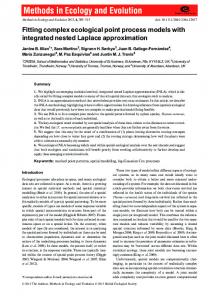
The analysis of forest fire occurrences is a research area that has been active for many years. Fire-history studies commenced in the early 20th century, mainly in the USA and Australia. Statistical modelling of forest fires appeared in the late 1970s with the works of Wilkins (1977) and Dayananda (1977) with fitting Poisson process to dataset. More recent statistical works include Pereira et al. (2013), Gabriel et al. (2017), and the references therein. Fire is the most important disturbance in a wide range of geographic scales (Figure 2.1) and it is difficult to visualize the existence of wide forest areas without the presence of an intense fire pattern. However, fire is considered a 19

20CHAPTER 2. SPATIO-TEMPORAL FOREST FIRE MODELLING WITH POINT PROCESSES

Figure 2.1: Worldwide counts of observed wildfire occurrence from 1996 to 2007 (Moritz et al., 2012). hazard to human life and property. Good management practices require understanding the role that biological and physical factors play in the pattern of fire occurrences in space and time, and to assess the potential risk posed by such fire pattern to human property, it is necessary to develop statistical models. In a forest stand, the risk of fire is usually related to variables such as air temperature and humidity, vegetation type, elevation and rainfall (Besie and Johnson, 1995). It is unlikely that proper conditions for fire ignition be present at the same time in a broad area; so, fire occurrence may be considered as a local phenomena. The local random nature of fire ignitions as well as its dynamics in time permit to idealize the occurrence of fires as a space–time point process. In recent decades, forest fires have become one of the main environmental problems and one of the most significant causes of forest destruction in Mediterranean countries. One such perspective comes from the statistical modelling of the space-time distribution of forest fires, while assessing which factors can be related to their existence. In fact in various locations around the globe, there are now many studies of the space-time patterns of forest fires risk. Without being exhaustive, and referring only to those more recent studies, we cite works on fires, above all, in Genton et al. (2006), Hering et al. (2009), Møller and Diaz-Avalos (2010), Juan et al. (2012), Pereira et al. (2013), Serra et al. (2014a), Serra et al. (2014b) and Gabriel et al. (2017). Table 2.1 is a summary of space-time point process models are used for forest fire occurences. In the following, we investigate them based on year of publication from nearest to farest in time. As we can see in Table 2.1, recently log-Gaussian Cox process is a favourite model in literature because it defines a class of flexible models that are particularly useful in the context of modelling aggregation relative to some underlying environmental field. These processes provide models for point patterns where the intensity function is supposed to come from a continuous Gaussian random

2.1. MODELLING APPROACH

21

Table 2.1: Summary of space-time point process models used for forest fires Authors Model Separability Estimation method Genton et Poisson process separable maximum pseudo al. (2006) likelihood Hering et al. Poisson process separable maximum pseudo (2009) likelihood Møller and Shot-noise Cox separable maximum Diaz-Avalos process likelihood (2010) Juan et Inhomogeneous separable maximum pseudo al.(2012) Area-Interaction likelihood process Pereira et al. Log-Gaussien Cox separable maximum (2013) process likelihood, INLA Serra et al. Log-Gaussien Cox separable INLA (2014a) process Serra et al. Poisson hurdle process separable INLA (2014b) Gabriel et Log-Gaussien Cox separable INLA al. (2017) process

field. In this sense, log Gaussian Cox processes are able to mix the two main areas of spatial statistics: point processes and geostatistics. The spatial dependence amongst locations depends on the spatial structure of the underlying random field depicting a nice and clear combination between the two areas of spatial statistics. Gabriel et al. (2017) analyzed daily records of fire events and burnt surfaces in Provence, France. First, they analyzed the dataset that allows to select relevant land use and climatic covariates. They then fitted a log-Gaussian Cox process including covariate information and nonparametric spatial and temporal effects. They showed that Log-Gaussian Cox processes can also deal with more complex structures, allowing further temporal inhibition at small spatial scales and thus providing more accurate predictions. They also studied inhibitive effects that arise locally in time and space after fire events with relatively large burnt surfaces. Serra et al. (2014a) analyzed the spatio-temporal patterns produced by those wildfire incidences by considering the influence of covariates on trends in the intensity of wildfire locations. They specified spatio-temporal log-Gaussian Cox process models. Their objective was twofold: (a) to evaluate which factors were associated with the presence of wildfires and their spatial distribution; and (b) to evaluate in time, the spatial variation of fire risk across Catalonia. They used two different kinds of log-linear models: Poisson regression and zero-inflated Poisson (ZIP) regression. The results of their analysis have provided statistical

Study area USA USA USA

Spain

Portugal Spain Spain France

22CHAPTER 2. SPATIO-TEMPORAL FOREST FIRE MODELLING WITH POINT PROCESSES evidence that areas closer to humans have more human induced wildfires, areas farther have more naturally occurring wildfires. Serra et al. (2014b) used a hurdle model to predict the occurrence of wildfires with point mass at zero followed by a truncated Poisson distribution for the nonzero observations. The hurdle Poisson model (Mullahy, 1986; King, 1989) is a modified count model with two processes, one generating the zeros and one generating the positive values. The two models are not constrained to be the same. The concept underlying the hurdle model is that a binomial probability model governs the binary outcome of whether a count variable has a zero or a positive value. If the value is positive, the “hurdle is crossed,” and the conditional distribution of the positive values is governed by a zero-truncated count model. The zero inflated Poisson model on the other hand is a mix of two models. One is a binomial process which generates structural zeros, and the second component a Poisson model with mean Λjt , which generates counts, some of which can be equal to zero. The zero inflated Poisson model then combines both components through a factor pi that represents the probability of the zero counts coming from the binomial component, and (1 − pi ) the probability that a zero comes from the Poisson component. Zero counts coming from the binomial component are also known as structural or excess zeros. Although the practical results are very similar in both approaches, zero inflated Poisson models are most appropriate in their case, since there are areas in which it is not possible for a wildfire to occur, either because they are urban, aquatic or do not have sufficient forest mass to make a wildfire possible. Pereira et al. (2013) modeled wildfires as coming from a Poisson distribution with a mean that varies according to some smooth spatial process. Actually, they fitted a spatio-temporal log-Gaussian Cox process and followed the stochastic partial differential equation (SPDE) approach. In study by Juan et al. (2012), research is conducted to provide analytical probabilistic models that mimic the reality of wildfires to assist land managers and foresters in Catalonia, Spain. Several different techniques are used and compared. First, a homogeneous Poisson process is used to analyze spatial clustering. The Poisson model used within this study builds confidence intervals based on a corresponding K-function from several simulations under the Poisson assumption of complete spatial randomness. Within the Poisson model, the second technique studied is an inhomogeneous Thomas model that analyzes each year and cause of ignition to better fit the clustering model. This model evaluates the joint effects of covariates (slope, aspect, hill shade and land use) as independent variables in linear regression model for intensity function. The final test of spatial patterns is seen in the use of the area-Interaction point process model (Baddeley and van Lieshout, 1995). This model is chosen because it is a more inclusive spatial model that displays inhomogeneity that considers covariate trends in an infinite number of interactions. All models are then fitted with a Papangelou function to find conditional intensity and create risk maps. Of all the techniques, the area-Interaction model is found to best fit the behavior of wildfire for most years and causes. Møller and Diaz-Avalos (2010) considered a spatio-temporal Cox point pro-

2.2. ESTIMATION APPROACH

23

cess models with a multiplicative structure for the driving random intensity, incorporating covariate information into temporal and spatial components, and with a residual term modelled by a shot-noise process. The model has strong flexibility and tractability through statistical analysis, using spatio-temporal versions of intensity and inhomogeneous K-functions, quick estimation procedures based on composite likelihoods and minimum contrast estimation, and easy simulation techniques. These advantages have been demonstrated based on a large data set consisting of more than 5000 wildfire accident locations. Shot noise Cox processes constitute a large class of Cox and Poisson cluster processes. Hering et al. (2009) reanalyzed wildfire data from the St. Johns River Water Management District in northeastern Florida with an inhomogeneous version of a homogenous K-function. They also used K-cross functions to study multitype point patterns, both under homogeneity and inhomogeneity assumptions. Finally, they described various point pattern models for the location of wildfires and investigate their adequacy by means of recent residual diagnostics. Genton et al. (2006) analyzed the spatio-temporal structure of wildfire ignitions in the St Johns River Water Management District in north-eastern Florida. They showed, using tools to analyse point patterns (e.g. the L-function), that wildfire events occur in clusters. Clustering of these events correlates with irregular distribution of fire ignitions, including lightning and human sources, and fuels on the landscape. They carried the analysis in three steps: purely temporal, purely spatial, and spatio-temporal. Their results showed that arson and lightning are the leading causes of wildfires in this region and that ignitions by railroad, lightning, and arson are spatially more clustered than ignitions by other accidental causes.

2.2

Estimation approach

A number of different approaches to parameter estimation have been used in the context of spatio-temporal point processes e.g. moment, likelihood and Bayesian-based methods. These are based on the same ideas as in classical statistics. Which estimation method is used for a specific data set depends on the model and the nature of the parameters and is to a certain extent also a matter of taste. As far as the performance of the estimators is concerned, these are usually required to be unbiased, and to have a small mean squared error (mse). Another requirement is that the estimators are consistent, i.e. that their increases with increasing window size. This is the case for many parameter estimators of stationary point processes if these are ergodic.

2.2.1

Classical methods

Classical methods of inference for spatio-temporal point processes are hampered by the intractability of the likelihood function for most models of interest. To

24CHAPTER 2. SPATIO-TEMPORAL FOREST FIRE MODELLING WITH POINT PROCESSES some extent, this difficulty has been alleviated by the development of Monte Carlo methods for calculating approximate likelihoods. Maximum likelihood methods are widely used in classical statistics, and many statisticians believe that they should also be preferred in point process statistics. Indeed, famous theorems by Fisher, Rao and Cram´er show that in classical statistics maximum likelihood estimators represent the ‘hard currency’ among the estimators as they are efficient, sufficient and consistent. Maximum likelihood method techniques can only be applied if the likelihood function – describing the probability of observing the data given the model – is known. This probability is maximised (with fixed data and variable parameters), yielding parameter estimators that best fit the data. However, often and particularly for stationary point processes, it is extremely difficult, even impossible, to find the likelihood function. As a result, the maximum likelihood method can only be applied to specific classes of models. These are Poisson processes and Cox processes. It is possible to apply the maximum likelihood method to spatio-temporal point patterns where the likelihood function is not known explicitly by approximating the likelihood function. This can be done in many ways e.g. pseudolikelihood method and Monte Carlo maximum likelihood. An interesting example of this approach is the pseudo-likelihood method. Consider in (1.27), intensity function depending on a parameter θ. If logarithm of intensity function is linear in θ, then the log-likelihood is concave, so there is a unique MLE. However, the MLE is not analytically tractable, so it must be computed using numerical algorithms such as Newton’s method. The method of maximum pseudo-likelihood was originally proposed by Besag (Besag, 1974) as a method for real-valued, spatially discrete processes. Besag et al. (1982) derived a point process version by considering a limit of binary-valued processes on a lattice, as the lattice spacing tends to zero. For a finite dimensional probability distribution, the pseudo-likelihood is the product of the full conditional distributions, i.e. the conditional distributions of each xi given the values of all other xj . Hence, if x is a set, i.e. x = (x1 , ..., xn ) and it has joint Q probability density f (x), n then the pseudo-likelihood is, in an obvious notation, i=1 f (xi |xj , j 6= i). For a point process, the pseudo-likelihood uses (Papangelou) conditional intensities in place of the full conditional distributions. As an alternative to traditional, parametric approaches, Møller and DiazAvalos (2010) suggest nonparametric methods such as kernel smoothing for analyzing spatial and temporal data on forest fires. Nonparametric techniques are particularly adaptive to anomalous behavior in the data and provide a new way of accessing a variety of different types of information about the way in which both intensity and magnitude of events evolve in time.

2.2.2

Bayesian methods

The Bayesian approach to statistical inference has recently become very popular, especially in the analysis of complex data sets. This is mainly a result of the development of Markov chain Monte Carlo methods, which has made it possible

2.2. ESTIMATION APPROACH

25

to apply Bayesian methods, since the early 1990s, to a much wider range of situations than had previously been possible. Not surprisingly, the Bayesian approach, together with MCMC methodology, has also made its way into point process theory. The Bayesian approach follows a different philosophy than the classical frequentist approach to statistical inference; the parameters and other unknown quantities, such as unobserved variates (covariates) and missing data, are considered random variables that are assumed to follow some probability distribution. As mentioned above, the unknown θ are further modelled with a prior distribution π(θ). The investigator’s uncertainty on θ given the data x is expressed by the posterior distribution π(θ|x). The posterior distribution is often difficult to handle and an analytical calculation of its characteristics is impossible in most cases due to the normalising integral in the denominator. However, MCMC methods can be applied to simulate from the posterior distribution. Recently, INLA (Integrated Nested Laplace Approximation) method (Rue et al., 2009) is used in the context of wildfires to perform the inference (see, e.g., Pereira et al. (2013), Serra et al. (2014a), Serra et al. (2014b) and Gabriel et al. (2017)). INLA is a method for Bayesian inference in structured additive regression models with a latent Gaussian field. INLA is an alternative to MCMC and combines analytical approximations with numerical integration, allowing to obtain the marginal posteriors for the latent fields and the marginal posteriors for the hyper-parameters in relatively short computational time and in general, which makes it possible to perform Bayesian analysis in an automatic, streamlined way, and to compute model comparison criteria and various predictive measures so that models can be compared and the model under study can be challenged. The fundamental idea of INLA consists in applying the device of Laplace approximation to integrate out high-dimensional latent components. This theoretical foundation is combined with efficient algorithms and numerical tricks and approximations to ensure a fast yet accurate approximation of posterior marginal densities of interest like those of the predictors or of hyperparameters. According to Table 2.1, Pereira et al. (2013), Serra et al. (2014a), Serra et al. (2014b) and Gabriel et al. (2017) used INLA approach for estimation. Pereira et al. (2013) also used maximum likelihood method. Møller and DiazAvalos (2010) used maximum likelihood method. Hering et al. (2009), Genton et al. (2006) and Juan et al.(2012) used maximum pseudo-likelihood method. Conclusion and discussion As we see in Table 2.1 (study area), recently the modelling forest fire occurences in Mediterranean region be an interesting challenge. Fire risk is highly important in the Mediterranean region because of its seasonal nature, with summers of high temperatures and low humidity. On the other hand, as we see in Table 2.1, the models are assumpted separable (see Section 1.2) while using of non-separable covariance structure for space and time is clearly suggested by the preliminary data analysis reported in Section 3 of Pereira et al. (2013) or

26CHAPTER 2. SPATIO-TEMPORAL FOREST FIRE MODELLING WITH POINT PROCESSES Fuentes-Santos et al. (2018) suggested, according to their results, it should be used a nonseparable shot-noise Cox process model in Møller and Diaz-Avalos (2010) and the spatio-temporal structure of the distribution of forest fires is very complex because, in practice, the dependence can’t be separated in space and time. If the spatial heterogeneity of forest fires will depend on the spatial distribution of current land use (vegetation, urban zones, wetlands), it also depends on the past, because changes in vegetation due to fires will affect the probability of fire occurrence during the regeneration period. As a future work, we will consider some new spatio-temporal point processes in non-separable framework with multi-scale structures for modeling the forest fire occurences in the PACA region based on the Prom´eth´ee database. Hence, according to the above discussion, we investigate the non-separable spatio-temporal models in geostatistics and point process theory in Chapter 3 and multi-scale structures point processes in Chapter 4.

Chapter 3

Space time non-separable point process models When it comes to statistical analysis of space-time point processes, separability is a popular assumption. The obvious reason is the simplification of the inference: if the process (or at least its first- or second-order propeties) is separable the inference about the quite complicated space-time model can be based on the properties of the lower dimensional and easier to handle spatial and temporal marginal processes. For a separable process, the spatial and temporal structures can be modeled separately. Therefore, many techniques that have been developed and successfully implemented in time series analysis and spatial point processes and geostatistics can be used with this subclass of separable spatial temporal processes. Another advantage of assuming separability is the computational efficiency. On the other hand, separability is a restriction that will often fail to model the time dynamics of the process realistically. One reason for the widespread use of separable models is the lack of non-separable models in the literature and the complexity of the statistical inference. Separability is a convenient working assumption, but may be too inflexible for some applications. For example, Fuentes-Santos et al. (2018) detected departure from separability in all the wildfire patterns under study or Pereira et al. (2013) suggested to use of non-separable covariance structure for space and time by the preliminary data analysis. As mentioned in Chapter 1, first-order and second-order separability factor into purely temporal and purely spatial components in first-order propeties (intensity function) and second-order propeties (K-function and pair correlation function). In this Chapter, first we investigate the first-order and second-order separability. Then, we investigate the classes of non-separable models in random field models and testing separability in spatio-temporal point processes. We emphasize that the space component is in Rd and we will show it with a bold letter. 27

28CHAPTER 3. SPACE TIME NON-SEPARABLE POINT PROCESS MODELS

3.1

First-order separability

We can extend (1.1) to spatio-temporal point prcess as following. Considering the intensity measure Λ(A × B) = E[N (A × B)], A × B ⊆ W × T , we have that Z Z Λ(A × B) = λ(x, t)dxdt, (3.1) A

B

and we refer to λ(x, t) as the intensity function of X. It is often convenient to make the pragmatic assumption that first-order effects are separable, i.e. that (almost everywhere) the intensity function can be written λ(x, t) = ρ(x)µ(t), (3.2) hereby Z Λ(A × B) = E(N (A × B)) =

Z ρ(x)dx

A

µ(t)dt,

(3.3)

B

where ρ(.) and µ(.) are non-negative functions. Note that these functions are not unique. This is referred to as first-order spatio-temporal separability. Here any effects that are non-separable are interpreted as second-order effects, rather than first-order effects. A stationary spatio-temporal point process X is automatically first-order separable since its intensity λ = λ1 λ2 ≥ 0 is constant. If X is space-stationary, it is also first-order separable with λ1 being a non-negative constant. Similarly, when X is time-stationary, first-order separability holds with λ2 being a nonnegative constant. When X is a finite spatio-temporal point process or taken as the restriction of a spatio-temporal point process to W × T , it may be natural, at times, to project X onto W and T , and thus deal with the space and time components of X separately. Following Møller and Ghorbani (2012), let Xspace = {x : (x, t) ∈ X, t ∈ T }, Xtime = {t : (x, t) ∈ X, x ∈ W }.

(3.4)

When we have obtained Xspace and Xtime , we may also define the marginal spatial and temporal intensity functions λspace and λtime , respectively, as Z Z λspace (x) = ρ(x) µ(t)dt and λtime (t) = µ(t) ρ(x)dx, (3.5) T

W

whereby λ(x, t) ∝ λspace (x)λtime (t), with λ, λspace , λtime all being constant when X is homogeneous. When estimating the intensity function we are challenged with the task of ˆ : W × T → R+ . Suppose we have obtained estimates finding an estimate λ ˆ space (.) and λ ˆ time (.) (e.g. see Appendix of Møller and Ghorbani, 2012; of λ Ghorbani, 2013). Since λspace and λtime are unbiased estimates of the expected R R ˆ space (x)dx = ˆ number of observed points, i.e. W λ λ (t)dt = n, then the T time estimate of the spatio-temporal intensity function given by ˆ space (x)λ ˆ time (t). ˆ t) = 1 λ λ(x, n

(3.6)

3.2. SECOND-ORDER SEPARABILITY

29

also becomes an unbiased estimate of the expected number of observed points, i.e. Z Z ˆ t)dxdt = n. λ(x, (3.7) W

T

For non-parametric estimation of the spatial intensity function, it is common in using a kernel estimate, ˆ space (x) = λ

n X κ (x − xi )

cW (xi )

i=1

where κ (x) =

, x ∈ W.

1 x κ( ), 2 

(3.8)

(3.9)

and κ(.) is a bivariate kernel and  > 0 is a smoothing parameter, where Z cW (xi ) = κ (x − xi )dx, (3.10) W

is R an edge-correction factor included in the estimation to guarantee that ˆ λ (x)dx = n. Similarly, we may also estimate λtime (t) nonW space parametrically by means of kernel estimators. Although these non-parametric estimators may only lead to approximately unbiased estimates, we will still employ equation (3.6) for the estimation of λ(x, t).

3.2

Second-order separability

Similarly to the case of first-order separability, at times one makes the assumption that the second-order spatio-temporal effects are separable. Specifically, the pair correlation function is said to be separable if g((x, s), (y, t)) = g1 (x, y)g2 (s, t)

(3.11)

where g1 and g2 are non-negative functions. Under assumption of second-order intensity-reweighted stationarity, it can be rewritten as g(u, v) = g1 (u)g2 (v),

(3.12)

moreover, separability of K-function into purely spatial and temporal components is defined K(u, v) = K1 (u)K2 (v), where the spatio-temporal inhomogeneous K-function is defined Z Z v K(u, v) = g(x, t)dxdt. (3.13) ||x||≤u

−v

We can also define spatial and temporal components for pair correlation function similar to intensiy function. We assume that X has intensity function

30CHAPTER 3. SPACE TIME NON-SEPARABLE POINT PROCESS MODELS λ and pair correlation function g (see Møller and Waagepetersen (2004)). Then Z Z f ((x, s), (y, t))g((x, s), (y, t))d(x, s)d(y, t) = E

6= X (x,s),(y,t)∈X

f ((x, s), (y, t)) λ(x, s)λ(y, t)

(3.14) for any non-negative Borel function f defined on (Rd × R) × (Rd × R). Where P6= means that (x, s) 6= (y, t) and let a/0 = 0 for a ≥ 0. Hence, The pair correlation function gspace of the spatial component process Xspace satisfies Z Z f (x, y)gspace (x, y)dxdy = E

6= X x,y∈X

f (x, y) λspace (x)λspace (y)

(3.15)

for any non-negative Borel function f defined on Rd × Rd . Similarly, gtime can be defined. The corresponding K-functions are Z Kspace (u) = gspace (x)dx, u > 0, (3.16) ||x||≤u

and

Z Ktime (v) =

gtime (t)dt, v > 0.

(3.17)

|t|≤v

ˆ space and K ˆ time are found in Møller and Ghorbani (2012). The estimators K As mentioned, the separability in second order is the separability of two functions (K-function or pair correlation function). In the case where the point processes models depend on an underlying random fields (for example Cox processes) the second-order propeties are linked to the covariance of the random fields. Hence, the second-order separability is due to the separability of the covariance. A useful summary statistic of space-time process X(x, t) in a random field framework is its covariance function γ(u, v) = cov(X(x, t), X(x − u, t − v)).

(3.18)

The definition of (weak) stationarity is that the covariance depends only on the separation (u, v) and not on the location (x, t). The covariance function is particularly informative for Gaussian fields, as Gaussian fields are completely characterized by their mean and covariance function. Since the spatio-temporal covariance function itself summarizes many aspects of the process, spatio-temporal studies often propose a series of simplifying assumptions about the process in question in order to estimate the spatiotemporal covariance function in the simplest possible way. The most important among them is the separability assumption, meaning γ(u, v) = γ1 (u)γ2 (v).

(3.19)

3.2. SECOND-ORDER SEPARABILITY

31

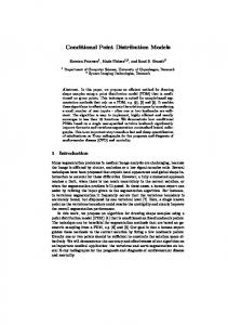
Figure 3.1: Schematic illustration of the relationships between separable, fully symmetric, stationary, and compactly supported covariances within the general class of (stationary or non-stationary) space-time covariance functions. An analogous scheme applies to correlation structures. Many statistical tests for separability have been proposed recently and are based on parametric models, likelihood ratio tests and subsampling, or spectral methods. A related notion is that of full symmetry (Gneiting, 2002; Stein, 2005). The space-time process X has fully symmetric covariance if γ(u, v) = γ(−u, v) = γ(u, −v) = γ(−u, −v),

(3.20)

for all (u, v) ∈ Rd × R. Separability forms are a special case of full symmetry. Hence, covariance structures that are not fully symmetric are nonseparable, and tests for full symmetry can be used to reject separability. Figure 3.1 summarizes the relationships between the various notions in terms of classes of space-time covariance functions, and an analogous scheme applies to correlation structures. The largest class is that of general, stationary or non-stationary covariance functions. A separable covariance can be stationary or non-stationary, and similarly for fully symmetric covariances. However, a separable covariance function is always fully symmetric, but not vice versa, and this has implications in testing and model fitting. In particular, to reject separability it suffices to reject full symmetry. Note that in general, second-order separability is implied by, but does not imply, independence of the spatial and temporal component processes. However, a Poisson process has independent components if and only if it is first-order separable.

32CHAPTER 3. SPACE TIME NON-SEPARABLE POINT PROCESS MODELS

3.3

Non-separability in random field models

Although separability is a convenient assumption, it is unrealistic in many applications, hence this strong limitation has led several authors to propose nonseparable classes of covariance models. In this section, some well-known nonseparable stationary covariance models have been investigated. Different forms of non-separability for space–time covariance functions have been recently defined in the literature. The first attempt at an analysis of nonseparability was that of Cressie and Huang (1999). They introduced classes of nonseparable stationary covariance functions to model space-time interactions. They based their approach on Fourier transforms, and used Bochner’s Theorem (1955) whereby a continuous function is defined as positive definite if and only if, it is the Fourier transform of a finite nonnegative measure. Another important contribution to the analysis of nonseparable spatio-temporal models was made by Gneiting (2002) who proposed a general class of nonseparable, stationary covariance functions for spatio-temporal random fields directly in the space-time domain (a construction not based on the inversion of a Fourier transformation). Since covariance models have different features, a comparative study among some of them is useful to underline the importance of choosing a suitable model by taking into account the characteristic behaviour of the models. De Iaco (2010) proposed a comparative study among some classes of space–time covariance functions as following.

3.3.1

Bochner’s Theorem

The celebrated theorem of Bochner (1955) states that a continuous function is positive definite if and only if it is the Fourier transform of a finite nonnegative measure. This allows for the following characterization of stationary space- time covariance functions. Theorem 3.3.1. (Bochner) Suppose that γ is a continuous and symmetric function on Rd × R. Then γ is a covariance function if and only if it is of the form Z Z > γ(u, v) = ei(u ω+vτ ) dF (ω, τ ), (u, v) ∈ Rd × R, (3.21) where F is a finite, non-negative and symmetric measure on Rd × R. In other words, the class of stationary space-time covariance functions on Rd × R is identical to the class of the Fourier transforms of finite, non-negative and symmetric measures on this domain. The measure F in the representation (3.21) is often called the spectral measure. If γ is integrable, the spectral measure is absolutely continuous with Lebesgue density Z Z > −(d+1) f (ω, τ ) = (2π) e−i(u ω+vτ ) γ(u, v)dudv, (ω, τ ) ∈ Rd × R, (3.22)

3.3. NON-SEPARABILITY IN RANDOM FIELD MODELS

33

and f is called the spectral density. If the spectral density exists, the representation (3.21) in Bochner’s theorem reduces to Z Z > γ(u, v) = ei(u ω+vτ ) f (ω, τ )dωdτ, (u, v) ∈ Rd × R, (3.23) and γ and f can be obtained from each other via the Fourier transform. In terms of the joint process, separability can be formulated as γ(u, v) =

γ(u, 0)γ(0, v) , γ(0, 0)

(3.24)

for all (u, v) ∈ Rd × R, where γ(u, 0), γ(0, v) and γ(0, 0) are the purely spatial covariance function, the purely temporal covariance function and the variance of the process. For fully symmetric covariances, Bochner’s theorem can be specialized as follows. Theorem 3.3.2. Suppose that γ is a continuous on Rd × R. Then γ is a stationary, fully symmetric covariance if and only if it is of the form Z Z γ(u, v) = cos(u> ω)cos(vτ )dF (ω, τ ), (u, v) ∈ Rd × R, (3.25) where F is a finite, non-negative measure on Rd × R.

3.3.2

Cressie-Huang representation

The following result of Cressie and Huang (1999) characterizes the class of stationary space-time covariance functions under the additional assumption of integrability. Theorem 3.3.3. (Cressie and Huang) Suppose that γ is a continuous, bounded, integrable, and symmetric function on Rd × R. Then γ is a stationary covariance if and only if Z > ρ(ω, v) = e−iu ω γ(u, v)du, v ∈ R, (3.26) is positive definite for almost all ω ∈ Rd . Cressie and Huang (1999) used Theorem 3.3.3 to construct stationary spacetime covariance functions through closed form Fourier inversion in Rd . Specifically, they considered functions of the form Z > γ(u, v) = eiu ω ρ(ω, v)dω, (u, v) ∈ Rd × R, (3.27) where ρ(ω, v), v ∈ R, is a continuous positive definite function for all ω ∈ Rd . Gneiting (2002) gave a criterion that is based on this construction but does

34CHAPTER 3. SPACE TIME NON-SEPARABLE POINT PROCESS MODELS not depend on closed form Fourier inversion and does not require integrability. Recall that a continuous function ϕ(r) defined for r > 0 or r ≥ 0 is completely monotone if it possesses derivatives ϕ(n) of all orders and (−1)n ϕ(n) (r) ≥ 0 for r > 0 and n = 0, 1, 2, .... Theorem 3.3.4. (Gneiting) Suppose that ϕ(r), r ≥ 0, is a completely monotone function, and that ψ(r), r ≥ 0, is a positive function with a completely monotone derivative. Then γ(u, v) =

1 ψ(v 2 )d/2

ϕ(

||u||2 ), ψ(v 2 )

(u, v) ∈ Rd × R,

(3.28)

is a stationary covariance function on Rd × R. All valid examples given by Cressie and Huang(1999) are special cases of the model proposed by Gneiting (2002). The specific choices ϕ(r) = σ 2 exp(−crδ ) and ψ(r) = (1 + arα )β recover Equation (14) of Gneiting (2002) and yield the parametric family γ(u, v) =

σ2 c||u||2δ ), exp(− (1 + a|v|2α )βδ (1 + a|v|2α )βd/2

(u, v) ∈ Rd × R,

(3.29)

of stationary space-time covariance functions. Here, a and c are nonnegative scale parameters of time and space, respectively. The smoothness parameters α and δ and the space-time interaction parameter β take values in (0, 1], and σ 2 is the variance of the spatio-temporal process. The purely spatial covariance function is of the powered exponential form, and the purely temporal covariance function belongs to the Cauchy class. Clearly, any stationary covariance of the form (3.28) is fully symmetric. Furthermore, under the assumption of full symmetry the test functions ρ(ω, v) of Theorem 3.3.3 are real-valued and symmetric functions of v ∈ R. If γ is not fully symmetric then ρ(ω, v) is generally complex-valued. For instance, the function γ(u, v) = exp(−u2 + uv − v 2 ) has Fourier transform proportional to exp(− 31 (ω 2 + ωτ + τ 2 )) and therefore is a stationary covariance on R × R. The associated test function ρ(ω, v), v ∈ R, is proportional to exp(− 14 (3v 2 + 2iωv)) and positive definite yet generally complex-valued.

3.3.3

Fully symmetric, stationary covariance functions

Non-separable, fully symmetric stationary space-time covariance functions can be constructed as mixtures of separable covariances. In view of Theorem 3.3.2, the construction is completely general. Theorem 3.3.5. Let µ be a finite, nonnegative measure on a non-empty set Θ. Suppose that for each θ ∈ Θ, γ1θ and γ2θ are stationary purely spatial and purely temporal covariances on Rd and R, respectively, and suppose that γ1θ (0)γ2θ (0) has finite integral over Θ. Then Z γ(u, v) = γ1θ (u)γ2θ (v)dµ(θ), (u, v) ∈ Rd × R, (3.30)

3.3. NON-SEPARABILITY IN RANDOM FIELD MODELS

35

is a stationary covariance function on Rd × R. Explicit constructions of the form (3.30) have been reported by various authors. Perhaps the simplest special case is the product-sum model of De Iaco et al. (2001), γ(u, v) = k1 γ11 (u)γ21 (v) + k2 γ12 (u) + k3 γ23 (v)

(3.31)

where k1 , k2 and k3 are nonnegative coefficients and γ11 , γ12 and γ21 , γ23 are stationary, purely spatial and purely temporal covariance functions, respectively.

3.3.4

Positive and negative non-separability

We need a criterion for facilitating to choose a more suitable class of covariance models for the spatio-temporal data. Rodrigues and Diggle (2010) classified the nonseparable stationary covariance models to positive and negative nonseparability as follows. Let γ(u, v) be a spatial–temporal stationary covariance function and ρ(u, v) the corresponding spatial–temporal correlation function and define r(u, v) =

ρ(u, v) , ρ(u, 0)ρ(0, v)

(3.32)

where ρ(u, v) > 0, ρ(u, 0) > 0 and ρ(0, v) > 0. Then, a covariance function γ is positively non-separable at (u, v) if r(u, v) > 1, and negatively non-separable at (u, v) if r(u, v) < 1. The models with ρ(u, v) < 0 is not considered, although mathematically possible, because it is uncommon in practice. All valid examples given by Cressie and Huang (1999) have positive nonseparability; those which would correspond to negative non-separability have been shown by Gneiting (2002) to be invalid. The following result shows that (3.30) cannot accommodate negative nonseparability. Theorem 3.3.6. The class of covariance functions (3.30) cannot accommodate negative nonseparability. Proof. See Rodrigues and Diggle (2010). As an another result, the following result shows that class of product–sum covariance models proposed by De Cesare et al. (2001) cannot produce positive non-separable covariance functions. Theorem 3.3.7. The class of product–sum covariance models γ(u, v) = k1 γ1 (u)γ2 (v)+k2 γ1 (u)+k3 γ2 (v), where k1 > 0, k2 ≥ 0 and k3 ≥ 0 are constants, cannot accommodate positive non-separability. Proof. See Rodrigues and Diggle (2010).

36CHAPTER 3. SPACE TIME NON-SEPARABLE POINT PROCESS MODELS Rodrigues and Diggle (2010) also proposed a simple class of non-separable covariance functions, which accommodates negative, zero and positive nonseparability. Consider covariance function γ(u, v) =

γ(0, 0) 1 (ρ1 (u)ρ12 (v) + ρ21 (u)ρ22 (v)), 2

(3.33)

where ρ11 (u), ρ21 (u), ρ12 (v), ρ22 (v) are, respectively, two non-negative, valid and integrable spatial and two non-negative, valid and integrable temporal correlation functions. Note that if either ρ11 (u) = ρ21 (u) or ρ12 (v) = ρ22 (v) then (3.33) gives a separable model. Let d(u, v) = γ(u, v)γ(0, 0) − γ(u, 0)γ(0, v). It follows that γ(u, v) =

γ(0, 0)2 1 (ρ1 (u) − ρ21 (u))(ρ12 (v) − ρ22 (v)). 4

(3.34)

If ρ12 (v) > ρ22 (v) for all v > 0, then γ(u, v) is positively or negatively nonseparable at (u, v) when ρ11 (u) is greater or smaller than ρ21 (u), respectively. In Rodrigues and Diggle (2010), the separability condition in (3.32) and the two types of non-separability (positive and negative) are given for a fixed (u, v) and without pointing out that a covariance function usually depends on a vector of parameters Θ. Hence, a generalization of the above pointwise definition of non-separability proposed by De Iaco and Posa (2013). De Iaco and Posa (2013) defined the uniformly positive and negative nonseparable covariance model as follows. Let γ(u, v; Θ) be a spatial–temporal stationary covariance function and ρ(u, v; Θ) the corresponding spatial–temporal correlation function, where Θ is a vector of parameters. Let r(u, v; Θ) =

ρ(u, v; Θ) , ρ(u, 0; Θ)ρ(0, v; Θ)

(3.35)

where ρ(u, v; Θ) > 0, ρ(u, 0; Θ) > 0 and ρ(0, v; Θ) > 0. Then, the covariance function γ is uniformly positive non-separable, if r(u, v; Θ) > 1 ∀(u, v) ∈ Rd × R, ∀Θ,

(3.36)

or alternatively it is uniformly negative non-separable, if r(u, v; Θ) < 1 ∀(u, v) ∈ Rd × R, ∀Θ.

(3.37)

On the other hand, if r(u, v; Θ) > 1 for some (u, v; Θ), the covariance function is pointwise positive non-separable at the same (u, v; Θ); alternatively, it is pointwise negative non-separable at (u, v; Θ), if r(u, v; Θ) < 1 for the corresponding (u, v; Θ). Analogously, the non-separability index can be expressed in terms of the difference d(u, v; Θ) between ρ(u, v; Θ) and ρ(u, 0; Θ)ρ(0, v; Θ), that is d(u, v; Θ) = ρ(u, v; Θ) − ρ(u, 0; Θ)ρ(0, v; Θ),

(3.38)

3.3. NON-SEPARABILITY IN RANDOM FIELD MODELS

37

or equivalently d0 (u, v; Θ) = γ(u, v; Θ)γ(0, 0; Θ) − γ(u, 0; Θ)γ(0, v; Θ).

(3.39)

The sign of (3.38) and (3.39) will give information about the kind of nonseparability. Then, a covariance function which is uniformly positive (negative) non-separable, is also pointwise positively (negatively) non-separable, but the converse is not true. Thus, the index of non-separability depends on the specific lag and on the model parameters. According to the above definition, De Iaco and Posa (2013) showed some classes of non-separable stationary space–time covariance models are uniformly positive (negative) non-separable; on the other hand, there exist stationary space–time covariance models which are positively non-separable for a particular choice of (u, v), or the vector of parameters Θ, and negatively non-separable for a different choice of (u, v), or the vector of parameters Θ. As mentioned above, recently, the type of non-separability of two wide classes of space–time covariance models, such as the Gneiting class of space–time covariance models (Gneiting, 2002) and the product–sum covariance models (De Cesare et al., 2001; De Iaco et al., 2001), was analyzed by Rodrigues and Diggle (2010). Gneiting class of space-time covariance models for d = 2 is defined as follows: γ(u, v; Θ) =

||u||2 σ2 ϕ( ; θ2 ), ψ(v 2 ; θ1 ) ψ(v 2 ; θ1 )

(3.40)

where Θ = (θ1 , θ2 ) is the parameter vector, ϕ(v; θ2 ), v ≥ 0, is a completely monotone function and ψ(v; θ1 ), v ≥ 0, is a positive valued function with completely monotone derivative, ϕ(0; θ2 ) = 1 and ψ(0; θ1 ) = 1. The spatial–temporal covariance function defined as in (3.40) is characterized by a uniformly positive non-separability, unless ϕ be constant. According to above definition, the class of product–sum covariance models γ(u, v; Θ) = k1 γ1 (u; θ1 )γ2 (v; θ2 ) + k2 γ1 (u; θ1 ) + k3 γ2 (v; θ2 ),

(3.41)

where Θ = (θ1 , θ2 , k, k2 , k3 ), k1 > 0, k2 ≥ 0, k3 ≥ 0, γ1 and γ2 are temporal and spatial covariance models, with k2 , k3 6= 0 and 0 < γ1 (u; θ1 ) < γ1 (0; θ1 ), 0 < γ2 (v; θ2 ) < γ2 (0; θ2 ) when (u, v) 6= (0, 0), is characterized by a uniformly negative non-separability. Note that Rodrigues and Diggle (2010) simply defined the classes of models (3.40) and (3.41) positive and negative nonseparable, respectively. Similarly, the linear models, obtained from (3.41) when k1 = 0, are uniformly negative non-separable, since the sign of the difference d, associated with the product–sum (3.41), does not depend on the coefficient k1 .

38CHAPTER 3. SPACE TIME NON-SEPARABLE POINT PROCESS MODELS

3.4

Link between geostatistics and point process models

In this section, we try to show methods for distinguishing if a point process can be considered a special class of a random field and then geostatistical methods proposed in last section suffice to interpret results. According to Section 4.4 of Diggle and Ribeiro (2007), we present two quite different ways for links and conexions between both models as follows. Cox processes In geostatistics, we wish to make inferences about a spatially and temporaly continuous phenomenon, S = {S(x, t) : (x, t) ∈ Rd × R}, which is not directly observable. Instead, we observe discrete data, Y, which is stochastically related to S. By formulating a stochastic model for S and Y jointly and applying Bayes Theorem we can, in principle, derive the conditional distribution of S given Y, and so use the observed data, Y, to make inferences about the unobserved phenomenon of scientific interest, S. In geostatistical models, we abled to represent Y as a vector Y = (Y1 , ..., Yn ) in which each Yi is associated with a location xi and time ti , the Yi are conditionally independent given S, and the conditional distribution of Yi given S only depends on S(xi , ti ). As we mentined, a Cox process is a point process in which there is an unobserved, non-negative-valued stochastic process S = {S(x, t) : (x, t) ∈ Rd × R} such that, conditional on S, the observed point process is an inhomogeneous Poisson process with spatially and temoraly varying intensity S(x, t). Models of this kind fit into the general geostatistical framework whereby the model specifies the distributions of an unobserved process S and of an observed set of data Y conditional on S, except that now the conditional distribution of Y given S is that of a Poisson process generating a random set of points (xi , ti ) ∈ Rd × R, rather than of a finite set of measurements Yi at pre-specified locations (xi , ti ). The analogy is strengthened by the fact that the conditional Poisson process of Y given S is the point process analogue of mutually independent Yi given S when each Yi is a measured variable. One of the more tractable forms of Cox process is the log-Gaussian Cox process, in which log S is a Gaussian process. Assume that S(., .) is stationary, and denote by µ and γ(., .) its mean and covariance function. Then, the mean and covariance function of the intensity surface, Λ(x, t) = exp{S(x, t)}, are λ = exp{µ+0.5γ(0, 0)}, which also represents the expected number of points per unit area in the Cox process, and φ(x, t) = λ2 (exp{γ(x, t)} − 1) (It follows from the moment properties of the log Normal distribution). For the log-Gaussian Cox process the function K(u, v) by (1.20) takes the form Z vZ u K(u, v) = πu2 v + 2πλ−2 φ(x, t)xdxdt, (3.42) 0

0

and we have by (1.21) g(u, v) = exp{γ(u, v)}.

(3.43)

3.4. LINK BETWEEN GEOSTATISTICS AND POINT PROCESS MODELS39 Log Gaussian Cox point processes define a class of flexible models that are particularly useful in the context of modelling aggregation relative to some underlying unobserved environmental field (Illian et al., 2008; Simpson et al., 2011). These processes provide models for point patterns where the intensity function is supposed to come from a continuous Gaussian random field. In this sense, log Gaussian Cox point processes are able to mix the two main areas of spatial statistics, point processes and geostatistics. The spatial dependence amongst locations depends on the spatial structure of the underlying random field depicting a nice and clear combination between the two areas of spatial statistics. By this way, point process models are connected to geostatistics with replacing the mesurement process by a point process.

Preferential sampling A typical geostatistical data-set consists of a finite number of locations and time (xi , ti ) and associated measurements Yi . If, in this setting, we acknowledge that both the measurements and the locations are stochastic in nature, then a model for the data is a joint distribution for measurements and locations and time, which we represent formally as [X, Y ]. We usually assume that sampling is nonpreferential i.e., sampling and measurement processes are independent and the joint distribution of X and Y factorises as [X, Y ] = [X][Y ]. If, in contrast, sampling is preferential, then one of two possible factorisations of the joint distribution of X and Y is as [X, Y ] = [X][Y |X]. Hence, the implicit inferential target of a conventional geostatistical analysis, which analyses only the data Y , is the conditional distribution [Y |X], whereas the intended target is usually the unconditional distribution [Y ], and there is no reason in general to suppose that the two are equal (see Diggle and Ribeiro (2007) for more details). Models for preferential sampling can also be considered as models for marked point processes. Marks may be qualitative or quantitative. In this context, it is not necessary for the mark to exist at every point in space, only at each point of the process, for example the points could be the locations of individual trees in a forest and the marks might denote the species (qualitative) or height (quantitative) of each tree. However, the marks could also be the values, at each point, of an underlying spatially continuous random field. In this case, the model in which the mark process is independent of the point process is called the random field model. The random field model for a marked point process is therefore the counterpart of non-preferential sampling for a geostatistical model. By this way, actually, in some applications the set of locations at which measurements are made should strictly be treated as a point process. This second aspect is usually ignored by making the analysis of the data conditional on the observed locations, although the conditioning is seldom made explicit.

40CHAPTER 3. SPACE TIME NON-SEPARABLE POINT PROCESS MODELS

3.5

Non-separability in point process models

For a nonseparable spatio-temporal point process, the spatio-temporal point patterns may not be analysed by a separate spatial point pattern analysis and a time series analysis. This because the distributions of the spatial point patterns are then different for different times. There exists few literature that assume the non-separability in point processes. On the other hand, the hypothesis of separability in space and time is often assumed without any test in the literature because it allows to decompose the problem in two modeling steps, one in space and one in time, or to consider separable covariance matrices. Separability is a convenient property, but there is little written about how to formally test for it. There are a few tests for certain kinds of models, spatial-temporal marked point processes (Schoenberg, 2004; Chang and Schoenberg, 2011; Assuncao and Maia, 2007; Diaz-Avalos et al., 2013), spatio-temporal point processes (Møller and Ghorbani, 2012; Fuentes-Santos et al., 2018) and testing the separability has been tested by nonparametric tests calibrated through simulations of separable point processes by them. An excellent discussion of a diagnostic procedure for checking the hypothesis of second-order spatio-temporal separability can be found in Møller and Ghorbani (2012) as follows. Intuitively, Equations (3.2), (3.12) and (3.14) imply that the probability of observing a pair of points from X occurring jointly in each of two infinitesimally small sets with centers (x, s), (y, t) and volumes dxds, dydt is (ρ(x)ρ(y)g1 (x − y)dxdy)(µ(s)µ(t)g2 (s − t)dsdt) (3.44) which is a product of a function of the locations (x, y) and the areas (dx, dy) and a function depending on the times (s, t) and the lengths (ds, dt) and we have gspace (x) = cspace g1 (x), gtime (t) = ctime g2 (t), (3.45) where cspace and ctime are constants (see equations (15) and (16) of Møller and Ghorbani, 2012). Hence, by Equations (3.12), (3.13), (3.16), (3.17) and (3.45), spatio-temporal separability of g implies that the function D(u, v) =

K(u, v) Kspace (u)Ktime (v)

(3.46)

is constant and equal to 1/(cspace ctime ). Note that in the Poisson case, g = 1 ˆ and hence D = 1. Under the hypothesis of spatio-temporal separability of g, D should be expected to be approximately equal to 1/(cspace ctime ). Fuentes-Santos et al. (2018), based on this belief that testing whether the intensity function of a spatio-temporal point process is separable should be one of the first steps in the analysis of any observed pattern, proposed a new nonparametric test for first-order separability. They estimated the ratio between the spatiotemporal intensity function and the first-order intensity of the spatial point process and checked whether it depends on the spatial locations through a no-effect test as following.

3.5. NON-SEPARABILITY IN POINT PROCESS MODELS

41

Let λ0 (x, t) = λ(x, t)/n and ρ0 (x) = ρ(x)/n be the densities of event locations of S = {(xi , ti ), i = 1, ..., N )} ⊂ W × TR ⊂R R2 × R and X = R {xi , i = 1, ..., N } ⊂ W ⊂ R2 , respectively, where n = T W λ(x, t)dxdt = W ρ(x)dx is the expected number R of events of both the spatial and spatiotemporal point processes and ρ(x) = T λ(x, t)dt. The ratio r(x, t) =

λ0 (x, t) λ(x, t) = ρ(x) ρ0 (x)

(3.47)

can be seen as a spatiotemporal relative risk function. The kernel estimator of the spatiotemporal density of event locations is ˆ 0,H ,h (x, t) = λ s t

PN

i=0

−1/2

κs (Hs (x − xi ))κt (h−1 t (t − ti )) 1(N >0) N |H|1/2 ht pHs ,ht (x, t)

(3.48)

where the kernel functions, κs (.) and κt (.), are assumed to be symmetric. Hs is the two-dimensional bandwidth matrix for the spatial component and ht R R is the bandwidth forRthe temporal component. p (x, t) = κ H ,h s,H s t s (x − T W R u)κt,ht (t−v)dudv = W κs,Hs (x−u)du = κ (t−v)dv is the spatiotemporal t,h t T R R edge corrector, where pHs (x) = W κs,Hs (x − u)du and pht (t) = T κt,ht (t − v)dv represent, respectively, the bivariate edge corrector for the spatial locations and the univariate edge corrector for the temporal component. The kernel estimator of the spatial density function is PN ρˆ0,H (x) =

κs (H −1/2 (x − xi )) 1(N >0) N |H|1/2 pH (x)

i=0

(3.49)

where κs (.) is the same bivariate kernel used in the spatial component of R ˆ 0,H ,h (x, t), H is a bivariate bandwidth matrix, and pH (x) = λ κ (x−u)du s t W s,H is the edge-correction term. Hence, by applying kernel smoothing to estimate the log-ratio function l(x, t) = log(λ0 (x, t)/ρ0 (x)), estimator for the log-ratio function is ˆ ˆl(x, t) = log λ0,Hs ,ht (x, t) . (3.50) ρˆ0,H (x) For a separable spatio-temporal point process, λ(x, t) = ρ(x)µ(t); therefore, the log-ratio function, l(x, t) = log(λ(x, t)/ρ(x)), does not depend on the spatial locations, x, for any t ∈ T . This suggests using a regression test that checks whether the log-ratio function, l(x, t), depends on the spatial locations of events as a basis for a separability test (see Fuentes-Santos et al. (2018) for more details in simulation studies, comparison with former methods and application in real dataset). Conclusion and discussion Since little research has been published for point processes in non-separable framework, first, we investigated the non-separability in random field models

42CHAPTER 3. SPACE TIME NON-SEPARABLE POINT PROCESS MODELS and then we tried to find the link between point process models and random field models. by this approach, we can use the non-separable models that proposed in Section 3.3 in point process models. Finally, we did a short review to the testing of first- and second-order separability for spatio-temporal point processes.

Chapter 4

Point process models taking into account multi-scale structures Most of available models for interpoint interaction in point processes tend to have simple mathematical structure, which simplifies theoretical study and software coding, while most natural processes exhibit interaction at multiple scales. In this Chapter, first we review the available models in space and space-time point process in single-scale and then we investigate the multi-scale structures point process models in space and space-time.

4.1

Single-scale structures point processes

In this section, we investigate recent approaches to facilitate the visualization and analysis of point patterns in space and space-time.

4.1.1

Point patterns in space

In spatial point process, the dependence between points (interaction) generally suggests three fundamental patterns in which distributions may be classified: randomness (independence), regularity (inhibition) and clustering (aggregation). A random realisation, also known as complete spatial randomness (henceforth CSR), implies no interactions among points, i.e., the probability that an event can occur at any point is equally likely to occur anywhere within a bounded region and that its position is independent of each any other event. This property provides the standard baseline against which spatial point patterns are often compared and it is used as a dividing hypothesis to distinguish between “regular” and “clustered” patterns (Cressie, 1991). In a regular distri43

44CHAPTER 4. POINT PROCESS MODELS TAKING INTO ACCOUNT MULTI-SCALE STRUCTUR

Figure 4.1: Three point patterns with known spatial structures: (left) random, (middle) clustered and (right) regular, which respectively represent the datasets japanesepines, redwood and cells from the spatstat package in R.

bution, events are more evenly spaced than would be expected under CSR. On the contrary, in a clustered distribution, points tend to be closer than would be expected under CSR. Hence, the simplest theoretical model for a spatial point pattern is that of CSR. One important question is whether the observed events display any systematic spatial pattern: clustering, randomness or regularity. Other interesting questions also arise, for instance, is the observed clustering due mainly to natural background variation in the population from which events arise? Over what spatial scale any clustering occurs? are clusters merely a result of some obvious a priori heterogeneity in the region studied? are they associated with proximity to other specific features of interest? are events clustered in space also clustered in time?, etc. For illustrative purposes, three distributions are presented in Figure 4.1. For the random distribution in Figure 4.1 (left), we consider a homogeneous Poisson process where points are independently and uniformly distributed. Figure 4.1 (right) shows a regular process over the square box where points tend to avoid each other. And finally, Figure 4.1 (middle), shows a cluster realisation where points tend to be close together. Testing the CSR hypothesis is an important part of exploratory data analysis of point patterns: if the hypothesis is accepted, one can assume that the given point pattern is completely spatially random. If the CSR hypothesis is rejected, the more interesting part of point process statistics begins, in particular the search for spatial correlations in the given pattern. A large number of tests of the CSR hypothesis have been developed, and research in this area is still ongoing (see Ilian et al., 2008). Many of the summary characteristics of point processes can be used to construct such tests, and those that yield extremal or simple values in the Poisson case are particularly successful. Experience shows that it is not possible to derive a ‘best’ test if it is only based on a single criterion, and any test is only capable of assessing particular aspects of CSR behaviour. Which test is the most appropriate in a

4.1. SINGLE-SCALE STRUCTURES POINT PROCESSES

45

given situation depends on the nature of the alternative hypothesis envisaged. In practical applications, the choice of the appropriate test also depends on the limitations imposed by sampling methods. Nevertheless, rejection of the CSR hypothesis by any of the tests means final rejection. It is advisable to run above tests based on standard point process software, such as the spatstat package in R (Baddeley et al., 2005). Most CSR tests are constructed as follows. A summary characteristic is estimated for the data and compared with the relevant theoretical summary characteristic for a Poisson process. If there is a large difference between both characteristics, the Poisson null hypothesis is rejected. The tests may be based on either numerical summary characteristics, i.e. a single value, or functional summary characteristics, i.e. a function of distance r.

4.1.2

Point patterns in space-time

The adaptation and implementation of each of these spatial methods for purely temporal analysis; and lastly, the theoretical development of the space-time permutation scan statistics model for the spatio-temporal analysis. While spatial data analysis has been maturely developed, its extension to the spatiotemporal dimension (i.e. the study of spatiotemporal data analysis) remains inadequate. In this section, we focus our discussion on spatiotemporal data visualization and analysis to gain insight into this issue. Visualization approach As with any statistical data analysis, we should always try to visualize (summaries of) the data. There are particular challenges in visualizing spatiotemporal data, since there are typically a minimum of three dimensions (twodimensional space × 1-dimensional time) to consider simultaneously. Figure 4.2 (a) is a three dimensions static display of two spatio-temporal homogeneous Poisson point patterns and Figure 4.2 (b) is a three dimensions static display of two spatio-temporal homogeneous Poisson point pattern and Poisson cluster process. The most effective form of display for a spatio-temporal point process data is an animation, repeated viewing of which may yield insights that are not evident in static displays. Nevertheless, static displays are sometimes useful summaries. Gabriel et al. (2013) investigated four display functions in stpp package in R for illustrating data on locations and times by static and dynamic displays. For example, Figure 4.3 shows a static display of the data-set fmd in stpp, contains a three-column matrix of spatial locations and reported days (from 1 February 2001) of FMD outbreaks in the county of Cumbria, consisting of locations in the left-hand panel and the cumulative distribution of the times in the right-hand panel. The left-hand panel shows a very uneven distribution which, in the context of this data-set, is of limited interest without knowledge of the spatial distribution of all of the farms at risk. The right-hand panel shows the characteristic S-shape of an epidemic process.

46CHAPTER 4. POINT PROCESS MODELS TAKING INTO ACCOUNT MULTI-SCALE STRUCTUR

Figure 4.2: (a) Realisations of two spatio-temporal homogeneous Poisson point patterns, X formed by the dotted points and Z formed by the triangle points and (b) Realisations of two spatio-temporal point patterns, the triangles are generated from a homogeneous Poisson process Z and the dots are coming from a Poisson cluster process X. Figure 4.4 shows an alternative static display in which the time is treated as a quantitative mark attached to each location, and the locations are plotted with the size and/or color of the plotting symbol determined by the value of the mark. The above static plots do not capture the space-time dynamics of spatiotemporal data. An animation may provide additional insight and can be produced by the corresponding animatemethod. The function animation provides an animation of a space-time point pattern. A second form of dynamic display is provided by the stan function. Analysis approach An extension of the CSR model to include time will be known as the Complete Spatio-Temporal Randomness (CSTR) model. The simplest spatio-temporal point process is that of CSTR in which the process is void of spatial and temporal structure. Under CSTR, the underlying process is assumed to be a Poisson process in space and time or uniform if conditioned on the number of events n (see Diggle (1983) for the CSR analog). In either case, the first- and secondorder spatiotemporal intensities reduce to constants. Under CSTR the points are evenly distributed over time and space, without any interactions among spatio-temporal point patterns. As we know, a point process has space-time clustering if a statistically significant excess of events, occurs within a limited space-time subset and it has space-time interaction if pairs of events which are close to each other in space

4.1. SINGLE-SCALE STRUCTURES POINT PROCESSES

47

Figure 4.3: Static two-panel plot of data from the 2001 UK FMD epidemic in the county of Cumbria.

Figure 4.4: Static plot of data from the 2001 UK FMD epidemic. Time is treated as a quantitative mark; light grey/small dots correspond to the oldest events and dark grey/large dots correspond to the most recent events.

48CHAPTER 4. POINT PROCESS MODELS TAKING INTO ACCOUNT MULTI-SCALE STRUCTUR are also close to each other in time. Tests for spatial patterns fail at evaluating the dynamics of the point process. When point events have a temporal attribute, we can investigate whether two events are space and time dependent, suggesting the presence of a space-time link. There are several techniques to detect and describe space-time interaction and clustering in point process data. In the following, we investigate some of them. Space-time clustering and interaction using Knox test The first quantitative study of space-time clustering and interaction was by Knox who developed a test of significance and applied it to data on cases of childhood leukaemia in northeast England, finding significant evidence of spacetime clustering. The Knox test for space-time interaction evaluates the presence of a space-time cluster at given spatial and temporal distances (Knox, 1964). Knox defined a pair of cases as being close in space if their spatial separation is less than a threshold distance u0 apart, and close in time if their temporal separation is less than a threshold v0 , both u0 and v0 being specified without reference to the data. For n cases, the N = n(n − 1)/2 pairs can be presented in a 2 × 2 table. Knox’s statistic X is the number of pairs which are close in both space and time. Although the usual distribution theory for 2 × 2 tables is inapplicable because of interdependencies between pairs of cases with one case in common, Knox conjectured that the sampling distribution of X in the absence of space-time clustering is nevertheless approximately Poisson with mean µ = RC/N where R and C are the numbers of pairs of cases which are close in space or time, respectively, i.e. the marginal totals in the 2 × 2 table.The Knox’s test method is limited due to its arbitrary definition of closeness and the critical distance does not account for population heterogeneity (Jacquez, 1996). Space-time clustering and interaction using K-function Space-time K-function is the cumulative distribution of observed point events with increasing space and time distance. Space-time inhomogeneous K-function is defined in more details in the form of Z vZ u K(u, v) = 2π g(x, t)xdxdt, (4.1) 0

0

for a second-order intensity reweighted stationary, isotropic spatio-temporal point process and g(u, v) = λ2 (u, v)/(λ(x, s)λ(y, t)), u = ||x − y|| and v = |s − t|. An alternative definition would be to consider both past and future events, to give Z Z v

u

K ∗ (u, v) = 2π

g(x, t)xdxdt. −v

(4.2)

0

For any inhomogeneous spatio-temporal Poisson process with intensity bounded away from zero,in the other words, if the point distribution conforms to complete spatiotemporal randomness (CSTR), K(u, v) = πu2 v. Hence,

4.1. SINGLE-SCALE STRUCTURES POINT PROCESSES

49

K(u, v) − πu2 v can be used as a measure of the spatio-temporal aggregation or regularity, using an inhomogeneous Poisson process as a benchmark. Values of K(u, v) > πu2 v indicate clustering, or aggregation, at spatial and temporal separations less than u and v, respectively, while K(u, v) < πu2 v indicates regularity. Similarly, K ∗ (u, v) can be compared with 2πu2 v if this is thought to be more appropriate. Hohl et al. (2017) aimed to investigate the use of K-functionas as a measure of space-time interaction. Using Equation (1.18), the space-time K-function is formulated as (Bailey and Gatrell 1995): n

K(u, v) =

n

L × R X X 1u,v (uij , vij ) n2 i=1 j=1 wij

(4.3)

where vij is the time that separates two events i and j, uij is the distance between events i and j, L denotes the area of the study region and R is the duration of the study period. The product of L and R results in the volume of the irregular prism that is formed by the study area (base) and the study period (height). 1u,v (uij , vij ) is an indicator function defined in Equation (4.3): ( 1 if uij ≤ u, vij ≤ v 1u,v (uij , vij ) = (4.4) 0 otherwise Larger time v and distance u intervals will contribute to an increase of the spacetime K-function. For the case that no space-time interaction exists, K(u, v) becomes the product of the spatial and temporal K-functions K1 (u) × K2 (v). Testing for space-time dependence is achieved by subtracting K1 (u) × K2 (v) from the combined space-time K-function K(u, v). Methods for handling edge effects of the space-time K-function have been studied by Gabriel (2014). An alternative approach for using the space-time K-function described by Diggle et al. (1995). They presented an alternative approach which emphasizes estimation of the extent of space-time clustering as a function of spatial and temporal separation. Their analysis is based on the second-order properties of a general stationary, spatio-temporal point process. It turns out that the estimate of the second-order properties of the process is closely related to Knox’s statistic X, but interpreted as a function of spatial and temporal separation rather than for a fixed pair of threshold values u0 and v0 . This interpretation provides a natural way of combining information from different spatial and temporal scales, whether for estimation purposes or to construct a test of space-time clustering. They defined the functions ˆ ˆ ˆ 1 (u)K ˆ 2 (v) D(u, v) = K(u, v) − K and ˆ 0 (u, v) = D

ˆ D(u, v) , ˆ ˆ K1 (u)K2 (v)

(4.5)

(4.6)

for analysing possible dependence between the spatial and temporal components of the underlying spatio-temporal point process.

50CHAPTER 4. POINT PROCESS MODELS TAKING INTO ACCOUNT MULTI-SCALE STRUCTUR ˆ A contour plot or perspective plot of the surface D(u, v) gives information on the scale and nature of the dependence between the spatial and temporal components, and constitutes our first suggested diagnostic for space-time clustering. ˆ 0) = 0. Also the sampling fluctuations in D(u, ˆ Note that D(0, v) typically inˆ crease with x or t and the useful information in D(u, v) is therefore confined to values of u and v which are small relative to the spatial and temporal dimenˆ 0 (u, v) has a nice physical interpretation as sions of W × (0, T ). The function D an estimated risk factor due to space-time interaction, in the following sense. Suppose that we observe a case at a given location. Then, λK(u, v) is the number of further cases which we would expect to find within distance x and ˆ ˆ ˆ 1 (u)K ˆ 2 (v) is proportional to the time t of the given case, D(u, v) = K(u, v) − K increase in this expected number by comparison with a process which has the same spatial and temporal structure as the actual process, but no space-time ˆ 0 (u, v) = D(u, ˆ ˆ 1 (u)K ˆ 2 (v) is the proportional increase, or interaction, and D v)/K excess risk, attributable to space-time interaction. Theypproposed a plot of the standardized quantities R(u, v) = ˆ 0 (u, v) = K ˆ 1 (u)K ˆ 2 (v), where V (u, v) denote the ˆ D(u, v)/ V (u, v) against K ˆ variance of D(u, v), as a third diagnostic for space-time interaction. An advanˆ ˆ 0 (u, v) is that it is two-dimensional tage of this diagnostic plot over D(u, v) or D rather than three-dimensional and easier to visualize. A corresponding disadvantage is that the spatial and temporal scales are no longer explicit. A formal inferential interpretation of any of these diagnostic plots is diffiˆ cult because of the strong interdependence amongst the estimates K(u, v) for different values of u and v. Informally, if the spatial and temporal component processes are independent, we expect approximately 95% of the R(u, v) values to lie within the limits plus and minus 2. Substantial numbers of values of R(u, v) greater than 2 in absolute value suggest interesting structure which can ˆ ˆ 0 (u, v) against (u, v). then be interpreted from a plot of D(u, v) or D Diggle et al. (1995) also proposed tests for space-time interaction. Let {(xi , ti ) : i = 1, ..., n} denote the locations and times of all events within a spatial-temporal region W × (0, T ). Let uij = ||xi − xj ||; and vij = |ti − tj | be the spatial and temporal separations of the ith and j th events. Let xij be the reciprocal of the proportion of the circumference of the circle with centre si ; and radius uij ; which lies within W . Let yij = 1 if both ends of the interval of length 2vij , and centre ti lie within (0, T ), yij = 2 otherwise. They suggested P that it would be preferable to use as test statistic the quantity Q(u0 , v0 ) = i6=j xij yij 1uij ≤u0 1vij ≤v0 , since this incorporates a natural correction for edge-effects which, especially in a convoluted geographical region, could substantially distort the value of Knox’s statistic if no edge-correction is applied. They suggested, as an another test, that their interpretation of the edge-corrected Knox statistic in terms of an estimator for K(u, v) gives a rationale for combining the results from tests at different thresholds (u0 , v0 ). For example, we might use a discrete approximation to the integral of the standardized residual surface, XX Z= R(u, v), (4.7) u

v

4.1. SINGLE-SCALE STRUCTURES POINT PROCESSES

51

significantly positive or negative values of which indicate positive or negative spacetime interaction, respectively. Whatever statistic Z is chosen it makes sense to confine attention to values of u and v which are small relative to the dimensions of the region on which the data are observed. For an approximate test of significance, one p could evaluate the null variance of U , and refer the standardized statistic Z/ V ar(Z) to critical values of N (0, 1). An exact alternative, applicable to any statistic U, is a Monte Carlo test, in which the observed value z1 of Z is ranked amongst values z2 , ..., zm generated by recomputing the R(u, v) after each of m − 1 independent random permutations of the reference times; if z1 ranks k th largest (or smallest) the one-sided attained significance level is k/m. Both the Monte Carlo test and the approximate Normal test based on (4.7) are computer-intensive, but the latter can be simplified by computing V (u, v) only for a coarse grid of values of u and v, and interpolating. They simulated data from the following simple model to gain an understanding of how the proposed diagnostic procedures behave in the presence of space-time interaction. Parent locations form a stationary space-time Poisson process of intensity λ per unit area per unit time. Attached to each parent is a cluster of events. Cluster sizes are mutually independent Poisson random variables with mean µ. Spatial displacements of events relative to their parents are mutually independent, radially symmetric bivariate Normal random variables with standard deviation σ in each coordinate direction. Temporal displacements are mutually independent univariate Normal random variables with standard deviation θ. Spatial and temporal displacements are mutually independent. The above model generates a relatively weak form of space-time interaction arising only through the tendency of events in the same cluster to be close in both space and time, whereas events in different clusters are independent. The K-function of the model is obtainable by a straightforward extension of the argument in section 4.6 of Diggle (1983) K(u, v) = 2πu2 v + λ−1 (1 − exp{−u2 /4σ 2 })(2Φ(v/θ) − 1)

(4.8)

where Φ(.) denotes the standard Normal integral. ˆ 0 (u, v) for above model that Figure 4.5 is the scatterplot of R(u, v) against K is generated with n = 200 events in the unit space-time cube, and parameter values λ = 50, σ = 0.1, θ = 0.1. It strongly (and correctly) suggests the presence of space-time interaction in the data, since the standardized residuals R(u, v) are almost all positive, with an average value close to 2, whereas in the absence of space-time interaction each of the residuals R(u, v) has expectation zero and variance 1. While plotting the simulated spatial locations in time-order at a graphics terminal did not reveal obvious space-time interaction. The concenˆ 0 (u, v) suggests tration of the largest standardized residuals at small values of K that the strongest statistical evidence for space-time interaction derives from small spatial and/or temporal scales. Figure 4.6 shows perspective plots of ˆ ˆ 0 (u, v). Note that the values of D(u, ˆ D(u, v) and D v) tend to increase with u ˆ 0 (u, v) occur at relatively small values of and v, whereas the largest values of D

52CHAPTER 4. POINT PROCESS MODELS TAKING INTO ACCOUNT MULTI-SCALE STRUCTUR

ˆ 0 (u, v) = K ˆ 1 (u)K ˆ 2 (v) for simulated data. Figure 4.5: Plot of R(u, v) against K

ˆ ˆ 0 (u, v) (b) for simulated data. Figure 4.6: Perspective plots of D(u, v) (a) and D

4.1. SINGLE-SCALE STRUCTURES POINT PROCESSES

53

u and v. The explanation for this qualitative difference in behaviour is simply that, under the model, the absolute number of excess cases due to space-time interaction within distance u and time v of a reference case is increasing in u and v, but is asymptotically constant, from which it follows that the proportional excess must begin to decrease for sufficiently large u or v. We also implemented a Monte Carlo test for space-time interaction using the statistic (4.7) based on values of (u, v) in a 10×10 grid running from 0.01 to 0.10 inclusive in each coordinate direction. The observed value of the test statistic was z1 = 185.3, whereas the values z2 , ..., z100 from 99 random permutations of the times ranged from -124.1 to 148.7. Formally, this corresponds to a one-sided attained significance level of 0.01. According to Diggle et al. (1995), Gabriel and Diggle (2009) investigated a test for spatio-temporal clustering and interaction in the inhomogeneous case (i.e. when spatio-temporal point process is non-stationary). They, first, defined the spatio-temporal inhomogeneous K-function and proposed a non-parametric estimator for it. Then, they used to construct formal test statistics based on that estimator and statistic proposed on (4.5). Space-time clustering and interaction using separability assumption Hypothesis testing of space-time separability is important in investigation of spatial-temporal structure, providing suggestions for subsequent model fitting. There exist two types of separability, first-order separability and second-order separability, which have been completely introduced in Chapter 3. As we know, a non-parametric estimate of spatial-temporal intensity function is given by kernel smoothing which could induce space-time dependency into the data. To assess separable space-time intensity functions, Schoenberg (2004) proposed several non-parametric test statistics, and found a Cramer-von Mises type statistic had the greatest power to detect gradual departures from separability. This statistic is defined by Z Z ˆ t) − λ ˆ 1 (x)λ ˆ 2 (t)/n)2 dxdt S1 = (λ(x, (4.9) W

T

Given discrete time and a relatively grid size in space partition, the above PsmallP ˆ t) − λ ˆ 1 (x)λ ˆ 2 (t)/n)2 . statistic can be approximated by x∈W t∈T (λ(x, ˆ t) and λ ˆ 1 (s)λ ˆ 2 (t)/n Under a null hypothesis of space-time separability, λ(s, should be similar, thus large values of the above statistic indicate a departure from separability hypothesis. The p-value can be achieved by independent simulated realizations of inhomogeneous Poisson processes with a separable intensity ˆ 1 (s)λ ˆ 2 (t)/n. function of λ For second-order separability, we consider hypothesis tests of space-time clustering and interaction under an assumption of reweighted second-order stationary. Note that the K-function is commonly used as measure of spatial-temporal clustering or interaction. The null hypothesis of no spatial-temporal clustering means the data are realizations from inhomogeneous Poisson process with the

54CHAPTER 4. POINT PROCESS MODELS TAKING INTO ACCOUNT MULTI-SCALE STRUCTUR

Figure 4.7: Testing procedures for spatial-temporal point process. estimated intensity function which we simulate using a permutation method, and we propose XX ˆ S2 = (K(u, v) − 4uv)2 (4.10) u

v

where u and v are distance and temporal lags which are less than half the spatial segment length for u and less than half the temporal period for v. As Diggle et al. (1995) mentioned, absence of spatial-temporal clustering is a special case of absence of spatial-temporal interaction. Therefore, for space-time interaction, we consider two common functional summary statistics XX ˆ ˆ 1 (s)K ˆ 2 (v))2 Zˆ1 = (K(u, v) − K (4.11) u

v

Zˆ2 =

XX u

v

ˆ K(u, v) ˆ 1 (s)K ˆ 2 (v) K

(4.12)

Under the null hypothesis of no space-time interaction, K(u, v) should be the product of the estimates from separate space and time K-functions under the null hypothesis (Diggle et al., 1995), i.e., K(u, v) = K1 (u) × K2 (v), thus Zˆ1 is expected to be 0 and Zˆ2 is expected to be 1. In Figure 4.7, we summarize the testing procedures for an arbitrary realization of spatial-temporal point processes.

4.2

Multi-scale structures point processes

As stated in former section, space and space-time point process models are generally used when only one type of spatial or spatio-temporal interaction (including only one scale of interaction) governs the structure of the point pattern. When there are indications that the spatial structure varies with ranges of distance, a global model is not suitable for describing the complex pattern of such interactions. Baddeley et al. (2013) proposed local behaviour models called

4.2. MULTI-SCALE STRUCTURES POINT PROCESSES

55

Figure 4.8: (a) Spatial point pattern of varicella cases registered during 2013 in Valencia (Spain), (b) Locations of 99 people (circles) sitting on grass (gray shading) in Gordon Square, London, UK on a sunny afternoon. hybrid models. They analysed human social interaction, studying the spatial locations of people sitting on the grass in a park on a sunny afternoon. They demonstrated that this pattern clearly shows interaction at different scales. Picard et al. (2009) used Gibbs models for multi-scale interactions and proposed a marked area-interaction multi-scale model and applied the model to three datasets that present different types of structure at different scales. In this section, first, we classify the different types of interaction then we invistigate the main classes of multi-scale point process models.

4.2.1

The types of interaction in space and time

A point pattern may have various types of interaction between its points. As mentioned before, the points may exhibit a cluster or a regularity or a randomness structure. However, there exists a combination of the above features for some phenomena such as earthquakes (Siino et al., 2017) and infectious diseases (Iftimi et al., 2017). For example, Figure 2 (a) (Figure 4.8 (a)) of Iftimi et al. (2017) shows the spatial point pattern of the varicella cases together with the quadrat counting of the points. The pattern of varicella is clearly not randomly scattered, with areas with higher number of cases than the average or Figure 1 (Figure 4.8 (b)) of Baddeley et al. (2013) shows the spatial locations of people sitting on the grass in a park on a sunny afternoon. The pattern appears to show spatial organization at several different scales. There are different types of interaction that could occur between space and time. Four distinctions can be made. First, there could be spatial clustering all the time. In this case, there is no space-time interaction since the clustering occurs all the time. Second, there could be spatial clustering within a specific

56CHAPTER 4. POINT PROCESS MODELS TAKING INTO ACCOUNT MULTI-SCALE STRUCTUR

Figure 4.9: Spatio-temporal pattern of weekly varicella cases registered during 2013 in Valencia (Spain). time period. Third, there could be space-time clustering. A number of events could occur within a short time period within a concent rated area. Fourth, there could be space-time interactionin which the relationship between space and time in more complex. The interaction could be concent rated, as in the spatial clustering mentioned above, or it could follow a more complex pattern. As an example, the spatio-temporal pattern that is shown in Figure 4.9 is a second type interaction in space and time.

4.2.2

Models formulation

The most important point process models for complex structure are hybrid Gibbs point process and area-interaction point process. We investigate the hybrid Gibbs point process in space and multi-scale area-interaction point process in space and space-time as empirical models for describing the pattern in a dataset. Hybrid Gibbs point process Gibbs point process is a class of flexible and natural models for point patterns that postulates interactions between the points of the process defining a density for a point process with respect to a Poisson process of unit intensity. These models allow to characterise a form of local or Markovian dependence amongst events, they are flexible since they can produce a wide range of spatial patterns, ranging from strongly regular to strongly clustered patterns (Illian et al., 2008; Møller and Waagepetersen, 2004) seen in Figure 4.8. Moreover using hybrid of Gibbs point process, it is possible to combine repulsion and attraction at diferent scales.

4.2. MULTI-SCALE STRUCTURES POINT PROCESSES

57

The class of Gibbs processes X also called Markov point processes is determined through a probability density function f : χ → [0, ∞), where χ = {x ⊂ W : n(x) < ∞} is a set of point configurations contained in W and x = {x1 , ..., xn } is a spatial point pattern and it is an unordered set of points in the region W ⊂ Rd where n(x) = n is the number of points and |W | < ∞. Generally any unnormalized density f (x) that is integrable and not identical to zero can be used to define a finite point process but f (.) should also satisfy other properties such as the local stability. For further details about desirable properties for an unnormalized density see Møller and Waagepetersen (2004). A finite Gibbs point process is a finite simple point process defined with a density that satisfies the hereditary condition f (x) > 0 ⇒ f (y) > 0 for all y ⊂ x. Its density function can be written in the form X X f (x) = exp{V0 + V1 (x) + V2 (x, y) + ...} (4.13) x∈x

x,y∈x

where V0 is a constant and Vk : χk → R ∪ {−∞} is a symmetric function called the potential of order k, with k = {1, 2, ...} (Møller and Waagepetersen, 2004). An unnormalized density f has interaction order m if Vk = 0 for all k > m. It has an interaction range equal to r if all Vk (x) = 0 whenever x contains two points x1 , x2 ∈ x such that ||x1 − x2 || > r. Baddeley et al. (2013) investigated the specific Gibbs models. We focus on Strauss and Geyer models that account for different types of point interaction. Apart from the Poisson point process, that has interaction order equal to 1 and null interaction range, the most common Gibbs processes are the pairwise interaction processes that have m = 2 and a density function of the form f (x) = α

n Y i=1

b(xi )

Y

c(xi , xj )

(4.14)

i 0 is the normalizing constant. A simple case of (4.14) is the homogeneous Strauss Process (Strauss, 1975), with b(u) = β > 0 and ( γ if ||u − v|| < r c(u, v) = (4.15) 1 otherwise where r is a fixed interaction distance and 0 ≤ γ ≤ 1 is the interaction parameter. It follows that the probability density is f (x) = β n(x) γ t(x,r) , where t(x, r) is the number of unordered pairs of distinct points in the pattern x that lie closer than r units apart. As a special case, the Strauss process with γ = 1 is a Poisson process with completely random points. Pairwise interaction point processes are commonly used to describe spatial events with a regular pattern (Illian et al., 2008). On the other hand, when points present an attractive interaction, a proper Gibbs process is the homogeneous Geyer saturation process (Geyer, 1999). It

58CHAPTER 4. POINT PROCESS MODELS TAKING INTO ACCOUNT MULTI-SCALE STRUCTUR has an unnormalized density equal to n(x)

f (x) = β n(x)

Y

γ min(s,t(xi ,x\xi ;r))

(4.16)

i=1

where s > 0 is the saturation parameter and t(.) is the number of unordered pairs of distinct points in the pattern x that lie closer than r units apart. The process is clustered when γ > 1 and inhibitive when γ ≤ 1. Baddeley et al. (2013) proposed hybrid models as a general way to generate multi-scale processes combining Gibbs processes. Given m unnormalized densities f1 , f2 , , ...fm , the hybrid density is defined as f (x) = f1 (x) × f2 (x) × ... × fm (x). The new unnormalized density and the component densities fi have to respect some assumptions, for more details see Baddeley et al. (2013). For example the density of the stationary hybrid process obtained considering m Geyer components (4.16) (with interaction ranges (r1 , ..., rm ) and saturation parameters (s1 , ..., sm ) is f (x) = β n(x)

n(x) m YY

min(sj ,t(xi ,x\xi ;rj ))

γj

(4.17)

i=1 j=1

P where t(u, x\u; rj ) = i {1||u−xj || ≤ rj }. This density indicates that the spatial interaction between points changes with the distances rj and the parameters that capture this information are the interaction parameters γj . If an inhomogeneous version of (4.17) is considered, the value of β is replaced by a function β(xi ) that expresses a spatial trend and it can be a function of the coordinates of the points and covariate information defined in all the study area. Generally, we can specify that the density f is a function of a vector of regular parameters θ and a vector of irregular parameters η. This distinction is important since these parameters are estimated into two different steps, as it is shown in the next paragraph. In the case of (4.17), the previous two parametric vectors are θ = {log(β), log(γ1 ), ..., log(γm )} = {θ1 , θ2 } for regular parameters and η = {(r1 , s1 ), ..., (rm , sm )}for the irregular ones. Moreover, the regular vector can be subdivided into parameters for the description of the spatial trend θ1 and parameters for the interaction effects θ2 . In the spatstat package (Baddeley and Turner, 2005) of R, it can be found all the necessary functions that have been used for model fitting, prediction, simulation and model validation of hybrid models. Multi-scales area-interaction point process The area-interaction model with parameters (β, R, γ) is a Markov point process with density f (x) = αβ n(x) γ −|Ux,R | (4.18) with respect to the unit Poisson processon W , where α is the normalising constant, x and n(x) are defined above and |.| is Lebesgue measure, and

4.2. MULTI-SCALE STRUCTURES POINT PROCESSES

59

Ux,R = ∪x∈x B(x, R) is the union of compact sets B of radius R centred at the points of the realization x (Baddeley and van Lieshout, 1995). The parameter β is the chemical activity and γ is the interaction strength. The areainteraction process is attractive or clustered for γ > 1 and repulsive for 0 < γ < 1. Picard et al. (2009) proposed a multi-scale generalization of (4.18), with density p Y −|Ux,Ri | f (x) = αβ n(x) γi (4.19) i=1

This model permits to combine different types of interactions at different scales. Model fitting, prediction, simulation of multi-scales area-interaction process models are found in the spatstat package (Baddeley and Turner, 2005) of R. Iftimi et al. (2018) proposed an extension of the spatial multi-scale areainteraction model to a spatio-temporal framework as following. Let x = {(x1 , t1 ), ..., (xn , tn )} be a finite spatio-temporal point pattern on W × T ⊂ R2 × R, the spatio-temporal multi-scale area-interaction process is the point process with density f (x) = α

Y (x,t)∈x

λ(x, t)

p Y

−|x

γi

L

Gi |

(4.20)

i=1

with respect to a unit rate Poisson process on W × T , where α > 0 is a normalizing constant, λ ≥ 0 is a measurable and bounded function, |.| is Lebesgue measure restricted to W ×T , γi > 0 are the interaction parameters, Gi are some compact subsets of R2 × L R with size depending on i, i = 1, ..., p, p ∈ N, where G1 ⊂ G2 ⊂ ... ⊂ Gp , and denotes Minkowski addition. The interaction parameters have the same interpretation as for the spatial area-interaction model (4.19). For fixed i ∈ {1, ..., p}, when 0 < γi < 1 we see inhibition between points at spatio-temporal scales determined by the definition of the compact set Gi . On the other hand, when γi > 1 it exists clustering between the points. We observe that (4.20) reduces to an inhomogeneous Poisson process when γi = 1 for all i ∈ {1, ..., p}. They presented a simulation study based on Metropolis–Hastings algorithm according to Morkovian property of model 4.20 and fitted the model to varicella cases registered during 2013 in Valencia, Spain. Conclusion and discussion In this Chapter, we investigated the single-scale and multi-scale structures for point process models in space and space-time. As a future work, we can consider a non-separable framework in multi-scale area-interaction model for a dataset and we can also introduce and check a hybrid Gibbs point process in space-time and as mentioned Iftimi et al. (2018), we can apply multi-scale area-interaction model to data that are not necessarily related to epidemiology. On the other hand, we need the tools for comparing different models. It can be the ability of models in forecasting.

60CHAPTER 4. POINT PROCESS MODELS TAKING INTO ACCOUNT MULTI-SCALE STRUCTUR

Bibliography [1] Assuncao, R., Maia, A., (2007). A note on testing separability in spatialtemporal marked point processes. Biometrics, 63(1): 290–294. [2] Baddeley, A. J., Møller, J., Waagepetersen, R., (2000). Non- and semiparametric estimation of interaction in inhomogeneous point patterns. Statistica Neerlandica, 54: 329–50. [3] Baddeley, A., Turner, R., (2005). spatstat: a R package for analyzing spatial point patterns. Journal of Statistical Software, 12(6): 1–42. [4] Baddeley, A., Turner, R., Mateu, J., Bevan, A., (2013). Hybrids of gibbs point process models and their implementation. Journal of Statistical Software, 55(11): 1–43. [5] Baddeley, A., van Lieshout, M. N. M., (1995). Area-interaction point processes. Annals of the Institute of Statistical Mathematics, 47: 601–619. [6] Bailey, T. and Gatrell, Q., (1995). Interactive Spatial Data Analysis. Edinburgh Gate, England: Pearson Education Limited. [7] Berman, M. and Diggle, P., (1989) Estimating weighted integrals of the second-order intensity of a spatial point process. Journal Of The Royal Statistical Society B, 51: 81-92. [8] Besag, J., (1974). Spatial interaction and the statistical analysis of lattice systems (with discussion). Journal Of The Royal Statistical Society B, 36: 192–236. [9] Besag, J., Milne, R., Zachary, S., (1982). Point process limits of lattice processes. The Annals of Applied Probability, 19: 210–216. [10] Bessie, W. C., Johnson, E. A., (1995). The relative importance of fuels and weather on fire behavior in subalpine forest. Ecology 76: 747–762. [11] Bochner, S., (1955). Harmonic Analysis and the Theory of Probability, University of California Press, Berkeley and Los Angeles. 61

62

BIBLIOGRAPHY

[12] Chang, C. H., Schoenberg, F. P., (2011). Testing separability in marked multidimensional point processes with covariates. Annals of the Institute of Statistical Mathematics, 63(6): 1103–1122. [13] Cox, D. R., (1972). The statistical analysis of dependencies in point processes. In P. A. W. Lewis, editor, Stochastic Point Processes. Wiley, New York. [14] Cressie, N (1993). Statistics for Spatial Data. Wiley, New York. [15] Cressie, N., Huang, H., (1999). Classes of Nonseparable, Spatio-temporal Stationary Covariance Functions. Journal of the American Statistical Association, 94: 1330–1340. [16] Dayananda, P. W. A., (1977). Stochastic models for forest fires. Ecological Modelling 3: 309–313. [17] De Cesare, L., Myers, D. E., Posa, D., (2001). Estimating and modeling space–time correlation structures. Statistics and Probability Letters, 51: 9–14. [18] De Iaco, S., (2010). Space-time correlation analysis: a comparative study. Journal of Applied Statistics, 37(6): 1027–1041. [19] De Iaco, S., Posa, D., (2013). Positive and negative non-separability for space–time covariance models. Journal of Statistical Planning and Inference, 143: 378–391. [20] De Iaco, S., Myers, D. E., and Posa, T., (2001). Space-time analysis using a general product-sum model, Statistics and Probability Letters, 52: 21–28. [21] Diaz-Avalos, C., Juan, P., Mateu, J., (2013). Similarity measures of conditional intensity functions to test separability in multidimensional point processes. Stochastic Environmental Research and Risk Assessment, 27(5): 1193–1205. [22] Diggle, P. J., (1983). Statistical Analysis of Spatial Point Patterns. Academic Press, London. [23] Diggle, P. J., (2003). Statistical analysis of spatial point patterns. Oxford University Press Inc., New York. [24] Diggle, P. J., (2013). Statistical Analysis of Spatial and Spatio-Temporal Point Patterns, Third Edition. Chapman and Hall/CRC. [25] Diggle, P. J., Chetwynd, A. G., Haggkvist, R., Morris, S. (1995). Secondorder analysis of space–time clustering. Statistical Methods in Medical Research, 4: 124–136.

BIBLIOGRAPHY

63

[26] Diggle, P. J., Moraga, P., Rowlingson, B., Taylor, B. M., (2013). Spatial and spatio-temporal log-gaussian cox processes: extending the geostatistical paradigm. Statistical Science, 28(4): 542–563. [27] Diggle, P. J., Ribeiro, P. J., (2007). Model-based geostatistics. Springer series in statistics. Springer, New York. [28] Fuentes-Santos, I., Gonz´ alez-Manteiga, W., Mateu, J., (2018). A first-order ratio-based nonparametric separability test for spatio-temporal point processes. Environmetrics, 29(1): 1-18. [29] Gabriel, E., (2014). Estimating Second-Order Characteristics of Inhomogeneous Spatio-Temporal Point Processes. Methodology and Computing in Applied Probability, 16(2): 411-431. [30] Gabriel, E., Diggle, P. J., (2009). Second-order analysis of inhomogeneous spatio-temporal point process data. Statistica Neerlandica, 63(1): 43–51. [31] Gabriel, E., Opitz, T., Bonneu, F., (2017). Detecting and modeling multiscale space-time structures: the case of wildfire occurrences. Journal de la Soci´et´e Fran¸caise de Statistique, 158(3): 86-105. [32] Gabriel, E., Rowlingson, B., Diggle, P. J., (2013). stpp: a R package for plotting, simulating and analyzing Spatio-Temporal Point Patterns. Journal of Statistical Software, 53(2): 1–29. [33] Gelfand, A. E., Diggle, P. J., Fuentes, M., Guttorp, P., (2010). Handbook of Spatial Statistics. CRC Press, Boca Raton, Florida. [34] Gneiting, T., (2002). Nonseparable, stationary covariance functions for space-time data. Journal of the American Statistical Association, 97: 590–600. [35] Genton, M., Butry, D., Gumpertz, M., Prestemon, J. (2006). Spatiotemporal analysis of wildfire ignitions in the St Johns River water management district, Florida. International Journal of Wildland Fire, 15: 87–97. [36] Geyer, C. J., (1999). Likelihood inference for spatial point processes. Stochastic Geometry, 80: 79–140. [37] Ghorbani, M., (2013). Testing the weak stationarity of a spatio-temporal point process. Stochastic Environmental Research and Risk Assessment, 27(2): 517–524. [38] Gonzalez, J. A., Rodriguez-Cortes, F. J., Cronie, O., Mateu, J., (2016). Spatio-temporal point process statistics: A review. Spatial Statistics, 18: 505–544. [39] Gneiting, T., (1999). Correlation functions for atmospheric data analysis. Quarterly Journal of the Royal Meteorological Society, 125: 2449–2464.

64

BIBLIOGRAPHY

[40] Hering, A. S., Bell, C. L., Genton, M. G., (2009). Modeling spatio-temporal wildfire ignition point patterns. Environmental and Ecological Statistics, 16: 225–250. [41] Hohl, A., Zheng, M., Tang, W., Delmelle, E., Casas II (2017) Spatiotemporal point pattern analysis using Ripley’s K function. In: Karimi HA, Karimi B (eds) Geospatial data science: techniques and applications. CRC Press, Boca Raton, Florida. [42] Iftimi, A., Montes, P., Mateu, J., Ayyad, C., (2017). Measuring spatial inhomogeneity at different spatial scales using Hybrids of Gibbs point process models. Stochastic Environmental Research and Risk Assessment, 31(6): 1455-1469. [43] Iftimi, A., van Lieshout, M. C., Montes, F., (2018). A multi-scale areainteraction model for spatio-temporal point patterns. Spatial Statistics, 26: 38-55. [44] Ilian, J., Penttinen, A., Stoyan, H., Stoyan, D. (2008). Statistial Analysis and Modelling of Spatial Point Patterns. Chichester: Wiley. [45] Jacquez, G. M., (1996). A k nearest neighbour test for space–time interaction. Statistics in medicine, 15(18): 1935-1949. [46] Juan, P., Mateu, J., Saez, M., (2012). Pinpointing spatio-temporal interactions in wildfire patterns. Stochastic Environmental Research and Risk Assessment, 26(8): 1131–1150. [47] King, G., (1989). Event count models for international relations: generalizations and applications. International Studies Quarterly, 33: 123–147. [48] Knox, G. E., (1964). The detection of space-time iterations. Journal of the Royal Statistical Society, 13: 25-29. [49] Møller, J., Diaz-Avalos, C. (2010). Structured spatio-temporal shot-noise cox point process models, with a view to modelling forest fires. Scandinavian Journal of Statistics, 37(1): 2–25. [50] Møller, J., Ghorbani, M., (2012). Aspects of second-order analysis of structured inhomogeneous spatio-temporal point processes. Statistica Neerlandica, 66(4): 472–491. [51] Møller, J., Syversveen, A. R., Waagepetersen, R. P., (1998). Log Gaussian Cox processes. Scandinavian Journal of Statistics 25(3): 451–482. [52] Møller, J., Waagepetersen, R. P., (2004), Statistical inference and simulation for spatial point processes, Chapman and Hall/CRC, Boca Raton. [53] Moritz, M. A., Parisien, M. A., Batllori, E., Krawchuk, M. A., Van Dorn, J., Ganz, D. J., Hayhoe, K., (2012). Climate change and disruptions to global fire activity. Ecosphere, 3(6): 1-22.

BIBLIOGRAPHY

65

[54] Mullahy, J., (1986). Specification and testing of some modified count data models. Journal of Economics , 33:341–365. [55] Pereira, P., Turkman, K., Amaral-Turkman, M., Sa, A., Pereira, J. (2013). Quantification of annual wildfire risk; a spatio-temporal point process approach. Statistica, 73(1): 55–68. [56] Picard, N., Bar-Hen, A., Mortier, F., Chadoeuf, J., (2009). The multi-scale marked area-interaction point process: a model for the spatial pattern of trees. Scandinavian Journal of Statistics, 36: 23–41. [57] Rodrigues, A., Diggle, P. J., (2010). A class of convolution-based models for spatio-temporal processes with non-separable covariance structure. Scandinavian Journal of Statistics, 37(4): 553–567. [58] Rue, H., Martino, S., Chopin, N., (2009). Approximate bayesian inference for latent gaussian models by using integrated nested laplace approximations. Journal of the royal statistical society: Series b (statistical methodology), 71(2): 319–392. [59] Schoenberg, F. P., (2004). Testing Separability in Spatial-temporal Marked Point Processes, Biometrics, 60: 471–481. [60] Serra, L., Saez, M., Mateu, J., Varga, D., Juan, P., Diaz-Avalos, C., Rue, H. (2014a). Spatio-temporal log-gaussian cox processes for modelling wildfire occurrence: the case of catalonia, 1994–2008. Environmental and Ecological Statistics, 21(3): 531–563. [61] Serra, L., Saez, M., Juan, P., Varga, D., Mateu, J., (2014b). A spatiotemporal Poisson hurdle point process to model forest fires. Stoch. Stochastic Environmental Research and Risk Assessment, 28 (7): 1671–1684. [62] Siino, M., Adelfio, G., Mateu, J., Chiodi, M., D’Alessandro, A., (2017). Spatial pattern analysis using hybrid models: an application to the Hellenic seismicity. Stochastic Environmental Research and Risk Assessment, 31(7): 1633-1648. [63] Stein, M. L., (2005). Space-time covariance functions, Journal of the American Statistical Association, 100: 310–321. [64] Strauss, D., J., (1975). A model for clustering. Biometrika, 62(2): 467–475. [65] Waagepetersen, R., (2007). An estimating function approach to inference for inhomogeneous Neyman-Scott processes. Biometrics, 63(1): 252-258. [66] Wilkins, C. W., (1977). A stochastic analysis of the effect of fire on remote vegetation. PhD thesis, University of Adelaide.