413
Generating Spatiotemporal Models from Examples Adam Baumberg and David Hogg School of Computer Studies University of Leeds, Leeds LS2 9JT, U.K.
[email protected]
Abstract Physically based vibration modes have been shown to provide a useful mechanism for describing non-rigid motions of articulated and deformable objects. The approach relies on assumptions being made about the elastic properties of an object to generate a compact set of orthogonal shape parameters which can then be used for tracking and data approximation. We present a method for automatically generating an equivalent physically based model using a training set of examples of the object deforming, tuning the elastic properties of the object to reflect how the object actually deforms. The resulting model provides a low dimensional shape description that allows accurate temporal extrapolation based on the training motions. Results are shown in which the method is applied to an automatically acquired training set of the outline of a walking pedestrian.
1 Introduction We are interested in accurately tracking a non-rigid deforming object. Pentland and Horowitz [1] describe a method for recovering non-rigid motion and structure by deriving physically based "free vibration" modes using the Finite Element Method (FEM). The method relies on making physical assumptions about the object, such as uniform distribution of mass and constant elasticity. The vibration modes are derived from the governing equation of the FEM nodal parametrisation. The mass and stiffness matrices in the governing equation are either known or derived from the physical assumptions. Physically based "modal analysis" has been used in a wide range of applications (e.g. Nastar and Ayache [2], [3]). In this paper we describe a method that generates physically based "vibration modes" from a set of training examples of an object deforming, utilising a single assumption of constant (unknown) density. The resulting vibration modes provide a good basis for the types of motion represented in the training set (e.g. walking). We show the results of our method on a real example, modeling the 2D shape of a walking pedestrian using automatically acquired (noisy) training data. The model retains the benefits of conventional modal analysis (e.g. low dimensional parametrisation, decoupled filter mechanism for rapid tracking), whilst utilising the training information to improve accuracy. The training set allows the rejection of physical assumptions being made about the object (e.g. modeling a walking person as a simple lump of elastic "clay").
414 A related training based approach to modeling deformable shape is the Point Distribution Model (PDM) described by Cootes and Taylor [4]. The PDM has proven useful in image sequence analysis (e.g. real-time contour tracking [5], robust tracking of deformable models [6]). However, one drawback of this approach is that there is no temporal aspect to the model. Hence it is not possible to extrapolate forward in time to obtain good estimates for the expected shape of the object. Furthermore the purely spatial model can not discriminate between similar shaped objects that deform in different ways. One obvious approach to this problem would be to model n landmark positions taken at N regularly spaced time intervals. However this would require modeling in a 2nN dimensional space.
2
Background: Modal analysis
Modal analysis has been described extensively [1], [7]. The FEM represents object deformation in terms of a set of discrete nodal points with displacements U. The governing equation in the FEM is given by M U + CU + / i U = R
(1)
where U is the n x l vector of nodal displacements, M, C and K are n x n symmetric matrices describing the mass, damping and material stiffness between each point within the object and R is a n x 1 vector of external forces acting on the nodes. The modal analysis approach decouples the above system by transforming to a basis of "M-orthogonal" free vibration modes derived by solving the eigenvalue problem K4>i = LOi2M4>i
(2)
Assuming Rayleigh damping (C ~ boM + biK), the system of equations is decoupled into n independent 2nd order differential equations. The high frequency vibration modes are usually discarded. The object to be modelled is assumed to have a constant (uniform) density p, and the mass matrix is calculated in the usual way by
Mtj
= pj Hi(u)Hj{u)du
= pH
where Hi(u) is the interpolation function for the i'th nodal parameter. The mass matrix defines an inner product and an associated distance metric that measures the "error" between two parametrised curves (in 2D) or surfaces (in 3D). The inner product is given by (U,U') = U T M U ; (3)
3
Learning by example
3.1 Nature of the training data It is assumed that we can generate training data in which nodal (or point) displacements for an object have been tracked over short intervals of time allowing derivatives to be calculated. It is also assumed that the nodal points have been matched throughout the training
415 set and that the training information has been rotated and scaled to some normal frame (e.g. using the Hotelling transform, see [8]). Hence we assume an observed set of matched, aligned shape vectors consisting of nodal (or point) positions observed over short intervals of time. e.g. a set of shape vectors x( k ) each consisting of n control points. Y(0)
_
(pi
pi
pn
pn\
with x(°), x^1), x^2) observations of the nodes at time t = 0, At, 2 At. From this data set a set of nodal displacements u ^ ) is extracted by subtracting off the mean shape vector. The corresponding nodal velocities u ^ and nodal accelerations u^*^ are then calculated by finite difference approximations. One approach to generating this training data would be to utilise previous approaches such as standard modal analysis or other mesh-like deformable models (described by Terzopoulos et al [9]) applied to good quality training images. Alternatively point data can be hand-generated, although this may be laborious. In our experiments 2D training data was automatically generated from training image sequences using background image subtraction (see Baumberg and Hogg [10]).
3.2 Mapping to "V-space" In order to simplify the problem we consider the mapping V = HiU
(4)
where 7i? is the positive definite square root of the matrix H (= p~l M). Note, Ji and H? are both real, symmetric, positive-definite, invertible matrices. Substituting equation (4) into equation (3) we obtain:
(u,u') = pv.v where V . V is the standard vector dot product. The training data is mapped to a new data Assuming an unbiased, homogeneous, isotropic Gaussian noise model for the unmapped data, it can be shown that that the associated noise covariance matrix, Ru, is proportional to li*1 (see Blake et al [11]). The associated covariance matrix for measurements in "V-space", Ry, is given by
Rv = [{'H-')TRul{'H--)]-1
= rI
(5)
i.e. some scalar multiple of the identity matrix.
3.3 Generating vibration modes We are not concerned with explicitly obtaining the mass and stiffness matrices M and A' but in generating the associated vibration modes of the system. Making the substitution (4), the governing equation (1) can be rewritten in the form V + BV + AV = H~yS
416 where
B = n-ip-^n-i l 1
A
= H-ip- KH- *
s = n*n V = H*1
and assuming Rayleigh damping, B = b^I + b\A. The basic idea of the training method is to assume there are no external forces (i.e. the observed deformations are simply a sum of the object's free vibrations) with some random noise present (incorporating measurement noise as well as the effect of input and internal disturbance). Hence the quantity
(the observed "external acceleration") is minimised over the training set. The following error function is minimised J(A, b0, h) = E (|v + Bv + A v ^ l 2 )
(6)
where E is the expectation (or averaging) operator over the data set and |v| is the standard Euclidean norm. In fact this is an off-line, system identification problem where the residual error covariance matrix (in "V-space") has been shown to be proportional to the identity matrix (equation 5). Hence the ordinary least squares estimate (above) is also the minimum variance estimate (see for example Sinha and Kuszta [12]). For a physically plausible solution, the stiffness matrix is symmetric and hence the matrix A is constrained to be a real, symmetric matrix, i.e. AT — A. The symmetric constraint ensures the resulting modes are real and orthogonal and hence the 2nd order n by n system is decoupled into n independent 2nd order systems. Note that in this formulation the stiffness matrix K is not constrained further to be banded as in the purely theoretical, physical model. Physically this corresponds to virtual springs attached between non-adjacent as well as adjacent points.
3.4 Solving the constrained minimisation problem In order to solve (6) subject to the constraint AT = A, the matrix A is parametrised in terms of y(«+i) parameters {ctij : i > j} and the unconstrained minimisation of J(ao,o, ai,o, ai,i> a2,o, •••, V &i) is solved. As the training set may be large equation (6) is expanded to the form
hi
where the n x n matrices S** need only be calculated once for a given training set and are given by S°° = £ ( v v T ) S n = £(vvT) S22 = £ ( v v T )
S01 = E(virT) S12 = £ ( v v T )
S02 = £ ( v v T )
417 Analytic expressions for the partial derivatives of J are easily derived and a standard local optimisation routine used to perform the minimisation. A quasi-Newton conjugate gradient method was used (see for example Ciarlet [13]). The problem can be simplified a little by ignoring damping effects (i.e. setting B = 0). The assumption of Rayleigh damping can be extended to Cauchy damping by adding higher order terms to the series
B(A). Any minimisation scheme used to solve the problem may converge to a non-optimal local minimum. The minimisation scheme requires a reasonable initial estimate of the solution to ensure that the numerical solution is useful. To find the initial estimate we project the global unconstrained solution into the constrained solution space. The global solution A, B minimises the error function
J(A,B) = E> and is given by f S00
f A\ =
{B) ~{S
01
\Sol]r>
sn
The initial estimate A^°\ is calculated by projecting A into the space of symmetric matrices, i.e. (0) lU + AT) The initial estimates for 6o and&i are calculated by solvingtheminimisationof J(J4, bo, &I) with A fixed equal to A^°\ Alternatively the traditional physics based model can be used to generate mass and stiffness matrices which can be used to calculate initial estimates for the matrices A and B. Once the local optimisation scheme has converged the vibration modes ^,- are calculated from the eigenvectors of A, V1;, using
and these "trained" vibration modes can be utilised in the usual way (see Pentland et al [1]).
4
Results
4.1 Artificial data - recovery of SHM An artificial training set was generated in which a 2D point undergoes simple harmonic motion along a ID axis with a fixed frequency. 2D Gaussian noise was added and the resulting training set processed. Figure (1) shows a graph of the signal-to-noise ratio (SNR) of the training data (in dB) against the relative error in the recovered period of motion. The relative error converges to zero as the signal-to-noise ratio increases. The method is fairly robust although for accurate modeling it is desirable for the training data to be as noise-free as possible.
418 Accuracy of recovered mode 0.45
0.35 -
0.25 •
'•a
0.15 •
18 20 SNR of training data (dB)
Figure I: Recovery of artificial motion
4.2 Real data - one walk Real data sets were automatically generated from training image sequences (see Baumberg and Hogg [10] ) of a walking person taken with a fixed camera. The background image was subtracted from each image allowing the extraction of the boundary of the pedestrian. The boundary points were approximated with a uniformly spaced cubic B-spline. A subset of the training set for the 1st experiment is shown in figure (2). The sequence contains 57 shapes of a pedestrian walking from left to right across the image with each shape represented by a spline with 40 control points. The shapes were aligned about the principal axis and scaled to be a fixed height. The lowest frequency vibration mode generated from this training set is shown in fig.3(a).
Figure 2: Training data
419
(a) single walk model
(b) generic model
Figure 3: low frequency vibrations
4.3 Real data - several walks A "generic" pedestrian model was created using a training set consisting of several pedestrians walking in a variety of directions. The aim was to build a rough generic model which incorporates spatiotemporal vibration modes approximating the various types of motion observed. A low frequency vibration mode is shown in fig.3(b).
4.4 Fitting the low dimensional model to new input data A sequence of 10 consecutive data frames was selected from a new shape sequence not used in the training set. An attempt was then made to represent this data using the vibration modes with fixed amplitude and phase. Hence only two parameters were calculated for each vibration mode in order to approximate the whole sequence. A least squares method was utilised minimising the errors in the nodal positions. A graph of signal-to-noise ratio of the recovered motion (with respect to the original data) against the number of vibration modes used is shown in figure (4). Two experiments were carried out using the single pedestrian and generic pedestrian training sets. It is clear that the benefits of utilising additional modes decreases. Note the errors in the nodal posi-
420
tions are small (typically less than 2%) when a reasonable number of vibration modes are used. experiment 1 experiment 2
m
I o
19 18
z
17'
16 15
4
5 6 no. vibration modes
7
Figure 4: Fitting the model to data
Figure (5) shows another input sequence and the approximated sequence using the generic model. The nodal errors were minimised over the first 8 frames and the subsequent frames are purely extrapolations. As before, the amplitude and phase of each vibration mode is fixed over the approximated sequence.
5
Computational Considerations
The partial derivatives SJ/Sa-ij in the calculation of the vibration modes are computed in O(n) operations and hence each step in the iterative optimisation scheme takes O(n3) operations. When the number of desired nodes is large the method may appear computationally expensive. However in many cases the object shape does not vary arbitrarily within this high dimensional space and the dimensionality of the problem may be reduced by using the Karhunen-Loeve transform (as in the PDM). This step involves reparametrising the training shapes vM in terms of a truncated basis of spatial eigenvectors and calculating vibration modes as before. (This may be achieved by transforming the covariance matrices S** appropriately). The resulting modes can then be mapped back into the original shape space. For example, in the "generic" model 40 spline control points were used and hence the dimensionality of the problem was 80. However 95% of the training data lay within a subspace spanned by the first 10 spatial eigenvectors. Hence the dimensionality of the problem was reduced to 10. The scheme was found to converge in a few seconds on a modest
421
(a) input walk sequence
(b) approximated sequence (24 parameters)
Figure 5: Modeling a walk sequence
single processor workstation. This step also ensures the unconstrained global solution exists, even when the training set is small (compared to the number of nodal points).
6
Conclusions
We have shown how a training set can be utilised to automatically generate physics based "vibration modes" for a specific deformable object. The resulting modes are intended to represent the typical motions contained within the training set with a minimal set of Morthogonal parameters. The method has been shown to be fairly robust to noise and has been applied to a real automatically acquired noisy training set. The use of training data allows the theoretical, constant elasticity assumption to be rejected resulting in improved vibration modes that reflect how the object actually deforms. The method described has potential uses for tracking, recognition and data compression of deformable or articulated objects undergoing complex motions. The reduction in dimensionality allows these problems to become overconstrained increasing robustness and speed. The advantage of utilising a training set is that typical motions are well characterised without the use of general physical assumptions that may be inappropriate (e.g. modeling an articulated object as a simple lump of elastic "clay"). These modes have the potential for accurate prediction in the absence of image measurements (e.g. when a walking pedestrian becomes occluded). Currently, work is being done to look at fast and robust mechanisms for tracking the model parameters (e.g. using a mechanism similar to Blake et al [11]). Future work may investigate the use of the model for recognition of different deformations (e.g. analysing gait).
References [1] Pentland A. and Horowitz B. Recovery of non-rigid motion and structure. IEEE Trans, on Pattern Analysis and Machine Intelligence, 13(7):730-742, July 1991.
422
[2] Nastar C. and Ayache N. Spatio-temporal analysis of nonrigid motion from 4d data. In IEEE Workshop on Motion of Non-rigid and Articulated Objects, pages 146-151. IEEE Computer Society Press, November 1994. IEEE Catalog No. 94TH0671-8. [3] Nastar C. Vibration modes for nonrigid analysis in 3d images. In European Conference on Computer Vision, volume 1, pages 231-238, May 1994. [4] Cootes T.J., Taylor C.J., Cooper D.H., and Graham J. Training models of shape from sets of examples. In British Machine Vision Conference, pages 9-18, September 1992. [5] Baumberg A. and Hogg D. An efficient method for contour tracking using active shape models. In IEEE Workshop on Motion of Non-rigid and Articulated Objects, pages 194-199. IEEE Computer Society Press, November 1994. IEEE Catalog No. 94TH0671-8. [6] Kervann C. and Heitz F. Robust tracking of stochastic deformable models in long image sequences. In IEEE International Conference on Image Processing, volume 3, pages 88-92. IEEE Computer Society Press, November 1994. [7] Pentland A. and Sclaroff S. Closed-form solutions for physically based shape modeling and recognition. IEEE Trans, on Pattern Analysis and Machine Intelligence, 13(7):715-729,July 1991. [8] Gonzalez R. and Woods R. Digital Image Processing. Addison-Wesley Publishing Co., 1992. [9] Terzopoulos D., Witkin A., and Kass M. Symmetry-seeking models for 3-d object reconstruction. Int.J. of Computer Vision, 1(3):211-221, 1987. [10] Baumberg A. and Hogg. D. Learning flexible models from image sequences. In European Conference on Computer Vision, volume 1, pages 299-308, May 1994. [11] Blake A., Curwen R., and Zisserman A. A framework for spatio-temporal control in the tracking of visual contours. International Journal of computer Vision, 1993. [12] Sinha N.K. and Kuszta B. Modeling and Identification of Dynamic Systems. Van Nostrand Reinhold Company, 1983. [13] CiarletP. Introduction to Numerical Linear Algebra and Optimisation. Cambridge University Press, 1989.