On Network Survivability Algorithms based on Trellis. Graph Transformations. Soulla Louca, Andreas Pitsillides, George Samaras. Department of Computer ...
On Network Survivability Algorithms based on Trellis Graph Transformations Soulla Louca, Andreas Pitsillides, George Samaras Department of Computer Science, University of Cyprus P.O. Box 20537, CY-1678 Nicosia, Cyprus. e-mail: {slouca,cspitsil,cssamara}@turing.cs.ucy.ac.cy Abstract Due to the wide range of services being supported, telecommunications networks are loaded with massive quantities of information. This stimulates extra concern for network survivability. In this paper, we use graph theoretic techniques for addressing network survivability issues by transforming the original network topology onto a trellis graph, which allows the application of computationally efficient methods to find disjoint routing paths. We investigate the time complexity of the new algorithm as well as the time complexity of another algorithm on trellis transformations, presented in our previous work. The two algorithms are compared and evaluated in terms of their time complexity. Conclusions on their performance are drawn which show that the new algorithm has a better performance by a factor of n, where n is the number of nodes in the network. Keywords: Reliability, Network survivability, Graph theory, Trellis graph, Disjoint paths.
1.
Introduction
Due to the nature of business today, and other societal needs, a significant number of end users have an absolute dependency on telecommunications. One of the primary concerns in the telecommunications industry is the integrity of the network. Along with the high concentration of telecommunications facilities and services brought about by technology, there have been continuing instances of service failures caused by cable cuts, fires, natural disasters, human error, sabotage and malicious damage. The potential impact of a single event has never been higher in numeric terms, public perception, and geographic scope. Thus, it is important for networks to provide adequate service in the event of failure, since large quantities of information such as voice, data, and video are transferred across high speed communication networks. Restoration mechanisms are required to automatically reconfigure routes and avoid the location of a failure. In this work, we present a restoration technique using graph theoretical methods.
Network Survivability can be defined as: (1) the ability of a network to maintain or restore an acceptable level of performance during network failure conditions by applying various restoration techniques; and (2) the mitigation or prevention of service outages from potential network failures by applying preventive techniques. Survivability techniques can be classified into three categories [16][17]: (1) prevention, (2) network design, and (3) traffic management and restoration. Prevention techniques focus primarily on improving component and system reliability. Some examples are the use of fault-tolerant hardware architectures in switch design, provision for backup power supplies, pre-deployment stress testing of software, use of frequency hopped spread spectrum techniques to prevent jamming in military radio networks and so on. Network design techniques try to mitigate the effects of system level failures such as link or node failures by placing sufficient diversity and capacity in the network topology. For example, the use of multi-homing nodes so that a single link failure cannot isolate a network node or an access network. Traffic management, and restoration procedures seek to direct the network load such that a failure has minimum impact when it occurs, and that connections affected by a failure are reconnected around the failure. Survivability goals may be accomplished by designing network infrastructures that are robust to malfunctions of nodes and links, and implementing network control systems that are inherently fault-tolerant and self-healing. Designing survivable networks has received considerable attention in recent years [1][2][6][10][12][14][15]. Our work concentrates on the ability of a trellis graph to allow the application of computationally efficient methods to find disjoint paths between any Source-Destination (SD) pair. A trellis graph is a structured graph offering several advantages in formulating many problems of diverse fields such as radar, sonar, and radioasronomy [3][5][18]. The use of the trellis graph in network survivability allows efficient methods in finding the k-best disjoint paths from an origin node to a destination node. If there is a cutpoint
(or articulation point), then there are no disjoint paths [18]. Knowledge of the k-best paths can be used in the network survivability problem. The selection of the k-best disjoint paths can take into account many factors, such as selection of the shortest paths (hence minimizing delay), minimization of the bandwidth allocation (given the bandwidth demanded by customers), and maximization of network throughput. “Best” (disjoint) paths are those paths which are as diverse as possible (i.e. if the network topology allows there are k disjoint paths), and therefore will maximize our chances of survivability, or ensure at least a graceful degradation, (i.e. display fault tolerance) in the event of a network fault. The majority of published work concentrates on the k-shortest link disjoint path problem, [8][19][20][22] rather than the k-best paths. A number of these algorithms are based on the iteration of Dijkstra’s shortest path algorithm to find restoration paths for the failed links via surviving spare links on other spans of the network (referred to as the k-successively shortest link disjoint path algorithm in [8]). Note that once a restoration path is found, the spare links which make it up are removed from the network description and the algorithm is run again until it fails to find any additional paths. Examples include: [8] which addresses span restoration rather than path restoration; [19] and [20] which are based on matrix and recursive matrix calculations respectively to improve computational complexity. Note that these methods are not strictly optimal in terms of finding the maximal number of paths in all possible networks, and may underestimate the number of paths whenever the k-successively shortest link disjoint path algorithm selects a path which blocks other potential paths (well illustrated in [8] using the generalized “trap” topology), or even worse, they may overestimate the number of link disjoint paths (e.g. [20]). On the other hand, [4][21][23] concentrate on finding only a pair of disjoint paths between a given pair of nodes, by optimizing the physical length of paths. In [23], the shortest pair of node-disjoint paths is found, but cannot be applied at the span (physical) level (e.g. physical links sharing a common conduit). In [4], a pair of disjoint paths between a given pair of nodes taking into consideration any span sharing by links is found, but the solution for networks with arbitrary connection patterns is not given. Finally, in [21] a heuristic approach (not necessarily optimal) for finding in polynomial time a pair of paths which is as diverse as possible, taking into account common spans, is presented. In this paper, the k-best path problem has been formulated in terms of mapping the original network onto a trellis graph. The goal is to find a more efficient methodology to determine the best paths. We introduce
a special transformation of the network onto a special structure, the trellis graph, which as noted earlier, it has been successfully applied to solve many diverse problems. The trellis graph enables the determination of the k-best paths using algorithms with worst-time computation bounded by n3 log n [7], where n is the number of nodes in the trellis graph. The nodes and edges of the original network are mapped onto the trellis graph and the problem of finding the k-best paths through the original network is reduced to finding the kbest paths in the trellis graph. We present a new algorithm for the network transformation. The time complexity of this algorithm as well as the time complexity of an algorithm presented in our previous work on trellis transformations [16][17] is investigated. The two algorithms are analyzed and compared based on their time complexity, and we show that the new one requires less time, and is simpler in implementation. The remainder of the paper is organized as follows. Section 2 describes the problem formulation, and in Section 3 the new algorithm is presented. In Section 4, we present the older algorithm and their performance analysis, and finally in Section 5, we offer our conclusions together with some recommendations for future work. 2.
Network Description
In this Section, we introduce some graph theoretic concepts, and we establish the notation and terminology to be used throughout this paper, and apply these concepts in the network survivability problem. 2.1. Graph Theoretical Model A directed graph G = (V, E) is a structure consisting of a finite set of nodes V = {v1, v2, ..., vn} and a finite set of links E = {(vi, vj) | vi, vj∈V and vi ≠ vj}, where each link is an ordered pair. We define a trellis as a directed graph G = (V, E) with nodes and directed links that satisfies the following conditions: (i) The node set V is partitioned into L (mutually disjoint) subsets V1, V2, ..., VL, such that | Vi | = | Vj | = H, 1 ≤ i, j ≤ L. (ii) Links connect nodes only of consecutive subsets Vl and Vl+1, i.e., if (vi, vj) ∈ E, then vi ∈ Vl and vj ∈ Vl+1, 1 ≤ t < L. The magnitude T we shall call depth of the trellis. A K-trellis is a trellis graph with two additional properties:
It has two more nodes s ∈ V0 and t ∈ VL+1, such that (s, vi) ∈ E, for every vi ∈ V1 and (vj, t) ∈ E, for every vi ∈ VL, 1 ≤ i, j ≤ H. (ii) The node vi of the set Vl is connected (where
(i)
where c(vi, vj) is the cost of link (i, j) ∈ E. The shortest path from the node vi to node vj is a path P = {vi, vi+1, ..., vj} with minimum cost.
possible) with K = 2g+1 nodes {vi-g, ..., vi, ..., vi+g} of the set Vl+1, where 1 ≤ i ≤ H, 1 ≤ t < L and g = 1, 2, ..., (H-1) / 2.
t
s
The depth of a K-trellis graph will be equal to L+2. In Figure 1 a K-trellis is presented with L = 5, H = 4 and K = 3. Throughout the paper, we shall refer to a K-trellis graph with K = H as trellis graph.
t
s
Fig. 2. Illustration of three mutually disjoint paths on a K-trellis with L = 5, H = 4 and K = 4. Let G = (V, E) be a trellis graph with L H nodes, i.e., | V | = L H. Two paths Pi = {s, u1, u2, ..., uL, t} and Pj = {s, u'1, u'2, ..., u'L, t} are said to be mutually exclusive or unmerged if ul ≠ u'l for all l = 1, 2, ..., L; otherwise, they are said to be merged. Hereafter, we shall refer to unmerged paths as disjoint paths (see Fig. 2).
Fig. 1. A K-trellis graph with L = 5, H = 4 and K = 3. 2.3 Finding the K-best Paths A walk in a trellis is an alternating sequence of nodes and links, i.e., P = [v1, (v1,v2), v2, ..., (vk-1,vk), vk]. The length L(P) of a walk is the number of links in it. A path is a walk in which all nodes are distinct. For simplicity, we shall denote the path P by P = {v1, v2, ..., vk} and we shall refer to v1 and vk as first and last nodes of P, respectively (i.e. the origin and destination nodes). 2.2 Link and Path Cost In addition to the above trellis definition, in each link (vi, vj) ∈ E of a trellis graph, vi ∈ Vl and vj ∈ Vl+1, we associate a third number, which we call link cost and denote by cl(vi, vj) or cl(i, j) or c(i, j), 1 ≤ t ≤ L and 1 ≤ i, j ≤ H. The cost of each link is given as a function of the node and link metrics, denoted Q and D respectively, i.e., c(vi, vj) = f (Q(vi), D(vi, vj)), ∀ vi ∈ Vl and ∀ (vi, vj) ∈ E, l = 1, 2, ..., L. Let P = {v1, v2, ..., vk} be a path in a trellis graph. The cost c(P) of a path P through the trellis is defined as
c (P) =
∑ c (v , v )
(i, j) ∈ P
i
j
With the above notation, the problem of finding the K best paths in a trellis graph is stated as follows: Problem: Find K paths P1, P2, ..., PK through the trellis G = (V, E) which minimize the total cost K
J = ∑ c (Pi ) i =1
subject to the constraints that the paths P1, P2, ..., Pk are mutually disjoint. Figure 2 illustrates this issue. Constanon in [7] showed that the problem of finding the k-best paths through a trellis graph can be defined as a Minimum Cost Network Flow (MCNF) problem. He also showed that the worst-case computation time for this problem is bounded by n3 log n, where n is the number of nodes in the trellis. His O(n3 log n) time algorithms are much faster than those proposed in [24]. It is important to note that, for K ≥ 2 the best set of k paths is not found in general by finding the best path, and then the next best path that is completely disjoint with the best path, and so on (as in the k-successively shortest link disjoint paths [8]). The reason for this, is that these paths are not independent of one another because of the requirement that the paths be completely disjoint so that it might be better to use one or more of the branches that are part of the best single path for other paths [24].
3
The Transformation Algorithms
The objective of both algorithms is to map any network G, onto a Trellis graph, and enable the shortest paths in the original graph to be found. 3.1 The New Algorithm on Trellis Transformations The algorithm begins by labeling the nodes of the network at "vertical" levels according to their distance, in terms of the number of links, from the source node, S. These labels consist of the ordered pairs v(d,i) where v ∈V, d is the distance of node v from S (in terms of number of links) and 1 ≤ i ≤ deg , where deg is the degree of graph G. The nodes of the trellis graph are eventually labeled in a similar manner. We label the nodes of the trellis graph by the ordered pairs u(d, j) where u ∈U (the set of nodes in the Trellis graph), d is The the distance from S to u, and 1 ≤ j ≤ H . mapping of the nodes is described in the next Section. 3.1.1
The Mapping
In order to determine the size of the Trellis, its preliminary dimensions L´ and H´ are found. L´ is determined by taking the maximum between the number of vertical levels and the length of the shortest path based on the number of links (excluding S and D), and not on the weight of each link. H´ is defined to be the degree of node S. L´ and H´ may change depending on the final form of the Trellis. L´ and H´ are then used to create a preliminary Trellis graph which is used to map the nodes and edges of the original network G. The labeling of the Trellis nodes is done as described above. Once the preliminary trellis is constructed, the source node, S, and its adjacent nodes are mapped onto their corresponding nodes of the trellis graph. If one of the adjacent nodes of S is the destination node, D, it is moved to the end of the trellis, and the path from S to D is determined using Find-Path(X,Y) (described later). The nodes along the shortest path in the original network are found and are also mapped onto their corresponding nodes on the trellis graph. Whenever a node is mapped, we make sure that it is recorded in a set. In the next step, the adjacent nodes of the nodes that have been mapped are considered, and are also mapped. If the node which is currently being mapped is D, it is moved to the end of the trellis, and if it is a node that has already being mapped, we make sure that the connection is valid, and that no vertical connections exist. If more than one edge is used in determining a valid connection (using Find-Path(X,Y)), the extra edges and nodes are assigned to 0 to represent dummy connections at no cost. The edges and nodes which remain unmapped in the
trellis graph, are assigned to infinity in order to illustrate that they cannot be used in the network. The routine Find_Path(X,Y) is used to determine a path from X to Y in the trellis by considering the first available node in the vertical levels, moving in a forward direction. Nodes and edges from the original network that have already been assigned cannot be used (so that the form of the original network does not change). Nodes and edges that were assigned to 0, cannot be used also, unless they were used to connect some edge X´ from Nodes_assigned_original to Y. The final step of the routine is to assign the nodes and edges along the path to 0, except the first edge encountered which is assigned to the weight of the corresponding edge in the original network. The path established under these conditions is referred to as a valid_path. Procedure Map-onto_Shortest_Path_Trellis() 1.
L=L´, H=H´; Create the preliminary trellis of size LH. Map the source node, S, of the original graph onto the source node of the trellis, call it St.. Create two sets, the first one to contain the nodes from the original network that have been assigned to the trellis graph (Nodes_assigned_original ={v(1,i)}), and the second one to contain the nodes from the trellis network that have been assigned nodes from the original network (Nodes_assigned_trellis (u(x,y)).
2.
Determine the rank of each node (the order in which they appear) in the shortest path of the original network.
3.
For all adjacent nodes of S, v(1,i) ∈ V { If v(1,i) ≠ D /* D is the destination node */ { v(1,i) is assigned to their corresponding edge in the trellis, u(1,i). The edge (S, v(1,i)) is assigned to the edge (St, u(1,i)).Update the two sets to contain the new nodes that have been assigned.} If v(1,i) = D { v(1,i) is assigned to the furthest node along the trellis. Assign the horizontal path of the trellis to be its connection with St. Assign the weight of the edge (S,v(1,i)) to the first edge in the path. Make the rest of the nodes and edges along the path equal to 0. Update the two sets to contain the new nodes that have been assigned, including the 0 ones.}}
4.
5.
Assign the nodes along the shortest path to their corresponding nodes and edges on the trellis and update the two sets.
path changes. Update the sets. Reassign v(j,k) to the first available node in the next vertical levels.}}}
For all nodes v(d,i) ∈Nodes_assigned_original, do (Assume v(d,i) was mapped on u(x,y)){ For all nodes v(j,k) being adjacent to v(d,i), (where j=d if there is a vertical connection between v(d,i) and v(j,k), and j=d+1 otherwise, 1 ≤ k ≤ H) {
If (v(j,k) ∈Nodes_assigned_original) AND (v(j,k) =D{ Move the node to the end of the trellis. Make the necessary path changes and updates.}}}
If v(j,k) =D{ Assign v(j,k) to the furhest node along the trellis. Determine the path and assign the weight. Update the sets.} If (v(j,k) ∉Nodes_assigned_original) { (i.e. the node has not been assigned yet, it is not the destination, and it is not along the shortest path) If there are available nodes in the trellis { Begin Step A. Assign v(j,k) to u(j´,z) where u(j´,z) is the next available node in the trellis. If j´==x+1{ Assign the weight of edge (v(d,i), v(j,k)) to (u(x,y), u(j´,z)). } If j´>x+1{ Find the path from u(x,y) to u(j´,z), and assign the weight to the first edge along the path. Set the rest of the nodes and edges along the path to 0.} Update the two sets to contain the new nodes. } End Step A
5.
Assign the nodes and links of the Trellis that have not been assigned to a corresponding edge or node of G to ∞.
End_ Map_onto_Shortest_Path_Trellis This algorithm generates a mapping where the shortest paths can directly be found using the method described in the next Section, along with the rest of the best (disjoint) paths. Figure 4 shows the trellis produced from the original network of Figure 3. (1,1) 3 4
S
(v(j,k) ∈Nodes_assigned_original) AND (v(j,k) ≠ D{ If the connection with u(x,y) in the trellis is valid, do nothing (i.e. no vertical connection). If a vertical connection exists{ Reassign v(j,k) to the first available node in the next vertical levels if they exist. If it is necessary to enlarge the trellis{ Enlarge the trellis graph. Move the destination node and make the necessary
If
(1,2)
4
(3,1) 1
1
(2,2)
D
2
1
1
5
(1,3) 1
6 1
(2,3)
(3,2)
(a) (1,1)
5
(2,1)
0
3
(3,1)
0
3 1 4
S
If there are no available nodes along the trellis {Enlarge trellis /* (L = L´+1) in the case where no nodes are available or H=H´+1 in the case where all the vertical nodes of the next vertical level have been assigned */. Move the destination to the end of the trellis and add it its end the new node and edge. Update the trellis to contain the new 0 nodes. Repeat Step A. }}
(2,1) 3
5
1
(1,3)
(1,2)
0
4
2
1
(2,3)
1
D
1
5
(3,2)
1
(2,2)
0
0
6 0
(b) Fig. 4(a). A weighted undirected graph G = (V, E) or a network; Fig. 4(b). Illustration of transformation of the network of Fig. 3 into a trellis graph 4.
Performance Analysis
In this Section, we present initially the older algorithm and the analysis on its time complexity. We continue with the analysis of the new algorithm and discuss their performance. 4.1 The Old Algorithm
This algorithm is presented in [16] and [17]. It initially defines a node partition of an undirected graph according to distance between its nodes. Given a graph G = (V, E) and a node v ∈ V, a partition L(G, v) of the node set V is defined (we shall frequently use the term partition of the graph G), with respect to the node v as follows: L(G, v) = { AL(v, l) v ∈ V, 0 ≤ l≤ Lv, 1 ≤ Lv < V} where AL(v, l), 0 ≤ l≤ Lv, are the adjacency-level sets, or simply the adjacency-levels, and Lv is the length of the partition L(G, v). The adjacency-level sets of the partition L(G, v), are defined as follows: AL(v, l) = {u d(v, u) = l, 0 ≤ l ≤ Lv} where d(v, u) denotes the distance between nodes v and w in G. Notice that d(v, u) ≥ 0, and d(v, u) = 0 when v = u, for every v, u ∈ V. Thus, the adjacency-level sets of the graph of Fig.3.a, with respect to node s are shown in fig.3.b, i.e., AL(s, 0) = {s}, AL(s, 1) = {A, B, C}, AL(s, 2) = {D, E, F}, AL(s, 3) = {J, K} and AL(s, 4) = {t}. B
s
4
A
3
2
5
4
1
C
E
D
5
1
1
1
F 1
5
D
J
3
3
1 1 4
s
B
4
2
1 C
E
t 5
1
Step 3. If now after step 1 and 2, we have any "vertical" links in G', i.e., two nodes connected by a link belonging to the same level (which our trellis model does not support), we apply two specific operations which eliminate "vertical" links. These operations are based on the addition of dummy nodes (indicated by empty circles; see Fig. 4.a) and 0-cost links, in such a way that the path cost is preserved. The details of these operations are defined later. Step 4. In this step, we merge the resulting graph G' from step 3 with the graph G'' by adding (if necessary) dummy nodes and 0-cost links. The resultant graph for this example is shown in Fig. 4.a.
(a) A
Step 2. In step 2, we disconnect the network into two (sub)networks G' and G''. Network G' contains all the nodes and links except the destination node t and the links incident to it (in graphtheoretic terms, it is the graph induced by the node set V-{t}). Network G'' contains the nodes in set {t}∪N(t) and all the links with end-nodes t and x, where x ∈ N(t).
J
t
K
3
1
6
respect to a particular node, the node set of the network into adjacency-levels (see Fig.3.b). By definition, this partition places the nodes of the network at "vertical" levels according to their distances. (Starting at the origin node of a given OD pair, we label the starting node as s, and the last as t.)
F
1 6 1
K
(b) Fig. 3. (a) A weighted undirected graph G = (V, E) or a network (all weights are positive integer numbers); Fig. (b). Partition of the graph G, with respect to vertex s Having defined the partition of a graph, or network, into adjacency-level sets, let us now describe the algorithm which transforms a given network topology to a trellis graph. For ease of exposition, we will use a particular example network (see Fig. 3.a) to illustrate the transformation process and then generalize our approach. Consider the network topology G = (V, E, c) given in Fig. 3.a, where c is the cost function from the link set E to real numbers. Step 1. The first step in the transformation process toward the trellis graph is to partition, with
Step 5. Now, if necessary, to complete the trellis graph, we introduce more dummy nodes, but with infinite link cost (shown as dotted lines; see Fig. 4.b). The crucial step of the transformation algorithm is step 3 where two specific operations are applied in the network. Let φ(x, y) denote the cost of the path from node x to node y. Then the two operations can be defined as follows. Operation P1: Let G(V, E, c) be a network partitioned into adjacency-levels and let (x, y) ∈ E be a link, where nodes x, y are on the same level l, i.e., x, y ∈ AL(s, l). Let x be the node satisfying the following properties: min{φ(x, v) v ∈ AL(s, l -1)} >min{φ(y, u) u ∈ AL(s, l -1)} or min{φ(x, v) v ∈ AL(s, l -1)} =min{φ(y, u) u ∈ AL(s, l -1)}
∑
∑
φ ( x, v ) ≥
v∈N ( x )∩ AL ( s ,l −1)
explored to determine its adjacent nodes for L2. However, we need to check whether the new adjacent node found was already encountered in one of the previous levels. Thus, this step requires at most n3 steps.
φ ( y, u)
u∈N ( y )∩ AL ( s ,l −1)
Then, replace node x with a dummy node x', move node x into level l +1 and update the following parameters:
2.
During the second step, the network is disconnected into two subnetworks G´ and G´´. G´ contains n-1 nodes, and G´´ contains d´+1 nodes, where d´ is the degree of D. This construction requires at most n2 steps, since we just need to scan the original matrix containing the network, and construct the two subnetworks.
3.
In the third step, we need to check all the nodes v ∈ V in level L, if they have any vertical connections. In order to detect the vertical connections, we apply the operations P1 and P2, as described in Section 3. To apply P1 and P2, we need to find: • the number of edges that connect v with edges found in the next level L+1; • the number of edges that connect v with edges in the previous level L-1; • the number of edges that connect v with nodes in the same level L.
w(x, x') = 0 φ(x, x') = min{φ(x', v) v ∈ AL(s, l -1)} φ(x, y) = min{φ(x', v) v ∈ AL(s, l -1)} + c(x, y) Operation P2: Let G(V, E, c) be a network and let x be a node at level l which, after operation P1, remains without neighborhoods in level l -1, i.e., N(x) ∩ AL(s, l -1) = ∅. Then, move node x into level l +1 and update the following parameter: φ(x, y) = min{φ(y, v) v ∈ AL(s, l -1)} + c(x, y) The resultant graph, which results in the complete trellis graph is shown in Fig. 4.b. This algorithm (steps 1 to 5) can be repeated for all OD pairs. 5
0
3
0
3 1 0
4
s
2
1
t 1
5
1
1
0
4
6
0
1
The time required for each node is nd, and thus for all the nodes is n2d. In order to check whether the specific node being explored has a vertical connection (c) has to be greater than 0. If this is the case, P1 and P2 are applied based on (a) and (b). P1 requires simple exchanges between the nodes in the levels L (where the node being explored is) L-1, and L+1. In the case where a node in the current L is left without a neighbor in L-1, P2 is performed. The operation for checking for neighbors requires at most d2 steps. Then, simple exchange operations follow, followed by the reconstruction of G’ which requires at most (HL)2 steps since G’ begins to get the form of a trellis graph. Thus, this step requires at most n(nd + H2L2 + d2 ) steps.
0
(a) 5
0
3
0
3
1 4
s 1
4
0
2 1
1
0
5 1
t 1 0
6 0
(b) Fig. 4. Illustration of transformation of the network of Fig. 3.b into a trellis graph 4.1.1 Time Complexity Analysis The time required for the first algorithm is n3 + n2 + n(nd + H2L2 + d2 ) + 2(HL)2 where n is the number of nodes in the original graph, d is the degree of the original graph, and L and H are the dimensions of the trellis graph. To see this, let us consider the various steps of the algorithm. 1.
The first step in the transformation process is to partition G into adjacency levels with respect to a particular node S. In order to do this, we begin by finding the adjacent nodes of S and create the first level of nodes, L1. Then each node in L1 is
4.
5.
In the fourth step, G´ ( the resulting network from step3) and G´´ are merged by adding dummy nodes and 0-cost links (if necessary). This step requires (HL)2 steps, since the network has changed now into a semi-trellis graph. Step 5 requires the same number of steps as in step 4.
Thus, the total time required for this algorithm is n3 + n2 + n(nd + H2L2 + d2 ) + 2(HL)2
4.2 Time Complexity Analysis of the new Algorithm The second algorithm requires n2 + n2d + ndHL + 2(HL)2 + n + L + D. The initial step in this algorithm is to relabel the original network. The labeling can be done with a slight modification to the all-pairs-shortestpath algorithm, used for finding the distance in terms of the number of links between S and the rest of the nodes. Such algorithms are of the order of n2. A discussion for the time complexity at each step of the algorithm follows. 1.
Step 1 requires the construction of a preliminary trellis graph. This requires L2H2 steps.
2.
Step 2 requires the use of an algorithm that finds the shortest path from S to D. One algorithm that could be used is Dijkstra´s algorithm which requires n2 steps.
O(n2) [11]. The partition, however, of the first algorithm is of the order O(n3). Even if we assume that in both algorithms, those particular steps are not required, the rest of the first algorithm requires more time than the second one. The main difference in the two algorithms arises from the fact that in the main step (step 3) of the first algorithm, the trellis graph which is initially G´ has to be reconstructed every time we apply the operations P1 and P2, whereas in the second algorithm, the trellis graph is constructed in the beginning, and simple mappings of the nodes on the corresponding nodes of the trellis follow. Thus, the second algorithm is preferred over the first. 5
3.
In step 3, we map the adjacent nodes of the source node S onto their corresponding nodes of the trellis. If none of the adjacent nodes is the destination, D, this step requires at most d steps where d is the degree of the network. If one of the adjacent node is the destination, we need to determine the path from S to D, which requires in this case L steps. Thus, the total time for this step is d+L.
4.
In Step 4, we assign the nodes along the shortest path onto the trellis nodes. This requires at most n steps.
5.
In step 5, the first loop will be repeated n times and the second one is executed at most d times. To check for membership in the Nodes-assignedoriginal set requires n steps, and finding a valid path requires at most HL steps. Thus, the third step requires n2d +ndHL.
Concluding Remarks
In this paper, we use graph theoretic techniques to address the problem of network survivability by finding the k-best (disjoint) and all the shortest paths through a trellis graph. We present a new algorithm based on transforming the original network topology onto a trellis graph. The reason for performing the transformation of the original network onto a trellis graph is the fact that trellis graphs allow the use of efficient algorithms for finding the k-best paths used as alternative solutions in case of failures. Fast restoration algorithms allow dynamic setting of virtual paths and identification of the k-best paths. The new algorithm, as well as another one based on trellis transformations, and which is part of our previous work, are evaluated in terms of their time complexity. Conclusions are drawn on their performance illustrating that the new algorithm performs better. Further work includes optimizing the trellis graph, that is finding a trellis graph with the minimum number of nodes in order to do the transformation of the original network. References
The last step requires (HL)2 steps. Therefore, the total time required for the second algorithm is n2 + n2d +ndHL + 2(HL)2 + n + L + D.
6.
4.3 Discussion From the analysis above, we see that the first algorithm requires n3 + n2 + n(nd + H2L2 + d2 ) + 2(HL)2 steps, while second n2 + n2d +ndHL + 2(HL)2 + n + L + D . The second algorithm uses the assumption that the original network is already labeled in a certain way. Such a labeling can easily be done using an “allpairs-shortest-path” algorithm for finding the distance in terms of the number of links between S and the rest of the nodes. Such algorithms are usually of the order
[1]
Y. K. Agarwal, “An Algorithm for Designing Survivable Networks”, AT&T Technical Journal, Vol. 68, No. 3, pp. 64-76, 1989.
[2]
J. Anderson, B. T. Doshi, S. Dravida, P. harshavardhana, “Fast Restoration of ATM Networks”, IEEE J. on Sel. Areas in Comm., Vol. 12, pp. 128-138, 1994.
[3]
R.E. Bellman and S.E. Dreyfus, Applied Dynamic Programming, Princeton University Press, Princeton (1962).
[4]
R. Bhandari, "Optimal diverse routing in telecommunication fiber networks", IEEE
Conference on Telecommunications (ICT'96), Turkey, pp. 817-821, April 1996.
INFOCOM'94, Ontario, Canada, pp. 1498-1508, June 1994. [5]
W.G. Bliss and L.L. Scharf, "Algorithms and Architectures for Dynamic Programming on Markov Chains", IEEE Trans. ASSP 37, pp. 900912, 1989.
[6]
R. H. Cardwell, C. L. Monma, T.H. Wu, “Computer-Aided Design Procedure for Survivable Fiber Optic Networks”, IEEE J. on Sel. Areas in Comm., Vol. 8, pp. 1188-1197, 1989.
[7]
[8]
D. Castanon, "Efficient Algorithms for Finding the K Best Paths Through a Trellis", IEEE Trans. AES 26, pp. 405-410, 1990. D.A. Dunn, W.D. Grover, M.H. MacGregor, “Comparison of k-shortest paths and maximum flow routing for network facility restoration”, IEEE Journal of Selected Areas in Communications, vol. 12, no. 1, pp. 88-99, January 1994.
[9]
F. Harary, Graph Theory, Addison-Wesley, Reading (1969).
[10]
M. Herzeberg, S. J. Bye, A. Utano, “The HopLimit Approach to Spare-Capacity Assignment in Survivable Networks”, IEEE/ACM Trans. on Networking, Vol. 3. Pp. 775-784, 1995.
[11]
Horowitz E., Sahni, S., “Fundamentals of Computer Algorithms”, Computer Science Press, Inc., USA, 1978.
[12]
K. R. Krishnan, R. D. Doverspike, C. D. Pack, “Unified Models of Survivability for MultiTechnology Networks”, Proceedings of 14th Intl. Teletraffic Cong., pp. 655-666, 1994
[13]
Louca S., Pitsillides A., Samaras G., “Network Survivability through a Trellis Graph”, Technical Report TR-98-15, Dept. of Computer Science, University of Cyprus, 1998.
[14]
D. Medhi, “A Unified Approach to Network Survivability for Teletraffic Networks: Models, Algorithms and Analysis”, IEEE Trans. On Communications, Vol. 42, pp. 534-548, 1994.
[15]
L. Nederlof, K. Struyve, C. O´Shea, H. Misser, Y. Du, B. Tamayo, “ End-to-End Survivable Broadband Networks”, IEEE Communications Magazine, Vol. 33, No. 9, pp. 63-70, 1995.
[16]
S.D. Nikolopoulos, A. Pitsillides, "Towards Network Survivability by Finding the K-best Paths through a Trellis Graph", International
[17]
S.D. Nikolopoulos, A. Pitsillides, D. Tipper, "Addressing Network Survivability by Finding the K-best Paths through a Trellis Graph", Proceedings of INFOCOM´97, Kobe, Japan, pp. , April 1997.
[18]
S.D. Nikolopoulos and G. Samaras, "Sub-optimal Approach to Track Detection for Real-time Systems", 21st Euromicro Conference on Design of Hardware and Software Systems, IEEE/CS, Como, Italy, pp. 98-107, Sept. 4-7, 1995.
[19]
E. Oki, N. Yamanaka, “A recursive matrixcalculation method for disjoint path search with hop link number constraints”, IEICE Transactions Communications, vol. E78-B, no.5, pp. 769-774, May 1995.
[20]
Y. Tanaka, F. Rui-xue, M. Akiyama, “Design method of highly reliable communication network by the use of the matrix calculation”, IEICE Transactions Communications, vol. J70-B, no.5, pp. 551-556, 1987.
[21]
S.Z. Shaikh, "Span-disjoint paths for physical diversity in networks", IEEE Symposium on Computers and Communications, Alexandria, Egypt, pp. 127-133, June 27-29, 1995.
[22]
J.W. Suurballe, "Disjoint paths in a network", Networks 4, pp. 125-145, 1974.
[23]
J.W. Suurballe, R.E. Tarjan, "A quick method for finding shortest pairs of disjoint paths", Networks 14, pp. 325-336, 1984.
[24]
J. K. Wolf, A. M: Viterbi, S.G. Dixon, “Finding the Best Set of K paths through a trellis with Applications to Multitarget Tracking”, IEEE Trans. AES 25, pp. 287-296, 1989.