identification and the face verification tasks, provide a theoretical analysis on how the optimal subspaces for the two tasks are related, and derive gradient ...
On Optimizing Subspaces for Face Recognition Jilin Tu, Xiaoming Liu, Peter Tu GE Global Research 1 Research Circle, Niskayuna, NY, 12309 {tujilin, liux, tu}@research.ge.com
Abstract We propose a subspace learning algorithm for face recognition by directly optimizing recognition performance scores. Our approach is motivated by the following observations: 1) Different face recognition tasks (i.e., face identification and verification) have different performance metrics, which implies that there exist distinguished subspaces that optimize these scores, respectively. Most prior work focused on optimizing various discriminative or locality criteria and neglect such distinctions. 2) As the gallery (target) and the probe (query) data are collected in different settings in many real-world applications, there could exist consistent appearance incoherences between the gallery and the probe data for the same subject. Knowledge regarding these incoherences could be used to guide the algorithm design, resulting in performance gain. Prior efforts have not focused on these facts. In this paper, we rigorously formulate performance scores for both the face identification and the face verification tasks, provide a theoretical analysis on how the optimal subspaces for the two tasks are related, and derive gradient descent algorithms for optimizing these subspaces. Our extensive experiments on a number of public databases and a real-world face database demonstrate that our algorithm can improve the performance of given subspace based face recognition algorithms targeted at a specific face recognition task.
1. Introduction A core challenge of face recognition is to derive a feature representation of facial images where the defined distance metrics of the face image pairs faithfully reveal their identities [14, 26]. Among the various types of face recognition algorithms, subspace based face recognition has received substantial attention for many years. It has been shown that high face recognition performance can be achieved by pro-
jecting the facial images into some low dimensional subspaces that preserve certain intrinsic properties of the data. Early work (PCA [12, 24], ICA [1], etc.) focused on finding subspaces that preserves certain distributive properties of the data. Later efforts shifted towards finding subspaces that preserve certain discriminative properties of the data (e.g., FDA [2], Bayesian “dual eigenspace” [15], Bayesian Optimal LDA [9]). In recent years, many efforts focused on finding subspaces that preserve some locality properties of the data (e.g., LPP [11], OLPP [4], MFA [28], NPE [10]), prompted by the progress of manifold analysis (LLE [21], ISOMAP [23], Laplacian map [3]). While the state-of-the-art subspace learning algorithms aim at finding subspaces that optimize various objective functions for preserving certain discriminative or locality properties of the data, to the best of our knowledge, few of them have explicitly optimized the actual face recognition performance scores (i.e., the face verification error, or the identification rate) w.r.t. the subspace to be estimated. Given the distinction in the definitions of the performance scores for different face recognition tasks, the optimal subspaces w.r.t. these scores are likely different. Though the various discriminative or locality objective functions align well with the face recognition performance scores most of the time, they may still result in suboptimal subspaces in terms of the specific face recognition score, especially when the data does not satisfy the algorithm’s assumptions (i.e., Gaussian, manifold). This could happen especially when there exist consistent appearance incoherences between the gallery (target) and the probe (query) data for each subject, as the gallery and the probe data are usually acquired in different settings in many real-world applications. To address this issue, we present a novel method to learn subspaces that directly optimize the performance scores of the face recognition tasks. In particular, we study two popular face recognition tasks, face verification (1:1) and face identification (1:N).
We first provide mathematical formulations for their performance scores and give a theoretical analysis on how their differences result in different optimal subspaces. We then propose gradient descent algorithms to find the desired subspaces by optimizing these performance scores on the training data. As the choice of distance metric plays a important role in the evaluation of the performance scores [18], we show that our algorithms can work with various distance metrics, in particular, the conventional Euclidean distance and the normalized correlation based distance. With extensive face recognition experiments on various facial databases (FERET, CAS-PEAL, CMU-PIE, and an airport check-in database), we demonstrate that our proposed subspace learning approach can improve the face recognition performance over the state-of-the-art subspace approaches for each specific task. We note a few relevant prior works as follows. In [27], an affine subspace for verification (ASV) was proposed for face verification. It however did not directly optimize the face verification score and its proposed solution is different from our approach. In [8, 25], subspaces are optimized for nearest neighbor classification tasks, which is similar to the face identification task in our case. Comparing to their approach, our solution is novel and the problems we address in the context of face recognition are different.
2. Face Recognition Revisited There are two typical face recognition tasks: face verification (1:1) and face identification (1:N). The goal for face verification is to verify whether two face images are from the same person or not. The goal for face identification is to discover the identity of a given face image, w.r.t a gallery of face image(s) of known identities (gallery set G) that has been provided beforehand. Given a gallery (target) set G and a set of query face images with identity ground truth (probe set P), face verification and identification performance can be evaluated by comparing the recognition results against ground truth (here we assume the face image pairs for face verification are drawn one from the gallery set and one from the probe set respectively). The performance of face verification is measured by the probability of verification error (PE). Assuming uniform priors, PE is the average of the false alarm rate (FAR) and the false rejection rate (FRR). FAR is the probability of wrongly generating an alarm by declaring image pairs from the same person as being from different persons, and FRR is the probability of wrongly rejecting an alarm by declaring image pairs from different persons as being from the same person. The performance of face identification is defined by
C |S| P I G J Id(X) SI S ¬I A SA h(x, y) h(x, G)
The number of subjects. The number of facial images in a set S. {X1 , X2 , ..., X|P| |X ∈ Rd , |P| ≥ C}, the probe set. {I1 , I2 , ..., I|P| |I ∈ [1, 2, ..., C]}, the probe identity ground truth. {Y1 , Y2 , ..., Y|G| |Y ∈ Rd , |G| ≥ C}, the gallery set. {J1 , J2 , ..., J|G| |J ∈ [1, 2, ..., C]}, the gallery identity list. The ground truth identity of a facial image X, i.e., Ik = Id(Xk ),Xk ∈ P; Jk = Id(Yk ),Yk ∈ G {X|X ∈ S, Id(X) = I}, subset of images in the set S with identity I. S ∈ {G, P}. {X|X ∈ S, Id(X) 6= I} , subset of images in S with identities other than I. A subspace. x = AX, y = AY , ∀X ∈ P, Y ∈ G. (x, y ∈ Rt , t ≤ d ) SA =AS, projection of a set S into subspace A. Distance between sample x and sample y. h(x, y ∗ ) = min{h(x, y)|y ∈ G}, the distance from a probe sample x to a gallery set G.
Table 1. Notation.
the identification rate (IR), the percentage of correct identifications over all the images in the probe set.
2.1. Mathematical Formulation Consider the typical close-set face recognition task for C subjects where each subject has at least one picture in a gallery set and at least one picture in a probe set, we define notations in Table 1. Given a subspace A and a verification decision threshold hT , face verification is carried out by comparing the distance between the image pair in the subspace A against the threshold hT . The FAR and FRR evaluated over the data set {P, G} can be defined as: P P Id(x) f (h(x, y) − hT ) x∈PA y∈GA , (1) F AR = P Id(x) | x∈PA |GA P P ¬Id(x) f (hT − h(x, y)) x∈PA y∈GA F RR = , (2) P ¬Id(x) | x∈PA |GA where the error ( penalty function f (u) is a step function 0, if u < 0 f (u) = Π(u) = . 1, if u ≥ 0 In some applications, the subjects may have multiple exemplar gallery images, and the verification is done by comparing the probe face image against the most similar gallery image from the claimed person. The FAR therefore is re-defined as: P Id(x) ) − hT ) x∈PA f (h(x, GA . (3) F AR = |PA | The verification error rate can be formulated as F AR + F RR PE = . (4) 2 For face identification, the identification rate can be formulated as: 1 X ¬Id(x) Id(x) IR = f (h(x, GA ) − h(x, GA )). (5) |PA | x∈PA
p(h|1)
PF R
min{h(x, z)|z ∈ G ¬c }. Assuming the subject identity prior {P (c)|c = 1, 2, ...C} is uniform, and the distance distributions p(h|0) and p(h|1) are independent, we can consider the identification process an approximation to the M-ary Orthogonal Signal Demodulation in telecommunication [20] and have Z X \ IR = P (c) P { [h(x, z) > h(x, y)]|c}dx
p(h|0)
h∗T
PF A
h
Figure 1. PE is the average of FAR and FRR. p(h|1)
p(h|0)
(a) PF R (h)
x∈P c
c ha p(h|1)
h
Z
p(h|0)
(b)
−∞ ∞
PF R (h)
Z =
h
Note that we assume here the gallery and probe images of the same person may not be interchangeable (instead of allowing random split of face images into gallery and probe sets), because the gallery and probe images are usually collected at different times and under different imaging conditions in many realworld applications. We believe better performance can be achieved if the existing statistical incoherences between the gallery and probe sets due to different imaging conditions can be taken into account in the algorithm design.
2.2. Optimality Analysis of Face Verification and Identification Subspaces Consider a simplified case where each subject has one image in the gallery set and one image in the probe set, and assume that the distance distribution {h(x, y)|x ∈ P c , y ∈ G ¬c , ∀c} (of image pairs from different persons) is modeled as p(h|0) and the distance distribution {h(x, y)|x ∈ P c , y ∈ G c , ∀c} (of image pairs from the same person) is modeled as p(h|1), The FAR and FRR can be defined as: Z ∞ F AR = PF A (hT ) = p(h|1)dh, (6) hT Z hT
= PF R (hT ) =
p(h|0)dh.
Z p(h|1)(
∞
p(g|0)dg)C−1 dh
h
p(h|1)(1 − PF R (h))C−1 dh.
(8)
−∞
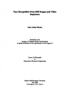
Figure 2. Different IR’s with the same minimal PE.
F RR
∞
∼
y∈G c , z∈G ¬c
(7)
−∞
We can find an optimal threshold h∗T so that the verification error P E is minimized, as illustrated in Fig. 1. As most of the subspace learning algorithms find a subspace where p(h|0) and p(h|1) is maximally separated, the separation however may not be characterized by a minimized P E. And some assumptions have to be made about the data (e.g., Gaussian distribution, manifold smoothness, etc), which may not always be satisfied for real-world applications. For face identification, the probe image x from subject c is correctly identified if {h(x, y)|y ∈ G c }
ha because lim (1 − PF R (h))C−1 → . C→∞ 1, for h ≤ ha For Fig. 2-(b), we will have lim IR = 0, because C→∞
lim (1 − PF R (h))C−1 → 0, for ∀h.
C→∞
Therefore, it is not guaranteed that face identification performance is optimal in a subspace where the data distributions are maximally separated. The pattern of the distribution overlap plays an important role in the performance of face identification. In the next section, we present algorithms that find the optimal subspaces by optimizing PE and IR, respectively.
3. Optimizing Subspaces Given a training set, the optimal subspace A∗ and decision threshold h∗T for face verification can be obtained as (A∗ , h∗T ) = arg minA,hT {P E}, where P E is defined by Eq. 1 (or 3), 2, and 4 based on the training set. Similarly the optimal subspace for face identification can be obtained as A∗ = arg maxA {IR}, where
IR is defined by Eq. 5. The hope is that performance optimization on the training set can be generalized to the testing data. Noticing that P E and IR are not differentiable due to the step function f (·), we can re-define f (·) as ∂f 1 = with ∂u (1) Sigmoid function f (u) = 1+e−u/σ 1 σ f (u)(1−f (u)); f (u) → Π(u) for σ → 0. This function subdues outliers in the data and improves robustness. ∂f (2) Exponential function f (u) = eu/σ with ∂u = 1 σ f (u). f (u) puts increasing penalty on the classification errors if σ → 0. If the data contains no outliers, this function results in fast optimization. According to the chain rule of differentiation, we E(A,hT ) and ∂IR(A) once we define can calculate ∂P∂A,h ∂A T ) = ∂h(AX,AY . ∂A If we define the distance metric as a Euclidean distance, we have ∂h(x,y) ∂A
∂h(AX, AY ) ∂A :
= =
∂ kAX − AY k2 ∂A : 2(A(X − Y )(X − Y )t ) :T , (9)
where the colon operator ‘ : ‘ stands for the vectorization of a matrix. For correlation based distance measure, we have
Algorithm 1 OSFV(P, I, G, J , A0 ) 1: 2: 3: 4: 5: 6: 7: 8: 9: 10:
Initialize σ = σ1 . A = A0 . while A has not converged do hT ← func opt thres(PA , I, GA , J ). ∂P E(A,hT ) . A←A−α ∂A if σ > σ� then σ ← βσ, {0 < β < 1}. end if end while return A, hT
Algorithm 2 func opt thres(PA , I, GA , J ) 1: Compute pairwise face match scores H = {h(x, y)|x ∈ PA , y ∈ GA }, |H| = |PA | × |GA |. 2: Obtain pairwise match ground-truth G = {δ(Id(x) − Id(y))| x ∈ PA , y ∈ GA , Id(x) ∈ I, Id(y) ∈ J }, where δ(u) = 1 i.f.f. u = 0. 3: Obtain Hsorted by sorting H in a descending order; and obtain Gsorted by rearranging G according to the sorting order. 4: Compute the sequential false alarm rate F AR as the cumulative sum of the sequence Gsorted . 5: Compute the sequential true rejection rate T RR = 1 − F RR as the cumulative sum of 1 − Gsorted . F AR , T RR ← PT RR . 6: Normalize F AR ← P G
(1−G)
RR 7: Obtain the sequential error rates P E = F AR+1−T , which 2 corresponds to the sorted decision thresholds in Hsorted . 8: Obtain the index i∗ ← arg min(P E). 9: h∗T ← Hsorted (i∗ ). 10: return h∗T
∂ X T AT AY p } {1 − p ∂A : X T AT AY Y T AT AX which increases the chance of guiding the optimization aXY AXX T aXY AY Y T toward the global minima. = { + a3X aY aX a3Y While it is possible to optimize the decision threshold hT by gradient descent, we present an efficient algoA(Y X T + XY T ) T − }: , (10) rithm that obtains the globally optimal decision threshaX aY old in Alg. 2 following the idea of an efficient ROC genp p T T eration method in [5]. Suppose there are n image pairs T T X A AX, aY = Y A AY , and where aX = T T for performance evaluation, this algorithm generates an aXY = X A AY . ROC curve by sorting the distance scores and obtains It is straightforward to optimize P E and IR using ∂P E(A,hT ) the decision threshold that minimizes the verification gradient descent optimization methods once ∂A,hT error on the ROC curve in O(n log n) time. and ∂IR(A) are calculated, respectively. ∂A ∂h(AX, AY ) ∂A :
=
3.2. Optimal Subspace for Face Identification
3.1. Optimal Subspace for Face Verification We can now summarize the Optimal Subspace for Face Verification (OSFV) algorithm in Alg. 1. The algorithm takes the probe and gallery set of a training set as input, and finds a subspace A and an optimal threshold hT by optimizing the face verification score P E iteratively. An initial guess for A0 can be obtained using one of the state-of-the-art subspace learning algorithms, such as LDA, LPP, MFA, etc. The parameter σ for f (·) is initialized with a large σ1 , and is gradually reduced to a smaller σ� in a fashion similar to simulated annealing, so that the gradient search on the cost function is initially done on a smoothed cost surface,
Similarly, we summarize the Optimal Subspace for Face Identification (OSFI) algorithm in Alg. 3. The computation of ∂IR ∂A has to be carried out during the evaluation of IR (Eq. 5), as the gradients are accumulated only from the gallery image of each ID that I ∗ ) ) is closest to the probe image, i.e., ∂h(x,G = ∂h(x,y , ∂A ∂A ∗ I y = arg min{h(x, y)|y ∈ G }.
3.3. Parameterization We define [σ� , σ1 ] = [γ� , γ1 ] × median({h(x, y)|x ∈ PA0 , y ∈ GA0 }), so that we can conveniently parameterize the range of σ suitable for optimization independent of the magnitude of the data variations. The
Property C |G| |P| P/G diff. Ctr : Cte
Algorithm 3 OSFI(P, I, G, J , A0 ) 1: 2: 3: 4: 5: 6: 7: 8: 9:
Initialize σ = σ1 . A = A0 . while A has not converged do A ← A + α ∂IR . ∂A if σ > σ� then σ ← βσ, {0 < β < 1}. end if end while return A
Conceptually Optimal Subspace
0.7 FDA
Gallery for ID1 Probe for ID1 Gallery for ID2 Probe for ID2
0.6
0.5
0.4
0.3
0.2
γ=0.05 γ=0.35 γ=0.1 0
0.1
0.2
0.3
0.4
0.5
0.6
0.7
0.8
0.9
1
Figure 3. A toy example for OSFV (best viewed in color).
user can then choose the appropriate [γ� , γ1 ] for emphasis on either better generalization capability (when the training data is sparse and contains no outlier) or for better robustness (when the training data contains a large number of outliers). If f (·) is the sigmoid function, we empirically assign γ� = 0.001 and γ1 = 0.03. If f (·) is the exponential function, we empirically fix γ = γ� = γ1 = 0.2. We set α = 1 and β = 0.98.
4. Experiments 4.1. Toy Example Fig. 3 shows a toy data distribution of two subjects where the statistics of the galleries and that of the probes are consistently incoherent. The FDA subspace (the green arrow) achieves a suboptimal PE of 12%. Using an exponential function and Euclidian distance metric, we perform OSFV optimization with A0 initialized by the FDA subspace, with different γ selected from [0.05 0.5]. The obtained OSFV subspaces (indicated by black arrows) reduce P E to 0 if γ > 0.1, and approximate the conceptually optimal subspace (indicated by the red arrow) if γ is further increased.
4.2. Performance Evaluation for OSFV and OSFI 4.2.1
CASPEAL 1025 1025 5859 Pose 717:308
CMU-PIE 59 767 15340 Illum. 39:20
Table 2. Data Preparation. C is the number of subjects; |G| and |P| are the number of images in the gallery and probe set; P/G diff. describes the major appearance differences in gallery and probe sets; and Ctr : Cte is the ratio of subject number in the training set and testing set.
OSFV
0.8
FERET 1009 1760 1517 Expr. 706:303
Experimental Setup
We now evaluate our algorithms on subsets of three widely used face databases, the FERET database [19], the CAS-PEAL database [7], and the CMU-PIE database [22]. Some major properties of the prepared database subsets are listed in Table 2. For the FERET database, we consider the f a set (faces with regular expressions) as the gallery set and the set f b (faces with alternative expressions) as the
probe set. For the CAS-PEAL data, we only consider the faces under ambient lighting, and take the frontal faces (P M + 00) as the gallery set, and the faces with pose variations (P M ±22, P M ±30, P U +00, P D+00) as the probe set. Due to the fact that these data sets do not have significant illumination variations, we specify the distance metric to be Euclidean distance. For the CMU-PIE database, we only consider the face images captured in Illumination 2 setting, in which each subject’s face is captured with 13 poses, and 21 illuminations. We use the face images of 13 poses for each subject under frontal illumination (Flash f09) as the gallery set, and the faces under other illuminations (13 × 20 images) as the probe set. Considering there exists a huge illumination variation in the data, we adopt the correlation based distance measure, which has been shown to be a good metric for face recognition under illumination variations [13, 6]. Since there are 13 face images of different poses in the gallery set for each subject, the computation of FAR is defined by Eq. 3 when evaluating PE. The face images are cropped according to the manually labeled eye locations, rectified to image size 32×32, and normalized to zero mean and standard deviation after histogram equalization. As all the databases are well processed and contain few outliers, we specify f (·) to be the exponential function for the OSFV/I optimization. Finally, we split the data (the gallery and probe sets) into training sets and testing sets with non-overlapped subject identity according to the ratio Ctr : Cte (See Table 2). We obtain the OSFV/I subspaces by optimizing face verification/identification performance on the training set, and evaluate the performance on the testing set. We show both the optimized performance on the training set and the evaluated performance on the testing set, so that we can get insight regarding how well the performance gain on the training set can be generalized to the testing set. 4.2.2
The Results
We now apply the subspace learning algorithms (PCA [24], FDA [2], LPP [11], OLPP [4], MFA [28], NPE [10], and the proposed OSFI/V algorithms) to
PE(%) P CA F DA LP P OLP P MF A NP E OSF V ∗ OSF V
FERET Train Test 13.4 14.5 ∗ 7.8 11.7∗ 0.0 15.5 2.0 10.4 0.3 14.9 11.3 16.9 ∗ 2.9 8.6∗ 1.5 9.1
CAS-PEAL Train Test 23.1 23.4 ∗ 11.3 11.9∗ 1.7 4.9 4.7 6.1 1.6 5.5 3.4 5.9 ∗ 2.3 4.4∗ 1.7 3.9
CMU-PIE Train Test 12.0 13.0 ∗ 5.2 5.8∗ 2.1 6.6 12.3 15.9 2.5 4.5 5.8 8.9 ∗ 0.3 2.7∗ 0.1 3.1
IR(%) P CA F DA LP P OLP P MF A NP E OSF I ∗ OSF I
FERET Train Test 74.6 80.5 ∗ 92.5 93.1∗ 99.9 92.0 98.8 92.4 99.5 90.7 98.5 94.1 ∗ 99.9 95.6∗ 99.9 95.4
CAS-PEAL Train Test 42.6 48.2 ∗ 78.0 79.1∗ 98.8 94.5 84.2 83.8 96.0 90.7 98.2 95.4 ∗ 97.9 91.2∗ 98.8 95.8
CMU-PIE Train Test 85.8 88.3 ∗ 96.1 96.2∗ 99.2 93.0 84.0 78.9 97.8 95.4 96.4 94.5 100∗ 98.2∗ 100 97.4
Table 3. Face Verification Performance
Table 4. Face Identification Performance
learn the subspace model from the training set, and evaluate the face recognition performances (PE and/or IR) on the testing set. Since our intention is to show how OSFV/I can further optimize the subspaces, for fair comparison, we empirically fix the dimensions of the subspaces to 80 for all evaluated algorithms. We first evaluate the face verification performance of these algorithms and the results are shown in Table 3. Without OSFV optimization, OLPP, LPP, and MFA achieves the lowest PE on the testing set for FERET, CAS-PEAL, and CMU-PIE, respectively. We apply OSFV optimization initialized by FDA subspace for all three databases. The row of OSF V ∗ indicates that OSFV can consistently reduce the PE of FDA by on average 6.3% on the training set and 4.2% on the testing sets (e.g., the PE for the testing set of CAS-PEAL reduces from 11.9% to 4.4%). We then apply OSFV optimization initialized by a subspace that achieves the best performance on the testing set of each database (as indicated by the underscored PE’s). The row of OSF V shows that the PE of OLPP, LPP, and MFA can be further reduced by on average 1% for the training set and 1.2% for the testing set. We then carry out face identification performance evaluation and list the results in Table 4. Without OSFI optimization, NPE achieves the highest identification rate on the testing sets for both FERET and CAS-PEAL, and FDA achieves the best performance on CMU-PIE. The row of OSF I ∗ lists the OSFI optimization results initialized with the FDA subspace. It is shown that OSF I ∗ can consistently increase the IR of FDA to nearly 100% in all the training sets. And the performance on the testing set can also be boosted consistently by 2-3% for FERET and CMUPIE, and 12% for CAS-PEAL. We also perform OSFI optimization initialized by a subspace other than FDA that achieves the highest performance on the testing set of each database (indicated by the underscored IR’s). As indicated by the row of OSF I, though these algorithms have achieved near 100% identification rate on the training set, OSFV can further improve their performance by 1-2% consistently on both the training and the testing set. This margin, in our view, is large considering the fact that the base performances are already around 95%.
From the results, we summarize as follows: (1) For each training and testing set division, the performance improvement by the OSFV/I on the training set always generalizes to the testing set. (2) For each individual task, none of the stateof-the-art subspace learning algorithms we tested can achieve the best performance across all databases. The OSFV/I algorithm however can consistently improve their performances independent of the database. (3) For each individual database, none of the stateof-the-art subspace learning algorithms can achieve best performances for both the face verification and the face identification tasks. By directly optimizing the performance scores, the proposed OSFV and OSFI can always achieve the best performance for each specific task, respectively, with proper initialization. (4) Across both tables, a variety of five subspaces are utilized as the initialization of the OSFV/I optimization, and their performances are shown to be further improved. This indicates that it is practical to utilize the OSFV/I algorithms to further improve the performance of the other subspace based face recognizers for a specific face recognition task. 4.2.3
Recognition performances w.r.t. C
To verify our theoretical analysis in Sec. 2, we take the F DA, OSF V ∗ , and OSF I ∗ subspaces trained on the FERET and evaluate their P E and IR on subsets of the FERET testing set with the number of subjects increasing from 10 to 170. By randomly generating the testing subsets of different number of subjects 200 times, we are able to plot the statistics of P E and IR w.r.t. C in Fig. 4. Fig. 4-(a) shows that OSFV achieves smaller P E in general. While P E is not a function of C by definition (Eq. 4), we observe the mean of P E decreases when C is small. We believe it is because the estimation of p(h|0) and p(h|1) is biased when the data set is small. The estimation of P E stabilizes after C > 70. Fig. 4-(b) shows that IR in general decreases when C increases. However, OSFI resists this trend the best because it finds a subspace in which the overlap pattern of p(h|0) and p(h|1) is optimal for face identification. The IR of OSFV decreases the fastest though it achieves the lowest PE in Fig. 4-(a).
14
102
12
OSFI OSFV FDA
100
10 98 IR
PE
8 96
6 94
4
OSFI OSFV FDA
2 0
92
90
0
20
40
60 80 100 120 number of subjects
140
160
180
0
20
40
60 80 100 120 number of subjects
140
160
180
(b) IR (a) PE Figure 4. Performance w.r.t. the number of subjects C.
4.3. Face Verification for Airport Security Check-in For the purpose of improving airport security and speeding up the check-in process, it is desirable to develop a face verification system that automatically verifies the identity of a passenger in real time by comparing facial images captured by a video camera and a face image scanned from a government issued ID, such as a driver license. Such a system installed at a airport check-in gate can greatly reduce the workload of airport security officers. Based on this application scenario, we collected a face database of 464 subjects from volunteers at our local airport. In the database, the face image on the driver license of each passenger is scanned as gallery data, and 3-8 face images are captured by a video camera as probe data. Large appearance variations can be observed due to differences in illumination, aging, pose, and facial expression between the gallery and probe data. In particular, a majority of photo ID scans contain confounding artifacts on the faces (such as a seal) or textured waveforms overlaid by the ID card. These artifacts pose additional difficulties to the face verification task. Fig. 5 illustrates some sample data of three subjects. In [17], O’Toole made the observation that computers can achieve better face verification performance than humans under illumination variations. To get an idea on how good humans can perform face verification in our setting, we ask 10 human subjects to manually perform face verification tasks based on 100 same-person image pairs and 100 different-person image pairs randomly drawn from the data set. We find it takes on average 4 seconds for a human subject to evaluate a image pair, and the average PE is 22.6%. We then split the data into a training set and a testing set with non-overlapped person identity. The training set contains 348 gallery images and 1512 probe images for 348 subjects, and the testing set contains 116 gallery images and 458 probe images for 116 subjects. The faces are then rectified according to the eye locations detected by a commercial face detector [16]. As the textured waveforms contain mostly high frequency information that can be removed by anti-aliasing filtering when the images are downsized, we choose to down-
Figure 5. The airport check-in data: The scanned ID face images (the first row) and the corresponding face image captured by a video camera (the second row). PE(%) P CA F DA F DA LP P OLP P MF A NP E OSF V ∗ OSF V Human
#Dim 150 400 50 50 50 550 350 50 50 —
Train 25.7 4.2 17.9∗ 1.8 15.5 6.1 23.1 9.0∗ 1.3 —
Test 28.0 22.9 24.3∗ 22.1 28.9 22.4 26.1 19.0∗ 21.7 22.6
Table 5. Face verification for airport check-in.
size the rectified face images to size 32 × 32. Several state-of-the-art subspace learning algorithms are then applied to learn the models from the training data, and their face verification performances are then evaluated on the testing data. By varying the number of dimensions of the subspaces from 30 to 600, we report the lowest PE on the testing set for each algorithm w.r.t the subspace dimension number. The results are shown in Table 5. The best performance on the testing set is achieved by LPP subspace with 50 dimensions. We now perform OSFV optimization. As there exist substantial outliers and illumination variations in the data, we specify f (·) to be the sigmoid function and adopt normalized correlation based distance metric. Noticing the FDA subspace of 50 dimensions performs just slightly worse than the FDA subspace of 400 dimensions. We initialize the OSFV optimization by the FDA subspace of 50 dimensions. The performances shown in the row of OSF V ∗ indicate that OFSV reduces the PE by 5% on the testing set. We then apply the OSFV optimization initialized by the LPP subspace. The face verification performance is also improved, but not as much as when initialized by the FDA subspace. Overall, we find most of the subspace learning algorithms can not exceed the performance of human (and LPP and MFA perform barely better than human), probably due to the existence of large amount of outliers in the data. And the OSFV subspace optimization is able to reduce the PE to 19% which is 3.9% better than the human performance.
5. Conclusion We proposed a novel OSFV/I algorithm that directly optimizes the performance scores of various face recognition tasks. The algorithm in nature takes into consideration the differences of the performance score definitions of the different tasks and the intrinsic appearance incoherences between the gallery images and the probe images of the same subject caused by the data collection procedures in real-world applications. In the experiments on the FERET, CAS-PEAL and CMU-PIE database, we demonstrated how the proposed OSFV/I algorithms can further improve the performance of the state-of-the-art subspace learning algorithms on both the training set and the testing set. And we presented its successful application to a new real-world database we collected for the airport checkin face verification task. Our theoretical analysis and experiments verified several points that were not emphasized by prior face recognition work: There exists different optimal face subspaces for different face recognition tasks. And there could exists consistent appearance incoherences in the gallery and the probe set in real-world applications. By customizing the algorithm design specific for a face recognition task and taking advantage of the knowledge in the consistent appearance incoherence in the gallery and probe set, the performance of the existing subspace based face recognition algorithm can be further improved. While these points are made in the context of subspace based face recognition, our future work is to study how they can be extended to other types of face recognizers (such as boosting, SVM, etc.).
Acknowledgement This work was supported by award #2007-DEBX-K191 from the National Institute of Justice, Office of Justice Programs, US Department of Justice. The opinions, findings, and conclusions or recommendations expressed in this publication are those of the authors and do not necessarily reflect the views of the Department of Justice. We also appreciate Dr. Deng Cai for sharing his subspace learning matlab code at http://www.cs.uiuc.edu /homes/dengcai2/Data/data.html.
References [1] M. Bartlett, H. Lades, and T. Sejnowski. Independent component representations for face recognition. In SPIE, volume 3299, pages 528–539, 1998. [2] P. Belhumeur, J. Hespanha, and D. Kriegman. Eigenfaces vs. Fisherfaces: Recognition using class specific linear projection. In ECCV, pages 45–58, 1996. [3] M. Belkin and P. Niyogi. Laplacian eigenmaps and spectral techniques for embeddings and clustering. In NIPS, pages 585– 591, 2002.
[4] D. Cai, X. He, J. Han, and H.-J. Zhang. Orthogonal Laplacianfaces for face recognition. IEEE TIP, 15(11):3608–3614, 2006. [5] T. Fawcett. ROC graphs: Notes and practical considerations for researchers. Technical report, HP Laboratories, 2004. [6] Y. Fu, S. Yan, and T. Huang. Correlation metric for generalized feature extraction. IEEE TPAMI, 30(12):2229–2235, 2008. [7] W. Gao, B. Cao, S. Shan, X. Chen, D. Zhou, X. Zhang, and D. Zhao. The CAS-PEAL large-scale Chinese face database and baseline evaluations. IEEE TSMC, 38(1):149–161, 2008. [8] J. Goldberger, S. Roweis, G. Hinton, and R. Salakhutdinov. Neighbourhood components analysis. In L. K. Saul, Y. Weiss, and L. Bottou, editors, NIPS, pages 513–520, Cambridge, MA, 2005. MIT Press. [9] O. Hamsici and A. Martinez. Bayes optimality in linear discriminant analysis. IEEE TPAMI, 30(4):647–657, 2008. [10] X. He, D. Cai, S. Yan, and H.-J. Zhang. Neighborhood preserving embedding. In ICCV, volume 2, pages 1208–1213. [11] X. He and P. Niyogi. Locality preserving projections. In NIPS, 2003. [12] M. Kirby and L. Sirovich. Application of the Karhunen-Loeve procedure for the characterization of human faces. IEEE TPAMI, 12(1):103–108, 1990. [13] B. V. K. V. Kumar, A. Mahalanobis, and R. Juday. Correlation Pattern Recognition. Cambridge University Press, 2006. [14] S. Z. Li and A. K. Jain. Springer, 2005.
Handbook of Face Recognition.
[15] B. Moghaddam, T. Jebara, and A. Pentland. Bayesian face recognition. Pattern Recognition, 33(11):1771–1782, 2000. [16] M. C. Nechyba, L. Brandy, and H. Schneiderman. Multimodal Technologies for Perception of Humans, volume 4625, chapter PittPatt Face Detection and Tracking for the CLEAR 2007 Evaluation, pages 126–137. Springer Berlin / Heidelberg, 2008. [17] A. O’Toole, P. Phillips, F. Jiang, J. Ayyad, N. Penard, and H. Abdi. Face recognition algorithms surpass humans matching faces over changes in illumination. IEEE TPAMI, 29(9):1642– 1646, 2007. [18] V. Perlibakas. Distance measures for pca-based face recognition. Pattern Recognition Letter, 25:711–724, 2004. [19] P. J. Phillips, H. Moon, P. J. Rauss, and S. Rizvi. The FERET evaluation methodology for face recognition algorithms. IEEE TPAMI, 22(10):1090–1104, 2000. [20] J. G. Proakis and M. Salehi. Communication Systems Engineering. Prentice-Hall, Inc., 1994. [21] S. Roweis and L. Saul. Nonlinear dimensionality reduction by locally linear embedding. Science, 290(5500):2323–2326, 2000. [22] T. Sim, S. Baker, and M. Bsat. The CMU pose, illumination, and expression database. IEEE TPAMI, 25(12):1615–1618, 2003. [23] J. B. Tenenbaum, V. de Silva, and J. Langford. A global geometric framework for nonlinear dimensionality reduction. Science, 290(5500):2319–2323, 2000. [24] M. Turk and A. Pentland. Eigenfaces for recognition. Journal of Cognitive Neurosicence, 3(1):71–86, 1991. [25] M. Villegas and R. Paredes. Simultaneous learning of a discriminative projection and prototypes for nearest-neighbor classification. In CVPR, 2008. [26] H. Wechsler, P. J. Philips, V. Bruce, F. F. Soulie, and T. huang, editors. Face Recognition: From Theory to Applications. Springer-Verlag Berlin and Heidelberg GmbH & Co. K. [27] S. Yan, J. Liu, X. Tang, and T. Huang. Formulating face verification with semidefinite programming. IEEE TIP, 16:2802– 2810, 2007. [28] S. Yan, D. Xu, B. Zhang, and H. Zhang. Graph embedding: A general framework for dimensionality reduction. In CVPR, volume 2, pages 830–837, 2005.