On Quantitative Evaluation of Clustering Systems Contents - CiteSeerX

Information Retrieval and Clustering W. Wu and H. Xiong (Eds.) pp. – - – c

2002 Kluwer Academic Publishers

On Quantitative Evaluation of Clustering Systems Ji He School of Computing, National University of Singapore 3 Science Drive 2, Singapore 117543 E-mail: [email protected]

Ah-Hwee Tan Laboratories for Information Technology 21 Heng Mui Keng Terrace, Singapore 119613 E-mail: [email protected]

Chew-Lim Tan School of Computing, National University of Singapore 3 Science Drive 2, Singapore 117543 E-mail: [email protected]

Sam-Yuan Sung School of Computing, National University of Singapore 3 Science Drive 2, Singapore 117543 E-mail: [email protected]

Contents 1 Introduction

2

2 Clustering Process: A Brief Review 2.1 Pattern Representation, Feature Selection and Feature Extraction . 2.2 Pattern Proximity Measure . . . . . . . . . . . . . . . . . . . . . . . 2.3 Clustering Algorithms . . . . . . . . . . . . . . . . . . . . . . . . . .

3 3 5 6

3 Evaluation of Clustering Quality 3.1 Evaluation Measures Based on Cluster Distribution . . . . . . . . . . 3.2 Evaluation Measures Based on Class Conformation . . . . . . . . . .

7 9 11

1

4 Clustering Methods 13 4.1 k-means . . . . . . . . . . . . . . . . . . . . . . . . . . . . . . . . . . 13 4.2 Self-Organizing Maps (SOM) . . . . . . . . . . . . . . . . . . . . . . 14 4.3 Adaptive Resonance Theory under Constraints (ART-C) . . . . . . . 15 5 Experiments and Discussions 5.1 Statistical Validation of Comparative Observation 5.2 Identification of the Optimal Number of Clusters . 5.3 Selection of Pattern Proximity Measure . . . . . . 5.4 Cross-Comparison of Clustering Methods . . . . . 5.4.1 Data Preparation . . . . . . . . . . . . . . . 5.4.2 Evaluation Paradigm . . . . . . . . . . . . . 5.4.3 Results and Discussions . . . . . . . . . . . 6 Conclusions

. . . . . . .

. . . . . . .

. . . . . . .

. . . . . . .

. . . . . . .

. . . . . . .

. . . . . . .

. . . . . . .

. . . . . . .

. . . . . . .

18 18 19 20 21 22 22 23 26

References

1

Introduction

Clustering refers to the task of partitioning unlabelled data into meaningful groups (clusters). It is a useful approach in data mining processes for identifying hidden patterns and revealing underlying knowledge from large data collections. The application areas of clustering, to name a few, include image segmentation, information retrieval, document classification, associate rule mining, web usage tracking, and transaction analysis. While a large number of clustering methods have been developed, clustering remains a challenging task as a clustering algorithm behaves differently depending on the chosen features of the data set and the parameter values of the algorithm [10]. Therefore, it is important to have some objective measures to evaluate the clustering quality in a quantitative manner. Given a clustering problem with no prior knowledge, a quantitative assessment of the clustering algorithm serves as an important reference for various tasks, such as discovering the distribution of a data set, identifying the clustering paradigm that is most suitable for a problem domain, and deciding the optimal parameters for a specific clustering method. In the rest of this chapter, we review the process of clustering activities and discuss the factors that affect the output of a clustering system. We then describe two sets of quality measures for the evaluation of clustering algorithms. While the first set of measures evaluate clustering outputs in 2

terms of their inherent data distribution, the second set evaluates output clusters in terms of how well they follow known class distribution of the problem domain. We illustrate the application of these evaluation measures through a series of controlled experiments using three clustering algorithms.

2

Clustering Process: A Brief Review

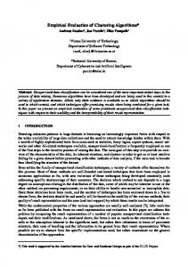
Jain et al summarized a typical sequence of the clustering activities as the following three stages depicted in Figure 1 [13, 14]: 1. pattern representation, optionally including feature extraction and/or selection, 2. definition of a pattern proximity measure for the data domain, and 3. clustering or grouping of data points according to the chosen pattern representation and the proximity measure.

Patterns

Feature Selection / Extraction

Pattern Representation

Interpattern Similarity

Grouping

Clusters

Feedback Loop

Figure 1: A typical sequencing of clustering activity. Since the output of a clustering system is the result of the system’s interactive activities in each stage, various factors in each stage that affect the system’s activity in turn have impact on the clustering output. We extend our discussion in the following subsections.

2.1

Pattern Representation, Feature Selection and Feature Extraction

Pattern representation refers to the paradigm for observation and the abstraction of the learning problem, including the type, the number and the scale of the features, the number of the patterns, and the format of the feature representation. Feature selection is defined as the task of identifying a set of most representative subset of the natural features (or transformations of the natural features) to be used by the machine. Feature extraction, on 3

the other hand, refers to the paradigm for converting the observations of the natural features into a machine understandable format. Pattern representation is considered as the basis of machine learning. Since human accessibility of the patterns is highly dependent on their representation format, an unsuitable pattern representation may result in a failure of producing meaningful clusters as a user desires. As show in Figure 2a, using a cartesian coordinate representation, a clustering method would have no problem in identify the five compact groups of data points. However, when the same representation is applied to the data set in Figure 2b, the four string-shape clusters would probably not be discovered as they are not easily separable, in terms of Euclidean distance. Instead, a polar coordinate representation could lead to a better result, as the data points in each string-shape cluster are close to each other, in terms of polar angle. 1

1

0.5

0.5

0

0

0.5

0

1

(a)

0

0.5

1

(b)

Figure 2: To identify compact clusters, a cartesian coordinate representation is more suitable for case (a), while a polar coordinate representation is more suitable for case (b). Feature selection and extraction play an important role for abstracting complex patterns into a machine understandable representation. The feature set used by a clustering system regularizes the “area” that the system gives “attention” to. Referring to the data set in Figure 2a, if coordinate position is selected as the feature set, many clustering algorithms would be capable of identifying the five compact clusters. However, if only the color of the data points is selected as the feature, a clustering system would probably output 4

only two clusters, containing white points and black points respectively. The feature set also affects the quality as well as the efficiency of a clustering system. A large feature set containing numerous irrelevant features does not improve the clustering quality but increases the computational complexity of the system. On the other hand, an insufficient feature set may decrease the accuracy of the representation and therefore cause potential loss of important patterns in the clustering output.

2.2

Pattern Proximity Measure

Pattern proximity refers to the metric that evaluates the similarity (or in contrast, the dissimilarity/distance) between two patterns. While a number of clustering methods (such as [17]) disclaim the use of specific distance measures, they use alternative pattern proximity measures to evaluate the so-called relationship between two patterns. A pattern proximity measure serves as the basis for cluster generation as it indicates how two patterns “look alike” to each other. Since the type, the range, and the format of the input features are defined during the pattern representation stage, it follows that a pattern proximity measure should correspond to the pattern representation. In addition, a good proximity measure should be capable of utilizing only the key features of the data domain. Referring to Figure 2 again, with a cartesian representation, Euclidean distance is suitable to identify the geometric differences among the five clusters in data set (a) but may not be capable enough to recognize the clusters in data set (b). Instead, cosine distance is more suitable for data set (b), as it gives no weight to a vector’s radius and focuses on the differences of the vectors’ projections on the polar angle only. Generally, a careful review on the existing correlations among patterns helps to choose a suitable pattern similarity measure. Given an existing pattern representation paradigm, a data set may be separable in various ways. Under this condition, using different pattern proximity measures may result in very different clustering outputs. Figure 3 depicts a simple example using eight speed cameras on three roads. Based on different proximity criteria listed in Table 1, there are different solutions for clustering the speed cameras, each with an acceptable interpretation. In most cases, the clustering system is desired to output only one (or a few number of) optimal grouping solution that best matches the user intention on the data set, although that may be partial and subjective. Hence it is important to identify the pattern proximity measure that effectively and precisely formulates the user’s intention on the patterns. 5

S7

S5 S1 S3

S8

S2 S4

S6

Figure 3: Using various pattern proximity measures, the eight speed cameras on the three roads may be clustered into different cluster groupings. Table 1: Interpretations to the various clustering results of the eight speed cameras, based on different pattern proximity measures. Measure Geometric distance Connectivity

Density

2.3

Clustering Result C1 = {S1 , S2 , S3 , S4 , S5 } C2 = {S6 , S8 } C3 = {S7 } C1 = {S1 , S2 , S3 , S4 } C2 = {S5 , S6 } C3 = {S7 , S8 } C1 = {S1 , S2 , S3 , S4 , S5 } C2 = {S6 , S7 , S8 }

Interpretation Cameras in each cluster are geometrically closer to each other than to those in other clusters. Each cluster contains the cameras in the same road. C1 identifies the zone intensively equipped with cameras, in contrast to the rest of the area.

Clustering Algorithms

A clustering algorithm groups the input data according to a set of predefined criteria. The clustering algorithm used by a system can be either statistical or heuristic. In essence, the objective of clustering is to maximize the intra-cluster similarity and minimize the inter-cluster similarity [23]. A large variety of clustering algorithms have been extensively studied in the literature. While a comprehensive survey of clustering algorithms is not the focus of our study, we give a bird’s-eye review of various types of the available algorithms in Table 2. 6

Table 2: Various types of clustering methods, based on learning paradigm, codebook size, cluster assignment, and system architecture respectively. Criteria Learning paradigm

Codebook size (number of output clusters) Cluster assignment

System architecture

Categories Off-line: Iteratively batch learning on the whole input set. On-line: Incremental learning that does not remember the specific input history. Static-sizing: The codebook size is fixed. Dynamic-sizing: The codebook size is adaptive to the distribution of input data. Hard: Each input is assigned with one class label. Fuzzy: Each input is given a degree of membership with every output cluster. Partitioning: The input space is naively separated into disjoint output clusters. Hierarchical: The output tree shows the relations among clusters. Density-based: The input data are grouped based on density conditions. Grid-based: The spacial input space is quantized into finite sub-spaces (grids) before clustering of each sub-space.

Despite the numerous clustering algorithms available in the literature, there is no single method that can cope with all clustering problems. The choice of the clustering algorithm for a specific task affects the clustering result in a fundamental way. In addition, the learning activity of a large number of clustering algorithms is controlled and hence affected by a set of internal parameters. The optimal parameter set is usually decided through empirical experiments on the specific data set.

3

Evaluation of Clustering Quality

With the summarization of the various factors that affect the result of a clustering system, it is desirable for a clustering system to be capable of providing the necessary feedback to each stage of the clustering process, based on the evaluation and the interpretation of the clustering output. Such 7

a feedback helps to gather prior knowledge on the data distribution, define a suitable pattern proximity measure that matches the problem domain, choose a clustering algorithm as well as decide the optimal parameter setting for the specific algorithm, and therefore lead to an optimal clustering output. Human inspection on the clustering output may be the most intuitive clustering validation method as it compares the clustering result with the user’s intention in a natural way. In fact, human inspection has been widely used to validate the clustering outputs of the controlled experiments on two dimensional data sets. However, human inspection lacks the scalability to high dimensional, large, and complicated problem domains. In addition, manual inspection is always not desirable and not feasible in real-life applications. Therefore, quantitative assessment of clustering quality is of great importance for various clustering applications. When talking about quantitative measure of the clustering quality, readers should be aware that the definition of the quality actually is quite subjective. Given an input data set, users may have varying desires on the knowledge that a clustering system could discover, and therefore give different interpretation of the clustering quality. Before a quality measure is applied to evaluate the clustering results generated by two different systems, a study on the quantitative comparability of the outputs is fundamentally important. We consider two clustering systems quantitative comparable only if: • the pattern representation of the two systems are similar enough, • they are based on the similar clustering fundament, and • they intend to fulfill the same user requirement, optionally to optimize the same criteria. We give explanations through examples below. Given the speed camera example as in Figure 3, the three clustering results in Table 1 are not quantitatively comparable as they are based on different clustering criteria. Likewise, given the data set as in Figure 2a, the clustering output based on the coordinate position of each data point is not quantitatively comparable with that based on the color of each data point, as they are based on totally different feature sets. However, using the same feature representation (coordinate position), the outputs of the two clustering methods as in Figure 4 are quantitatively comparable as they both attempt to identify compact clusters of the data set. A multitude of clustering evaluation measures have been extensively studied in the literature. Examples include the Dunn and Dunn-like family 8

1

1

0.5

0.5

0

0

0.5

0

1

(a)

0

0.5

1

(b)

Figure 4: Two quantitatively comparable partitioning outputs of the data set in Figure 2a. Each type of marker identifies data points in the same cluster. Result (a) is considered to have a higher quality than result (b) in the sense that it recognizes the large cluster (marked with solid circles in (a)) more precisely. of measures initially proposed for evaluation of crisp [7], the variances of DB measures [6, 16], the various cross validation methods based on Monte Carlo theory [18], and the relatively recent SD validity indices [11]. However, due to the limitations mentioned above, a large number of these evaluation measures are capable of validating a narrow ranges of in-house clustering methods only. Our study intents to use a set of evaluation measures with high scalability, in terms of the capability for evaluating a wide range of clustering systems. In the rest of this section, we introduce several clustering evaluation measures based on two different statistical fundaments, i.e. cluster distribution and class conformation respectively.

3.1

Evaluation Measures Based on Cluster Distribution

The objective of clustering has been widely quoted as to reorganize the input data set in an unsupervised way such that data points in the same cluster are more similar to each other than to points in different clusters. When explaining this objective in the quantitative manner, it is to minimize the distances among the data points in individual clusters and to maximize the 9

distances between clusters. Therefore, it is a natural way to validate the intra-cluster homogeneity and the inter-cluster separation of the clustering output in a global fashion, using the quantities inherent to the distribution of the output data. We extend our study from the various clustering validity methods in this category [9, 11], and propose two quality evaluation measures, namely: cluster compactness and cluster separation. The definitions of these measures are given as below. Cluster Compactness: The cluster compactness measure introduced in our study, is based on our generalized definition of the variance of a vector data set given by v u N u1 X d2 (xi , x) v(X) = t

N

(1)

i=1

where d(xi , xj ) is a distance metric between two vectors xi and xj , N is the P number of members in X, and x = N1 i xi is the mean of X. A smaller variance value of a data set indicates a higher homogeneity of the vectors in the data set, in terms of the distance measure d(). Particularly, when X is one-dimensional and d() is the Euclidean distance, v(X) becomes the statistical variance of the data set σ(X). The cluster compactness for the output clusters c1 , c2 , · · · , cC generated by a system is then defined as Cmp =

C v(ci ) 1 X , C i v(X)

(2)

where C is the number of clusters generated on the data set X, v(ci ) is the variance of the cluster ci , and v(X) is the variance of the data set X. The cluster compactness measure evaluates how well the subsets (output clusters) of the input is redistributed by the clustering system, compared with the whole input set, in terms of the data homogeneity reflected by the distance metric used by the clustering system. When the distance metric is the Euclidean distance, the cluster compactness measure becomes coherent to the average cluster scattering index used in Halkidi et al’s study [11]. It is understandable that, for the cluster compactness measure, a smaller value indicates a higher average compactness in the output clusters. This however does not necessarily mean a “better” clustering output. Given a clustering system that encodes each and every unique input data into one separate cluster, the cluster compactness score of its output has a minimal value of 0. Such a clustering output is however not desirable. To tackle this, we introduce the cluster separation measure to complement the evaluation. 10

Cluster Separation: The cluster separation measure introduced here borrows the idea in [11] and combines the idea of the clustering evaluation function introduced by [9]. The cluster separation of a clustering system’s output is defined by Sep =

C C X X d2 (xci , xcj ) 1 exp(− ), C(C − 1) i=1 j=1,j6=i 2σ 2

(3)

where σ is a Gaussian constant, C is the number of clusters, xci is the centroid of the cluster ci , d() is the distance metric used by the clustering system, and d(xci , xcj ) is the distance between the centroid of ci and the centroid of cj . It is noted that the pair-wise distances among the output cluster centroids are the key components of the cluster separation measure. The Gaussian function and the L1-normalization normalizes its value to between 0 and 1. A smaller cluster separation score indicates a larger overall dissimilarity among the output clusters. However, given the particular case that a clustering system output the whole input set into one cluster, the cluster separation score reaches to minimal value of 0, which is not applicably desirable. Hence, we reach the necessary point to combine the cluster compactness and cluster separation measures into one in order to tackle each one’s deficiency and evaluate the overall performance of a clustering system. An intuitive combination, named overall cluster quality, is defined as: Ocq(β) = β · Cmp + (1 − β) · Sep,

(4)

where β ∈ [0, 1] is the weight that balances measures cluster compactness and cluster separation. Particularly, Ocq(0.5) gives equal weights to the two measures. Readers however should be aware of the limitation of this combination: although the combination measure Ocq facilitates the comparison work, one may find it not easy to interpret the combined value, as the Cmp and Sep scores are not measured in the same dimension. In addition, in some other cases, evaluating a clustering system through intra-cluster compactness and inter-cluster separation respectively helps to gain more insightful understanding of the system characteristics.

3.2

Evaluation Measures Based on Class Conformation

This category of validation measures assumes that there is a desirable distribution of the data set with which it is possible to perform a direct comparison of the clustering output. Following the data distribution, one can assign a 11

class label to each data point. The target of the clustering system can then be correspondingly interpreted as to replicate the underlying class structure through unsupervised learning. In an optimal clustering output, data points with the same class labels are clustered into the same cluster and data points with different class labels appear in different clusters. We describe two quantitative evaluation measures based on these criteria as follows. Cluster Entropy: Boley [1] introduced an information entropy approach to evaluate the quality of a set of clusters according to the original class labels of the data points . For each cluster ci , a cluster entropy Eci is computed by X n(lj , ci ) n(lj , ci ) log (5) Eci = − n(ci ) n(ci ) j where n(lj , ci ) is the number of the samples in cluster ci with a predefined P label lj and n(ci ) = j n(lj , ci ) is the number of samples in cluster ci . The overall cluster entropy Ec is then given by a weighted sum of individual cluster entropies by Ec = P

X 1 n(ci )Eci . i n(ci ) i

(6)

The cluster entropy reflects the quality of individual clusters in terms of homogeneity of the data points in a cluster (a smaller value indicates a higher homogeneity). It however does not measure the compactness of a clustering solution in terms of the number of clusters generated. A clustering system that generates many clusters would tend to have very low cluster entropies but is not necessarily desirable. To counter this deficiency, we use another entropy measure below to measure how data points of the same class are represented by the various clusters created. Class Entropy: For each class lj , a class entropy Elj is computed by Elj = −

X n(lj , ci ) i

n(lj )

log

n(lj , ci ) n(lj )

(7)

where n(lj , ci ) is the number of samples in cluster ci with a predefined label P lj and n(lj ) = i n(lj , ci ) is the number of the samples with class label lj . The overall class entropy El is then given by a weighted sum of individual class entropies by X 1 El = P n(lj )Elj . (8) j n(lj ) j

Since both the cluster entropy and class entropy utilize the predefined class labels on the input data only, they are independent to the choice of the 12

feature representation and the pattern proximity measure. Therefore these two measures are practically capable of evaluating any clustering system. Compared with the cluster distribution based measures, these class conformation based measures are likely to have more advantages for identifying the optical clustering solution to match the user’s intention on the problem domain. One apparent drawback however is the potential complexity of the labelling process, which may not be feasible and not desirable in real-life applications. Our prior study showed that, similar to the characteristics of the cluster compactness and the cluster separation measures, as the number of clusters over one data set increases, the cluster entropy generally decreases while the class entropy increases. We follow the identical paradigm for the combination of cluster compactness and cluster separation, and define a combined overall entropy measure: Ecl(β) = β · Ec + (1 − β) · El,

(9)

where β ∈ [0, 1] is the weight that balances the two measures.

4

Clustering Methods

Before introducing our experiments on the various clustering quality measures, review of the clustering systems used in our experiments helps toward a better understanding of the experimental results. Our experiments tested three partitioning methods that work with a fixed number of clusters, namely k-means [19], Self-Organizing Maps (SOM) [15], and Adaptive Resonance Theory under Constraints (ART-C) [12]. The learning algorithms of the three methods are summarized as follows.

4.1

k-means

k-means [19] has been extensively studied and applied in the clustering literature due to its simplicity and robustness. The fundament of the k-means clustering method is to minimize the intra-cluster compactness of the output, in terms of the summed squared error. The k-means clustering paradigm is summarized below. 1. Initialize the k reference clusters with randomly chosen input points or through certain estimation of the data distribution. 2. Assign each input point to the nearest cluster centroid. 13

3. Recalculate the centroid of each cluster using the mean of the input points in the cluster. 4. Repeat from step 2 until convergence. Since k-means follows a batch learning paradigm to iteratively adjust the cluster centroids, it is inefficient in handling large scale data sets. In addition, the output of k-means is affected by the cluster initialization method. Its strength however lies in the satisfactory quality in the sense that the output has locally minimal summed squared error when it converges.

4.2

Self-Organizing Maps (SOM)

SOM as proposed by Kohonen [15] is a family of self-organizing neural networks widely used for clustering and visualization. As an unique feature of SOM, the clusters in a SOM network are organized in a multi-dimensional map. During learning, the network updates not only the winner’s weight, but also the weights of the winner’s neighbors. This results in an output map with a distribution that similar patterns (clusters) are placed together. The learning paradigm of SOM is given below. (0)

1. Initialize each reference cluster wj with random values. Set the initial (0)

neighborhood set of each cluster Nj

to be large.

2. Given an input xi , find the winner node J that has the maximal similarity with xi . 3. Update the cluster vectors of the winner node and its neighbors, according to (t+1)

wj

(t)

(t)

(t)

= wj + η (t) h(j, J)(xi − wj ) for each j ∈ NJ ,

(10)

where h(j, J) ∈ [0, 1] is a scalar kernel function that gives a higher weight to a closer neighbor of the winner node J and η (t) is the learning rate. 4. At the end of the learning iteration, shrink the neighborhood sets so (t+1) (t) that Nj ⊂ Nj for each j and decrease the learning rate so that η (t+1) < η (t) . Repeat from step 2 until convergence. There are a large number of SOM variances depending on the dimension of the organization map, the definition of the neighborhood sets Ni , 14

the kernel function h(), as well as the paradigm that iteratively readjusts Ni and η. When the network utilizes one-dimensional map and the degree of neighborhood is zero (i.e. the neighborhood contains the winner node only), SOM equals to an online learning variance of the k-means clustering method [8]. It is also understandable that, if the neighborhood degree shrinks to zero at the end of the learning, SOM is capable of obtaining optimal output with locally minimal summed square error. The drawback of SOM is that its learning activity is affected by the initialization of network and the presentation order of the input data.

4.3

Adaptive Resonance Theory under Constraints (ART-C)

ART-C [12] is a new variance of the Adaptive Resonance Theory (ART) neural networks, which was originally developed by Carpenter and Grossberg [5]. Unlike the conventional ART modules which work on a dynamic number of output clusters, an ART-C module is capable of satisfying a user constraint on its codebook size (i.e. the number of output clusters), while keeping the stability-plastically of ART intact. Compared with the conventional ART architecture, the ART-C architecture (Figure 5) contains an added constraining subsystem, which interacts with the ART’s attentional subsystem and the orienting subsystem. During learning, the constraining subsystem adaptively estimates the distribution of the input data and selfadjusts the vigilance parameter for the orienting subsystem, which in turn governs the learning activities in the attentional subsystem. The learning paradigm of ART-C is summarized below. Attentional Subsystem

+

F2

Constraining

C Subsystem

-

F1

ρ

-

…

Orienting Subsystem

+

F0 Input

Figure 5: The ART-C architecture.

15

1. Initialize the network’s recognition layer F2 with null set ø (i.e. the number of clusters in F2 is zero) and set the network’s vigilance ρ as 1.0. 2. Given an input xi in the input layer F0 , the comparison layer F1 stores the match scores M (xi , wj ) between the input and every cluster vector wj in F2 . 3. If the maximal match scores satisfies max{M (xi , wj )} ≥ ρ or the number of clusters c in F2 satisfies c < C, where C is the user constraint on the number of output clusters, then carry out the conventional ART learning process, which is summarized below, (a) Calculate the choice scores T (xi , wj ) between the input and every cluster vector wj in F2 . (b) Identify the winner node J that receives the maximal choice score T (xi , wJ ). Resonance happens when the match score M (xi , wJ ) ≥ ρ. Otherwise reset the winner node J and repeat the search process. (c) If the network reaches resonance, the network updates the cluster vector of the winner node, according to a learning function (t+1)

wJ

(t)

= L(xi , wJ ).

(11)

Otherwise, if all F2 nodes j are reset, insert the input xi into the F2 layer as a new reference cluster. otherwise, do constraint reset, which is summarized below, (a) Insert input xi into F2 layer as a new reference cluster. (b) Calculate the pair wise match score M (wi , wj ) of every F2 node pairs. (c) Locate the winner pair (I, J) according to M (wI , wJ ) = max{M (wi , wj ) : i ∈ R},

(12)

where R is the set of F2 nodes indexed by the criteria: R = {F2 node i whose max{M (wi , wj ) : j 6= i} < ρ}. 16

(13)

(d) Modify the network’s vigilance according to the match score between the winner pair: ρnew = M (wI , wJ ).

(14)

(e) Update wJ with wI , by utilizing the ART learning function: (t+1)

wJ

(t)

(t)

= L(wI , wJ ).

(15)

(f) Delete node I from F2 layer. 4. Repeat from step 2 until convergence. The ART module used in the ART-C architecture can be either ART-1 [5], ART-2 [2, 4] or fuzzy ART [3], each using a different set of choice, match, and learning functions. ART-2 utilizes the cosine similarity as the choice and match functions: xi · w j T (xi , wj ) = M (xi , wj ) = , (16) ||xi ||||wj || where the L2 -norm function || · || is defined by ||x|| =

sX

x2i

(17)

i

for vector x. The learning function is given by L(xi , wj ) = ηxi + (1 − η)wj .

(18)

where η is the learning rate. As a comparison, fuzzy ART uses hyperrectangle based choice and match functions T (xi , wj ) =

|xi ∧ wj | , α + |wj |

(19)

M (xi , wj ) =

|xi ∧ wJ | , |xi |

(20)

where α is a constant, the fuzzy AND operation ∧ is defined by (p ∧ q)i ≡ min(pi , qi )

(21)

and the L1-norm |.| is defined by |p| ≡

X i

17

pi

(22)

for vectors p and q. The learning function for fuzzy ART is given by L(xi , wj ) = η(xi ∧ wj ) + (1 − η)wj .

(23)

ART-C adaptively generates reference clusters (recognition categories) using the input samples. Therefore no prior knowledge on the data distribution is required for the initialization of the network. However, like most online learning algorithms, ART-C’s learning is affected by the presentation order of the input data.

5

Experiments and Discussions

The experiments reported in this section illustrate the use of the various clustering evaluation measures for a variety of purposes. We extend our discussion on the two synthetic data sets as in Figure 2a and 2b in a quantitative manner. Tasks on these two data sets include identifying the optimal number of clusters in the data set and choosing of a pattern proximity measure suitable for the specific data distribution. In addition, using a highdimensional and sparse real-life data set, i.e. the Reuters-21578 free text collection, we carry out comparisons across the performance of three distinct clustering algorithms, namely k-means, SOM, and ART-C, to discover the similarities and differences of their clustering behaviors.

5.1

Statistical Validation of Comparative Observation

It is noted that, for both k-means and SOM, the clustering output is affected by the initialization of cluster prototypes. In addition, the order of the input sequence affect the outputs of SOM and ART-C. Therefore, comparative findings based on a single experiment would not be representative due to the potential deviation of the observation values. To tackle this deficiency, we adopted the commonly used statistical validation paradigm in our experiments. Given a clustering task, we repeat the experiments for each clustering method under evaluation for ten times. In each experiment, the presenting sequence of the input data is reshuffled and the clustering methods are trained to convergence. Based on the observation values from the ten runs, the means and the standard deviations are reported. In order to compare the evaluation scores obtained, we compare the mean values and employed t-test to validate the significance of the comparative observations across the ten runs. 18

5.2

Identification of the Optimal Number of Clusters

Our experiments on the synthetic data set as shown in Figure 2a evaluated the k-means clustering method using the Euclidean distance. The synthetic data set contains 334 data points, each is a 2-dimensional vector of values between 0 and 1. Our task is to identify the optimal number of clusters on the data set in an unsupervised way. Here the optimal solution refers to the result that best reflects the data distribution and matches the user’s post-validation on the data set, in terms of intra-cluster compactness and inter-cluster separation of the output clusters. The paradigm of the experiment is summarized below. We apply the k-means method on the data set using k values ranging from 2 to 8. For each k value, we evaluate the quality of the output using the measures based on cluster compactness (Cmp) and cluster separation (Sep). This enables us to observe the change of the score values according to the change of k. Intuitively the most satisfactory quality score indicates the best partition of the data set, while the corresponding k value suggests the optimal number of clusters on the data set. Figure 6 depicts the change of cluster compactness, cluster separation, as well as overall cluster quality by varying k from 2 to 8. 2σ 2 = 0.25 is used for the ease of evaluation in Equation 3 and β = 0.5 for Ocq() is used to give equal weights to cluster compactness and cluster separation. To obtain a clear illustration, only the mean values of the ten observations over each measure are plotted in the figure while the standard deviations are not reported. It is noted that, when k increases, cluster compactness gradiently decreases and cluster separation generally increases. This is due to the nature that a larger number of partitions on the same data space generally tends to decrease the size of each partition (which causes higher compactness in each partition) as well as the distances among the partition centroids (which causes lower separation of partitions). However, as an apparent exception, the cluster separation shows a locally minimal value at k = 5, while the decreasing trend of cluster separation at k = 5 is significantly different from those at different k values. The overall cluster quality also shows a locally minimal value at k = 5. This suggests that the optimal number of clusters (in terms of Euclidean similarity) is five. The result is supported by human inspection of the data in Figure 2a. The drawbacks of this experimental paradigm however are notable. First, it is not easy to suggest a proper range of k values for the iterative testing if the user lacks a prior estimation of the data distribution. In addition, both 19

1

Cmp Sep Ocq(0.5)

0.9 0.8 0.7 0.6 0.5 0.4 0.3 0.2 0.1 0

1

2

3

4

5 Cluster Number

6

7

8

9

Figure 6: Cluster compactness, cluster separation, and overall cluster quality of k-means on the synthetic data set in Figure 2a. The locally minimal value of overall cluster quality Ocq(0.5) at k = 5 suggests the optimal number of clusters on the data set. the σ value for the calculation of cluster separation and the weight β for the calculation of overall cluster quality are subjectively determined. This shows that human interaction and prior knowledge on the problem domain is still required for the use of these evaluation measures.

5.3

Selection of Pattern Proximity Measure

Our experiments on the synthetic data set as shown in Figure 2b utilize the quality measures based on class conformation to evaluate two variances of ART-C networks, namely fuzzy ART-C (based on Fuzzy ART) and ART2C (based on ART-2). While fuzzy ART-C groups input data according to nearest hyper-rectangles, ART2-C groups input data according to nearest neighbors, in terms of cosine similarity. Our comparative experiments attempt to discover which of these two pattern proximity measures is more capable of identifying the data distribution on the problem domain, and therefore produces clustering output with a higher match with the user intent. In order to evaluate the clustering quality using cluster entropy, class entropy, and overall entropy, we pre-assigned each data point with a class label based on our observation. There are four different class labels assigned to the 250 data points in the collection, each label corresponding to a stringshaped class in Figure 7. Our experiments compared fuzzy ART-C and ART2-C with a preset 20

1

0.5

0

0

0.5

1

Figure 7: The manually labelled data set as in Figure 2b. Data points assigned with the same class label are identified with the same marker. constraint (C) of 4, each using a standard set of parameter values. Table 3 summarizes the statistics of the comparison results. While ART2-C is capable of producing a better balanced set of cluster entropy and class entropy scores (which indicates a better balance of cluster homogeneity and class compactness), the cluster entropy score of fuzzy ART-C is three times higher than that of ART2-C in our experiment. Although the class entropy score of fuzzy ART-C is slightly lower than that of ART2-C, the weighted overall entropy Ecl(0.5) of fuzzy ART-C is significantly higher than that of ART2-C due to the high cluster entropy value. This indicates that the cosine similarity based paradigm is more suitable than the nearest hyper-rectangle based paradigm on the tested problem domain. This result is not surprising to us, as prior comparison studies on hyper-rectangle methods also showed that they perform well only when the data boundaries are roughly parallel to the coordinates axes [20].

5.4

Cross-Comparison of Clustering Methods

We applied the four evaluation measures introduced in this chapter, namely cluster compactness (Cmp), cluster separation (Sep), cluster entropy (Ec), and class entropy (El) to compare the performance of k-means, Self-Organizing Maps (SOM), and Adaptive Resonance Theory under Constraints (ART-C) on a sparse and high-dimensional real-life data set, namely the Reuters21578 free text collection. The details of our benchmark study are reported 21

Table 3: Cluster entropy, class entropy, and overall entropy of ART2-C and fuzzy ART-C on the synthetic data set in Figure 7. Both methods work on C = 4. All values are shown with the means and the standard deviations over ten runs. Method ART2-C fuzzy ART-C

Ec 0.1483 ± 0.0173 0.5800 ± 0.0037

El 0.1142 ± 0.0225 0.0337 ± 0.0064

Ecl(0.5) 0.1312 ± 0.0092 0.3068 ± 0.0020

in the following subsections. 5.4.1

Data Preparation

The Reuters-21578 data set is a collection of documents that appeared on the Reuters news-wire in 1987. Since the data set was originally released for the evaluation of text classification systems, the documents have been carefully assembled and indexed with class labels by personnel from Reuters Ltd. Our experiments used the subset of documents from the top ten categories. To facilitate our evaluation, documents that were originally indexed with multiple class labels were duplicated in our experiment so that each copy was associated with one class label. We adopted the bag-of-words feature representation scheme for the documents. CHI (χ) statistics [22] was employed as the ranking metric for feature selection. Based on a bag of 335 top-ranking keyword features, the content of each document was represented as an in-document term frequency (TF) vector, which was then processed using an inverse document frequency (IDF) based weighting method [21] and subsequently L2-normalized. After the removal of 57 null vectors (i.e. vectors with all attributes equal to 0), we obtained a set of 9,968 labelled vectors for our experimental study. 5.4.2

Evaluation Paradigm

All three methods used the cosine similarity measure and a standard set of parameter values. As the data collection is large and sparse, we did not expect the clustering methods to replicate the ten clusters corresponding to the ten original classes. Instead, we carried out two set of experiments, each setting the number of the output clusters to be 25 and 81 respectively. In the SOM architecture, these correspond to a 5 by 5, and a 9 by 9 twodimensional maps. 22

Unlike the previous two experiments, our experiment on the Reuters21578 data set evaluated the three clustering methods’ performance using each measure separately for a better understanding of their properties. 2σ 2 = 1.0 was used for the ease of computing cluster separation. Since the document vectors are preprocessed with L2-normalization, we use Euclidean distance for the evaluation of cluster compactness and cluster separation. This is due to the high correlation between the cosine similarity and the Euclidean distance under this condition, i.e. high cosine similarity corresponds to close Euclidean distance. In addition to the four cluster quality measures, the time complexity of each tested system, in terms of the CPU time used on each experiment, were reported and compared. Based on these, we empirically examined the learning efficiency of each method. To facilitate the comparison, all the three systems were implemented with C++ programs that shared a common set of functions for vector manipulation. 5.4.3

Results and Discussions

Table 4 reports the experimental results on k-means, SOM, and ART2-C. Working with 81 clusters, the output of SOM showed a slightly worse quality than that of k-means, in terms of cluster compactness, cluster separation, and class entropy. It may be that the nature of the SOM’s learning in maintaining the neighborhood relationship decreases the dissimilarity among clusters as well as the compactness of each cluster. However, the differences were not significantly reflected when the number of output clusters was 25. In general, the evaluation scores of k-means and SOM were rather similar, compared with those of ART2-C. This may be due to the same paradigm we use to initialize the cluster prototypes for both k-means and SOM. More importantly, the learning paradigms of k-means and SOM are more similar to each other than to that of ART2-C. We thus focus our further discussions on the comparison of ART2-C with k-means and SOM. In our experiments, the cluster entropy scores (Ec) and the cluster compactness scores (Cmp) of ART2-C outputs were generally higher (which indicated worse data homogeneity within clusters) than those of SOM and k-means. Our explanations are as follows: The learning paradigms of SOM and k-means minimize the mean square error of the data points within the individual clusters. Therefore both SOM and k-means are more capable of generating compact clusters. In terms of class entropy (El), and cluster separation (Sep), the outputs of ART2-C were better than those of SOM and k-means. It may be that, whereas SOM and k-means modify existing, 23

Table 4: Experimental results for k-means, SOM, and ART2-C on the Reuters-21578 corpus, when the number of clusters were set to 25 and 81 respectively. I and T stand for the number of learning iterations and the cost of training time (in seconds) respectively. Cmp, Sep, Ec and El stand for cluster compactness, cluster separation, cluster entropy and class entropy respectively. All values are shown with the mean and the standard deviation over ten runs.

I T (s) Cmp Sep Ec El

I T (s) Cmp Sep Ec El

Cluster number = 25 k-means SOM 10.9 ± 2.0 11.2 ± 1.8 103.36 ± 36.543 90.018 ± 13.738 0.4681 ± 0.0086 0.4560 ± 0.0106 0.2312 ± 0.0286 0.2248 ± 0.0617 0.2028 ± 0.0057 0.2154 ± 0.0122 0.7795 ± 0.0056 0.7838 ± 0.0164 Cluster number = 81 k-means SOM 11.8 ± 1.6 12.3 ± 1.3 323.85 ± 74.285 310.84 ± 33.656 0.3957 ± 0.0116 0.4126 ± 0.0041 0.1968 ± 0.0187 0.2135 ± 0.0217 0.1808 ± 0.0019 0.1806 ± 0.0030 1.2375 ± 0.0122 1.2592 ± 0.0065

ART2-C 2.2 ± 0.4 42.724 ± 15.537 0.5187 ± 0.0044 0.2063 ± 0.0143 0.2670 ± 0.0165 0.7586 ± 0.0341 ART2-C 2.8 ± 1.0 88.057 ± 45.738 0.4594 ± 0.0037 0.1874 ± 0.0243 0.1983 ± 0.0060 1.1580 ± 0.0127

randomly initialized cluster prototypes to encode new samples, ART adaptively inserts recognition categories to encode new input samples that are significantly distinct from existing prototypes. Therefore, ART2-C tends to generate reference prototypes using distinct samples, which in turn makes the output clusters to be more dissimilar to each other. This unique neuron initialization mechanism appeared to be effective in representing diverse data patterns in the input set. Our observations were supported by the t-test validations in Table 5. It is interesting that, since the two categories of quality measures are based on the same theoretical fundament (i.e. to encourage intra-cluster compactness and inter-cluster separation), the comparison results using the two categories of measures generally support each other. For an experiment that produces a low cluster compactness score, the cluster entropy score is accordingly low. For an experiment that produces a low cluster separation score, the class entropy score is generally low as well. 24

Table 5: Statistical significance of our cross-method comparisons between k-means, SOM, and ART2-C on the Reuters-21578 corpus. “>>” and “>” (or “ Cluster number = T Cmp SOM > k-means >

25 Sep >

El <
> >>

El