Quantitative Evaluation of Clustering Results Using ... - CiteSeerX

Quantitative Evaluation of Clustering Results Using Computational Negative Controls ∗ Ronald K. Pearson, Tom Zylkin, James S. Schwaber, Gregory E. Gonye

†

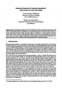
results by creating a collection of computational negative controls from the original dataset. Specifically, we generate a collection of m randomized datasets from our original dataset, in which independent random permutations are applied to the individual components of the attribute vector associated with each object. We then cluster both the original dataset and the m randomizations using the same clustering procedure and compare the results. The idea is that large differences between the original results and the randomizations are indicative of significant cluster structure that has been destroyed by the randomization. Applying this procedure then provides a basis for addressing both of the practical questions raised above. Specifically, the difference be1 Introduction tween the original and randomized results provides the There is considerable interest in the use of unsupervised basis for a quantitative assessment of the significance clustering methods to discover structure in datasets of the clustering results obtained, and these significance [4, 5, 9, 11, 12, 15], with much recent interest in results can then be used together with cluster quality clustering gene expression data [2, 6, 8]. Partition-based results to decide how many clusters are present in the clustering methods will generally partition any dataset dataset when there is evidence in support of a cluster D into a specified number of disjoint subsets, regardless structure. The following example provides a simple ilof how appropriate such a partitioning may be to the lustration of this basic procedure, and subsequent secdataset. As a practical consequence, the following two tions of the paper consider various aspects of the proquestions are both important and difficult to answer: cedure in more detail. A. Does the dataset under consideration actually ex2 Illustrative example hibit a natural cluster structure? The example considered here is based on the Ruspini B. If so, how many clusters k are present in the dataset [15], consisting of 75 bivariate attribute vectors. dataset? This dataset was chosen because it represents a simple, well-known example that is commonly used as a benchIn biology, negative controls are commonly used to asmark problem in evaluating clustering methods and is sess the effects of an experimental treatment: samples widely available, incorporated as a built-in data object that are known a priori not to respond to the treatin both the R and S-plus statistics packages. The left ment provide a basis for deciding how “significant” the hand plot in Fig. 1 is a scatterplot of these attribute vecobserved responses are for the other samples. Here, we tors, which shows the existence of four reasonably wellapply this idea to assessing the significance of clustering defined clusters, although some have argued in favor of a five cluster description [5]. The right-hand plot in Fig. ∗ The authors wish to acknowledge support for this work 1 shows the results of applying a random permutation from the National Institutes of General Medical Sciences and to the second component of the attribute vector, largely Mental Health (MH64459-01) and the Defense Advanced Research destroying this cluster structure. The consequences of Program Administration BioSpice initiative (F30602-01-0578). † Daniel Baugh Institute for Functional Genomics and Compusuch permutations are discussed in detail in Sec. 2.3, tational Biology, Thomas Jefferson University, Philadelphia, PA. using the basic computational negative control (CNC) T. Zylkin is currently with Department of Mathematics, Univer- procedure described next.

Abstract

Most partition-based cluster analysis methods (e.g., kmeans) will partition any dataset D into k subsets, regardless of the inherent appropriateness of such a partitioning. This paper presents a family of permutation-based procedures to determine both the number of clusters k best supported by the available data and the weight of evidence in support of this clustering. These procedures use one of 37 cluster quality measures to assess the influence of structure-destroying random permutations applied to the original dataset. Results are presented for a collection of simulated datasets for which the correct cluster structure is known unambiguously.

sity of Pennsylvania.

150 100

3. Generate answers to Questions A and B above: A. If min{pk } < θ where θ is a specified significance threshold, the dataset D exhibits evidence of significant structure.

50

y value

B. If significant structure is detected, select the “best” choice of k from these results.

0

0

50

y value

150

Permutation of y values

100

Original Ruspini dataset

0

20

40

60

80

100

120

0

20

x value

40

60

80

100

120

x value

Figure 1: Plots of the original Ruspini dataset (left-hand side) and the result of a random permutation applied to the y variable (right-hand side) 2.1 Computational procedure The basic CNC procedure proposed here consists of the following steps: 0. Formulation: specify a dataset D, the maximum number k ∗ of clusters to consider, a clustering method M, a cluster quality measure Q(·), and a number m of negative control datasets to generate. 1. For each k = 2, 3, . . . , k ∗ , do: a. Obtain the k-cluster partition P0k of the dataset D using method M. b. Compute the quality measure Q(P0k ) for this clustering result. c. For each i in 1 to m, do: i. Generate a new structure-destroying permutation πi D of the dataset D. ii. Obtain the k-cluster partition Pik of the dataset πi D using method M. iii. Compute the quality measure Q(Pik ) for this clustering result. 2. Develop and examine both graphical and numerical summaries of the results: a. Generate side-by-side boxplot summaries of the m Q(Pik ) values for k = 2, 3, . . . , k ∗ . b. Plot the values of Q(P0k ) for k = 2, 3, . . . , k ∗ on the same plot with the boxplots generated in (a). Note that if significant cluster structure in the original dataset has been destroyed by the random permutations, some of the values of Q(P0k ) should fall well outside the range of variation seen in the Q(Pik ) boxplots. c. Compute p-values pk for the null hypothesis that Q(P0k ) has the same distribution as the permutation results {Q(Pik )}.

This paper investigates the 37 cluster quality measures Q(·) described by Bolshakova and Azuaje [2], who used them with random subset selection to assess cluster stability (i.e., the degree to which “similar” datasets gave “similar” clustering results). Here, our objective is the opposite: we wish to destroy the structure present in the original dataset and look for large changes in the result, indicative of significant cluster structure in the original dataset. Because we consider so many different quality measures, this paper restricts consideration to a single clustering method M, the Partitioning Around Medoids (PAM) procedure described by Kaufman and Rousseeuw [12], with the popular Euclidean dissimilarity measure. This procedure was chosen because it is available in both the R and S-plus software packages, it has been described in reasonable detail [12], and it overcomes a number of the known limitations of the more popular k-means clustering procedure (e.g., its outlier sensitivity and its dependence on the original ordering of the objects in the dataset). Clearly, the quality of the results obtained here can depend strongly on the method M chosen, and follow-on studies are planned to examine this influence in detail. Indeed, one of our motivations for undertaking this work is to provide a practical, data-based platform for comparing the performance of different clustering algorithms. 2.2 Silhouette coefficients One of the 37 cluster quality measures considered here is the silhouette coefficient [11, 12], based on the idea that a “good” clustering should consist of well-separated, cohesive clusters, and defined as follows. Given a partitioning P of a set of N objects into k clusters, consider any fixed object i and let Ci denote the set of indices for all objects clustered together with object i. As a cohesion measure for cluster Ci , take the average dissimilarity between object i and all other objects in Ci : a(i) =

1 X dij , ni j∈Ci

where dij is the dissimilarity between objects i and j and ni is the number of objects in cluster Ci . To characterize the separation between clusters, let K` denote the `th neighboring cluster, distinct from Ci , for ` = 1, 2, . . . , k − 1. Define b(i) as the average

s(i) =

b(i) − a(i) . max{a(i), b(i)}

For the silhouette coefficient s(i) to be well-defined, P must contain at least two clusters and every cluster in P must contain at least two objects. Then, it is not difficult to show that the silhouette coefficient satisfies −1 ≤ s(i) ≤ 1 for all i and these limits have the following interpretations. If cluster Ci is “tight,” all of its objects exhibit small dissimilarities, implying that a(i) is a small positive number. Similarly, if cluster Ci is well-separated from all of its neighbors, b(i) is a much larger positive number so max{a(i), b(i)} = b(i) and b(i) − a(i) ' b(i). Hence, for an object i in a tight cluster, well separated from its neighbors, s(i) ' 1. Conversely, suppose object i has been assigned to the wrong cluster by a clustering procedure. It then follows that a(i) is a large positive number (reflecting its dissimilarity to the other objects it is clustered with) and b(i) is a small positive number (i.e., its “nearest neighbor cluster” is really the cluster it belongs in). In this case, max{a(i), b(i)} = a(i) and b(i)−a(i) ' −a(i), implying s(i) ' −1. Finally, if there is little or no inherent cluster structure, we would expect that a(i) and b(i) would be about the same (i.e., the “best cluster” for object i is essentially no better than the “second best cluster” for that object), implying s(i) ' 0. A useful overall quality measure for a given clustering is its average silhouette coefficient: s¯ =

N 1 X s(i). N i=1

Based on their experience, Kaufman and Rousseeuw [12, p. 88] offer the following suggestions for the interpretation of s¯ as a measure of evidence in support of cluster structure: - 0.70 < s¯ ≤ 1.00 ⇒ strong evidence - 0.50 < s¯ ≤ 0.70 ⇒ reasonable evidence - 0.25 < s¯ ≤ 0.50 ⇒ weak evidence - s¯ ≤ 0.25 ⇒ no significant evidence.

0.8 0.7 0.6 0.5 0.4

The silhouette coefficient s(i) for object i is defined as the normalized difference:

0.3

j∈K`

0.2

dissimilarity between object i in cluster Ci and the objects in the closest neighboring cluster, i.e.    1 X b(i) = min dij .  `  n`

k=2

k=3

k=4

k=5

k=6

k=7

k=8

Figure 2: Boxplot summaries of the permutation-based average silhouette coefficient values, plotted against the number of clusters k The advantage of the permutation results presented here is that they give additional support to these conclusions when they are valid, offering the possibility of attaching statistical significance to these statements. In particular, note that if the value of s¯ computed from the original dataset is larger than all but q − 1 of the m permutation values, the (one-sided) probability of observing a value this extreme in the permutation data is less than q/m. As a consequence, we can take the observation of such average silhouette coefficient values as evidence that structure in the original dataset has been destroyed at a significance level of q/m. This additional information is especially useful in cases where the silhouette coefficients are either somewhat marginal (e.g., less than 0.5) or misleading by themselves, a problem discussed further in Sec. 6. 2.3 Results and significance Fig. 2 shows a boxplot summary of the average silhouette coefficient values s¯ obtained after applying the PAM clustering procedure to each of 200 random permutations of the Ruspini dataset (specifically, these permutations were applied to the second component of each attribute vector; the first component was not modified). In addition, the average silhouette coefficient values computed from the original dataset are shown as solid circles in this plot, and the horizontal dashed lines represent the interpretation threshold values discussed above. Here, the clustering results for k = 2 through k = 6 all clearly support the structure hypothesis at the 0.5% level, since they all exceed the corresponding 200 permutation values. Taking the maximum of these significant s¯ values as the most likely number of clusters present gives the correct result, k = 4. Also, note that the evidence in support of the secondary choice k = 5 appears almost as strong as that for k = 4, lending credence to the argument for

• -3

-2

-1

0

1

2

0.46 0.42

• ••• •••• •• •••••••• •••••• ••••••• • • • • • • • • • ••••••••• •••••••• •••••••• ••••••••••••• ••••••••••••••••• ••••

0.38

•

0.34

0.51 0.49

••

Permutation Silhouette Value

Clusters: k = 4 •

0.47

Permutation Silhouette Value

Clusters: k = 2

3

• •

•• • • •• •••• •••••• ••••••• •••••••• •••••• • • • • • ••••• ••••••• •••••••• •••••••• ••••• •••••••• •••••••• • • • • • • •••• • ••

-3

-2

Quantiles of Standard Normal

-3

-1

0

1

1

2

2

Quantiles of Standard Normal

3

0.44

0.48

•• • •••• ••• ••• •••••••••• ••••••••• ••••••••• • • • • • ••••••• ••••••• •••••• ••••••• ••••••••• •••••• ••••••••• • • • •••

0.40

Permutation Silhouette Value

• •

• -2

0

3

Clusters: k = 8

• ••• ••••• ••••••••• •••••• •••••••••• •••••• • • • • ••••••• •••••••• ••••••• •••••••• •••••• •••••••••••• ••••••

•

• • •

0.36

0.50 0.45 0.40

•

0.35

Permutation Silhouette Value

Clusters: k = 6

•

-1

Quantiles of Standard Normal

-3

-2

-1

0

1

2

3

s¯

z

2 3 4 5 6 7 8

0.58 0.63 0.74 0.71 0.60 0.49 0.45

11.66 6.47 13.60 10.20 6.48 2.55 0.71

p

0 5 × 10−11 0 0 5 × 10−11 0.005 0.239

Quantiles of Standard Normal

Figure 3: Normal Q-Q plots for the k cluster permutation results, k = 2, 4, 6, and 8. this secondary choice. Support for other choices of k is substantially weaker, both in terms of the average silhouette values themselves and in terms of the distance these values lie from the 200 permutation results. This last observation raises an important point. The arguments just presented do not depend on the distribution of the permutation values, only on the hypothesis that all permutations are equivalent (specifically, that the randomized datasets are exchangeable [10]). As a consequence, in the practically important case where the original result falls outside the range of the permutation results, strictly rank-based interpretations make no use of the distance between the original and the randomized results. Frequently, however, the randomized results exhibit an approximately normal distribution, permitting us to make stronger statements about significance that do account for this distance. Specifically, define the z score for each set of results as: z=

k

s¯0 − s¯p , σ

where s¯0 is the value of s¯ computed from the original dataset, s¯p is the average of the m permutation values for s¯, and σ is the standard deviation of these m permutation s¯ values. Under the approximate normality assumption just described, the probability of observing a value of z larger than Z is 1 − Φ(Z) where Φ(x) is the standard Gaussian cumulative distribution function. The normal quantile-quantile (Q-Q) plot provides a useful informal test of the approximate normality hypothesis for a given dataset [3]. This plot shows the rank-ordered data values, sorted from smallest to largest, as a function of the rank order: if the approximate normality assumption is reasonable, this plot should appear as a straight line. D’Agostino and Stephens [3] argue against using Q-Q plots for datasets smaller than about 50 numbers, but these plots are quite

Table 1: Summary of silhouette coefficieint permutation results for the Ruspini dataset

useful for characterizing the 200 permutation results considered here. Fig. 3 shows normal Q-Q plots for these results for k = 2, 4, 6, and 8, from which it is clear that the approximate normality assumption is reasonable here. Consequently, the Gaussian pvalues are computed and listed in the last column of Table 1. The extreme significance of these p values greatly strengthens the permutation-based conclusions presented above. Finally, note that even if normality is not a reasonable approximation, so long as the permutation results exhibit a unimodal distribution, the probability of observing a particular result in the randomized data decreases monotonically (and usually rapidly) with increasing z scores. Hence, even under this much weaker distributional assumption, larger z scores can be taken as stronger evidence in support of a particular cluster structure hypothesis. 3 Other quality measures In addition to the silhouette coefficients defined in Sec. 2.2, we also consider the 36 cluster validity measures introduced by Bolshakova and Azuaje [2], representing 18 variations of each of the cluster validity measures proposed by Dunn [9] and Davies and Bouldin [4]. 3.1 Dunn’s index The index proposed by Dunn [9] is based on a partitioning P of the dataset D into k clusters Ci , i = 1, 2, . . . , k, a distance measure (intercluster distance) δ(Ci , Cj ) between distinct clusters, and a cohesion measure (intracluster distance) ∆(Ci ) for each cluster. These distances may be computed in various ways, discussed further in Sec. 3.3, but here it is enough to note that both of these quantities are assumed to be positive for all clusters. Given these quantitites, Dunn’s

metric for the quality of a clustering is given by:    δ(Ci , Cj ) Q(P) = min min i j6=i max` {∆(C` )} mini {minj6=i {δ(Ci , Cj )}} = . max` {∆(C` )} Note that if all clusters are well-separated with respect to the intercluster distance measure δ(·, ·) and “tight” with respect to the intracluster distance measure ∆(·), Dunn’s index will assume a large positive value. Hence, one approach to selecting the number of partitions k in a dataset is to maximize Q(P) with respect to k. Like the silhouette coefficients s(i), Dunn’s metric is not applicable to unclustered datasets: it is not computable for the case k = 1.

The complete linkage distance δ2 (S, T ) is the distance between the two most distant objects in the two clusters, defined by: δ2 (S, T ) = max dij . i∈S,j∈T

The average linkage distance δ3 (S, T ) is the average distance between objects in the two clusters, given by: δ3 (S, T ) =

1 |S||T |

X

dij .

i∈S,j∈T

Note that all three of these intercluster distance measures are closely related to hierarchical clustering procedures [12], and they are computable from the object dissimilarity matrix alone. The next two intercluster distance measures require knowledge of the distance function itself, since they involve the centroids cs and ct of the clusters S and T , whose j th components are defined by:

3.2 The Davies-Bouldin index The index of Davies and Bouldin [4] represents a different combination of the same elements used to define Dunn’s index. Specifically, given a clustering P and the quantities 1 X i 1 X i x , [c ] = xj , [c ] = t j s j j δ(Ci , Cj ) and ∆(Ci ) defined in Sec. 3.1, the Davies|S| |T | i∈S i∈T Bouldin index is defined as   k where xij is the j th component of the attribute vector xi 1 X ∆(Ci ) + ∆(Cj ) (3.1) Q(P) = max . for object i. Note that the centroids are generally not k i=1 j6=i δ(Ci , Cj ) objects in the original dataset, so complete knowledge In contrast to Dunn’s index, the Davies-Bouldin index of the original dissimilarity matrix is not sufficient should exhibit small values for well-separated, compact to compute either the centroids or the following two clusters. Hence, the optimum number of clusters in a intercluster distance measures. Denoting the distance dataset may be determined by minimizing Q(P) with function between attribute vectors x and y by d(x, y), respect to k. Also, like Dunn’s index, the Davies- the centroid linkage distance δ4 (S, T ) is given by: Bouldin index is not defined for the unclustered case, δ4 (S, T ) = d(cs , ct ), k = 1. Finally, as a practical matter, we have found plots of the logarithm of the Davies-Bouldin index to be more useful than plots of the raw index values. Hence, and the average to centroids linkage distance δ5 (S, T ) is in the following discussions, the term “Davies-Bouldin given by: ! index” will refer to the logarithm of the expression X X 1 i i defined in Eq. (3.1). d(x , ct ) + d(x , cs ) . δ5 (S, T ) = |S| + |T | i∈S

3.3 The Bolshakova-Azuaje family Evaluation of either of the cluster quality indices just described requires computable definitions of the intercluster distance δ(Ci , Cj ) between two distinct clusters Ci and Cj and the intracluster distance ∆(Ci ) for every individual cluster Ci . The following paragraphs describe the six choices of δ(Ci , Cj ) and the three choices of ∆(Ci ) proposed by Bolshakova and Azuaje [2] in their study of cluster stability. Let S and T be two different clusters, of size |S| and |T |. The single linkage distance δ1 (S, T ) is the closest distance between objects belonging to the distinct clusters S and T , given by: δ1 (S, T ) =

min

i∈S,j∈T

dij .

i∈T

Finally, the Hausdorff distance δ6 (S, T ) is defined as: δ6 (S, T )

= max{h(S, T ), h(T , S)}

h(X , Y)

= max {min{dij }}. i∈X

j∈Y

The three intracluster distances proposed by Bolshakova and Azuaje [2] are the complete diameter, defined as ∆1 (S) = max {dij }, i,j∈S

the average diameter, defined as ∆2 (S) =

1 |S|(|S| − 1)

X

i,j∈S,j6=i

dij ,

p

k

Description

10 2 10 3 3 10 10

1 3 4 4 2 2 2

Uniform on the unit cube in R10 Well-separated Gaussian clusters 3 informative, 7 noise components Informative part of Model 3 Two elongated clusters Model 5 plus 7 noise components Overlapping, 9 noise components

and the centroid diameter, defined as ∆3 (S) =

2 X d(xi , cs ). |S|

1.0

3

4

5

6

7

8

Figure 4: Permutation results for the Ruspini dataset with the Dunn(2,1) index

40

Table 2: Summary of the Dudoit and Fridlyand models and variations considered here

2

30

1 2 3 30 5 6 7

1.5

2.0

Model

4

Case study

The following paragraphs present partial results from a case study based on the Ruspini dataset and a variant of the eight simulation-based datasets described by Dudoit and Fridyland [8]. These models are summarized in Table 2 and they include a uniformly distributed random dataset (Model 1) that has been advocated as a structureless null model for cluster validation [11, p. 186], three models with clear structure like the Ruspini dataset (Models 2, 30 , and 5), extensions of two of these three models obtained by adding spurious noise components to the attribute vectors (Models 3 and 6), and a model with two overlapping one-dimensional clusters and nine spurious noise components (Model 7). Fig. 4 shows the results obtained for the Ruspini dataset using the Dunn index based on the complete linkage intercluster distance δ2 (S, T ) and the complete diameter ∆1 (S). The boxplots in this figure summarize 50 random permutations of the dataset, giving one-sided significance values of p = 0.02 whenever the Dunn index computed from the original dataset exceeds all of the permutation values. Here, the only significant result is that for k = 4, which corresponds to the correct cluster structure. For comparison, Fig. 5 shows the results obtained using the average to centroids distance δ5 (S, T ) with ∆1 (S), which exhibit significant results

10

Note that like the intercluster distances δ4 (S, T ) and δ5 (S, T ), the centroid diameter ∆3 (S) requires knowledge of the dissimilarity function d(·, ·) and not just the pairwise dissimilarity matrix between the objects in the original dataset.

20

i∈S

2

3

4

5

6

7

8

Figure 5: Permutation results for the Ruspini dataset with the Dunn(5,1) index

for both k = 2 and k = 4. In fact, both the Dunn index values (Q(P) ' 36 vs. 25) and their associated z values (10.51 vs. 7.93) strongly favors k = 2 over the correct value k = 4. This result is considered further at the end of this section, but the key point is that the choice of the 18 options considered here for defining Dunn indices is quite important in practice. Results obtained for the Ruspini dataset using the Davies-Bouldin indices with the same choices of intercluster and intracluster distances as in the first example are shown in Fig. 6. Recall that for the DaviesBouldin index, small values are better than larger ones, so we are interested in those values of k for which the Davies-Bouldin index values computed from the original dataset lie below the smallest of the permutation values. Here, we have two such values: k = 4 and k = 5, in agreement with the results obtained from the silhouette coefficients. Both the fact that the Davies-Bouldin index value is smaller for k = 4 than for k = 5 and the fact that the z value is more negative for k = 4 than for k = 5 support the generally preferred interpretation of the Ruspini dataset as containing four clusters.

0.9

0.6

0.8

0.4

0.6

0.7

0.2

0.5

0.0

0.4

−0.2

2

3

4

5

6

7

8

0.50

0.55

0.60

0.65

0.70

0.75

0.80

Figure 6: Permutation results for the Ruspini dataset with the DB(2,1) index

2

3

4

5

6

7

8

Figure 7: Permutation results for the Model 1 dataset with the DB(2,1) index

Results obtained from Model 1 with the DB(2,1) index are shown in Fig. 7. Here, as in all other cases involving attribute vectors of dimension p > 2, independent random permutations are applied to all but the first of the p components of this vector. In this particular example, no cluster structure is present, so none of the original cluster quality indices should be significant relative to the permutation results, and this is precisely the result seen in Fig. 7 for k = 2 through k = 8. In contrast, Fig. 8 shows the results obtained for this structureless dataset from the Davies-Bouldin index based on the same intercluster distance (complete linkage, δ2 (S, T )) but with the centroid diameter ∆3 (S) instead of the complete diameter, ∆1 (S). There, significant evidence appears in support of any number of clusters between k = 3 and k = 8, with strongest support for k = 7, which has both the smallest Davies-Bouldin index value and the most negative z score. More generally, the behavior seen in Fig. 8 is characteristic of the results obtained using the centroid diameter ∆3 (S) with any choice of intercluster distance, for either the Dunn indices or the Davies-Bouldin in-

2

3

4

5

6

7

8

Figure 8: Permutation results for the Model 1 dataset with the DB(2,3) index

dices. That is, results based on ∆3 (S) almost always give high significance to a wide range of k values, frequently with a shallow maximum (for the Dunn indices) or minimum (for the Davies-Bouldin indices) at a fairly large value of k. Further, of the 37 cluster quality measures considered here, only those based on the centroid diameter provided evidence for cluster structure in the structureless Model 1 dataset. Similarly, the average to centroids intercluster distance δ5 (S, T ) also appears to perform badly for many of the examples considered here. For example, this intercluster distance was the only one that gave strong support for the incorrect number of clusters in the Ruspini dataset, as seen in Fig. 5. Further, δ5 (S, T ) was the only intercluster distance that led to incorrect clustering results for Model 30 using the Dunn indices. Also, the results obtained for the Davies-Bouldin indices were consistently incorrect for this model whenever they were based on δ5 (S, T ). Comparing the Dunn and Davies-Bouldin indices across all of the datasets considered here, it appears that the Dunn indices generally yield better results. For example, the Dunn index based on the centroid linkage distance δ4 (S, T ) and the complete diameter ∆1 (S) found no structure in the structureless Model 1 dataset, but the Davies-Bouldin index based on the same pair of distances gave clear support for k = 5 clusters. More dramatic differences are seen for Model 3, where 7 of the 18 Dunn indices gave reasonably clear evidence for the correct cluster structure (k = 4), but none of the Davies-Bouldin indices gave clear support for this structure. 5

Extraneous attributes

This last result illustrates an important point: Models 3, 6, and 7 are difficult to cluster correctly, due to the presence of many extraneous noise components.

Noise Components

s¯, k=2

s¯, k=4

z, k=2

z, k=4

0 1 2 3 4 5 6 7

0.636 0.619 0.604 0.587 0.579 0.568 0.557 0.548

0.750 0.709 0.675 0.638 0.619 0.595 0.573 0.555

70.38 52.88 49.12 28.51 23.53 23.49 22.15 23.02

22.89 19.51 20.99 25.29 17.44 23.92 17.47 18.82

Table 3: Average silhouette coefficients and z values for k = 2 and k = 4 as a function of the number of noise components included in Model 3

This point has been noted previously [11, p. 24] as an argument against including possibly extraneous attributes in cluster analysis. Our results strongly support this cautionary argument. For example, results obtained for Model 30 give clear evidence for the correct number of clusters for 14 of the 18 Dunn indices considered here, but we only obtain comparably clear evidence for the correct clustering for 7 of the 18 Dunn indices for the Model 3 data, which includes the three informative attributes from Model 30 and seven unrelated noise components. This difference is even more pronounced for Models 5 and 6, which also differ by the presence of seven unrelated noise components. There, both the Dunn and the DaviesBouldin indices give the correct results in all 18 cases for Model 5, but only two of the Dunn indices and one of the Davies-Bouldin indices find the correct structure for Model 6. The results for Model 7, which has overlapping univariate clusters and nine unrelated noise components, are even worse: none of the 37 cluster quality measures considered here gives clear evidence for the correct structure. Table 3 shows how the results obtained for Model 30 with the silhouette coefficient degrade as additional noise components are included in the attribute vectors used for clustering. In the absence of any extraneous noise components (i.e., for Model 30 ), the average silhouette value for k = 4, the correct result, is significantly larger than that for k = 2, the case with the second-largest s¯ value. As noise components are added, two things happen. First, the average silhouette coefficient values all decrease in magnitude, suggesting poorer clustering, although they all remain highly significant relative to the permutation results, based on the very

large z values listed in Table 3. Second, the difference between the average silhouette coefficient for k = 4 and that for k = 2 decreases monotonically as more noise components are included in the attribute vectors. In particular, note that by the time seven noise components have been included (i.e., for Model 3), these average silhouette coefficients only differ by about 1%. 6 Overall assessment The general CNC strategy described here starts with a set {Pk } of k-partition clusterings for a given dataset over a specified range of k values. Using structuredestroying permutations, we then assess the significance of the cluster structure found for each k with some measure of cluster quality, Q(Pk ). Finally, we retain only those partitionings Pk that show significance, either in terms of permutation statistics alone (i.e., the rank of the original data clustering relative to the m permutations) or using z scores as a more quantitative measure of significance. The best of these significant partitionings with respect to the quality measure Q(·) is then taken as the partitioning Pk∗ best supported by the data. In favorable cases, the clustering that maximizes the quality measure Q(·) will also exhibit the most significant z score, and this z score will be far larger than all of the others. This behavior is nicely illustrated by the Dunn(3,1) index results obtained for Model 30 . There, the correct clustering (k = 4) exhibits both the largest Q value (1.41) and the most significant z score (20.73); in contrast, the second-best result is obtained for k = 2, with a Q value of 1.05 and a z score of 8.78, and the third-best result is that for k = 3, with a Q value of 0.74 and a z score of 5.41. Also, these Q values are the only three that fall outside the range of the 50 randomizations considered for this example. Hence, in this case, both the z score and the Q value argue in favor of the correct result, k = 4. Conversely, it frequently happens that the partitioning that maximizes the quality measure Q(·) is not significant and indeed, corresponds to the incorrect partitioning. A specific example where this occurs is the result obtained for the Dunn(2,3) index computed from Model 3. There, the largest Q value is 2.15, obtained for k = 2, but this Q value falls within the range of the randomized Q values, with a z score of only 0.91. In contrast, the largest significant Q value is 1.98 for the correct structure, k = 4, falling well outside the range of randomized Q values, with a z score of 7.36. It is also important to note that maximizing the z score does not give the correct partitioning in this case: the maximum z score seen in this example is 10.89, obtained for k = 8, but the Q value for this case is only 1.20. In general, we have found that the combined use of both Q values

for the original dataset and their associated z scores as described here gives better results than the use of either Q values or z scores alone. Overall, the results obtained for the datasets considered here demonstrate that the proposed CNC approach to cluster validation is extremely effective in favorable cases. In particular, all of the 37 cluster quality measures we examined gave the correct results for the Model 5 dataset, and most gave the correct results for the Ruspini and Models 1, 2, and 30 datasets. Conversely, we have also seen that this approach fails in difficult cases like those containing many spurious noise components: we never obtained the correct results for Model 7, rarely for Model 6, and only occasionally for Model 3. Part of this difficulty may lie in the clustering algorithm used here (procedure PAM with Euclidean dissimilarities), although clustering is known to be difficult under these circumstances, as discussed in Sec. 5. We are exploring the question of method dependence further and will report the results elsewhere. In general, our results suggest that silhouette coefficients represent the best of the 37 cluster quality measures considered here. Specifically, silhouette coefficients gave clear, correct results for the Ruspini dataset and for Models 1, 2, 30 , and 5. Further, silhouette coefficients gave marginally correct results for Model 6, for which almost none of the other 36 quality measures gave correct results. The poorest relative performance for the silhouette coefficients was obtained for Model 3, for which the results were very marginal and clearly inferior to those obtained with three of the Dunn indices (specifically, Dunn(1,1), Dunn(3,1) and Dunn(6,2)). As noted, none of the 37 measures considered here gave correct results for Model 7. In addition to their generally superior performance relative to the other cluster quality measures considered here, the silhouette coefficients also have the advantage of normalization, lying in the range −1 ≤ s¯ ≤ 1 and having the informal interpretation guidelines presented in Sec. 2.2. In contrast, the other 36 cluster quality measures considered here are only constrained to be positive and the observed ranges of variation depend strongly both on the choices of δ(S, T ) and ∆(S) and on the datasets considered. Conversely, the results just noted also indicate that silhouette coefficients do sometimes fail to give the correct result in situations where some of the other cluster quality measures considered here can give the correct result. This observation motivates our continued interest in these alternatives, although it does appear that the list of 36 choices considered here can be pared down substantially. First, almost without exception in the examples considered here, the Dunn index based on any given combination of intercluster and intraclus-

i, j

k ∗ , 30

Q, 30

z, 30

k∗ , 3

1,1 1,2 1,3 2,1 2,2 2,3 3,1 3,2 3,3 4,1 4,2 4,3 5,1 5,2 5,3 6,1 6,2 6,3

4 4 4 4 4 4 4 4 4 4 4 4 2 2 2∗ 4† 4 4

0.70 1.68 1.18 2.10 5.00 3.51 1.41 3.34 2.35 1.36 3.24 2.27 73.40 156.85 102.13 1.45 3.46 2.42

28.95 27.26 47.51 14.49 15.35 21.07 20.73 23.96 28.24 26.35 32.00 36.29 10.04 18.03 2.50 10.68 11.33 18.14

4 4† 4 2 2∗ 4 4 2† 4 4† 2 2† 2 2 2 2∗ 4 4

Q, 3

z, 3

0.65 1.15 0.83 1.64 3.15 1.98 1.10 1.95 1.39 0.96 1.79 1.23 70.09 134.24 91.67 1.33 2.07 1.48

20.79 17.04 24.88 4.90 3.04 7.36 12.82 10.34 11.97 16.89 18.23 5.74 8.12 11.55 3.45 2.29 3.83 7.25

Table 4: Summary of the 18 Dunn(i,j) index results for Models 30 and 3

ter distances gave better results than the corresponding Davies-Bouldin index. Also, it was noted that both Dunn and Davies-Bouldin indices based on the centroid diameter ∆3 (S) often gave poor results, as did these indices based on the average to centroids linkage distance, δ5 (S, T ). This point is illustrated clearly in Table 4, which summarizes the results obtained for all 18 of the Dunn indices considered here, for Models 30 and 3. Specifically, this table lists the number of clusters k ∗ identified in the dataset, the associated quality measure Q = Q(Pk∗ ), and the associated z-score. Entries where k ∗ is marked with the symbol † represent ambiguous cases where the difference in Q values between the best and second-best k values were quite small. Note that all three of the Dunn(5,j) indices gave the incorrect results for Model 30 , and these were the only cases where the Dunn indices failed to identify the correct structure, as noted in Sec. 4. Conversely, note that in this case if we had chosen k to maximize the z score, we would have obtained the correct result. This situation also occurs twice for Model 3, for the Dunn(2,2) and Dunn(6,1) indices; these cases are marked with ∗ in Table 4. Also, as in the results presented in Sec. 5 for the silhouette coefficients, the degradation caused by the addition of unrelated noise components is clear for the Dunn indices as well. In particular, note that the Q

values obtained for Model 3, containing the 7 extraneous noise attributes, are always smaller than those for Model 30 , which contains only the 3 information-bearing attributes from Model 3. Similarly, in every case except Dunn(5,3), the z scores for the predicted clustering are smaller for Model 3 than for Model 30 . Conversely, it is also clear that the extent of this degradation is a strong function of the specific Dunn index considered. For example, it may be seen in Table 4 that the differences between the results for Model 30 and Model 3 are fairly minor for Dunn(1,1): the Q value is about 7% smaller for Model 3, the z score is about 28% smaller but still quite significant, and the correct number of clusters is identified in both cases. In contrast, the differences are much more pronounced for Dunn(2,2): the Q value declines by 37%, the z score declines by 80%, and the correct number of clusters is not identified for Model 3.

through k = kmax and, from these, the corresponding set of quality measures {Q(Pkr )}. Since Q(P) > Q(P 0 ) implies partitioning P is better than partitioning P 0 here, useful insights may be obtained by looking at the following differences: (7.2)

δk = Q(Pk ) − Q(Pkr ).

In particular, note that if δk is a large positive number, this result provides preliminary evidence in support of k significaant clusters. To determine what is “large,” it may be desirable to consider a normalized quantity like (7.3)

∆k =

Q(Pk ) − Q(Pkr ) , Q(Pk ) + Q(Pk )r

which satisfies |∆k | ≤ 1 for Dunn’s index or other inherently positive cluster quality measures. Conversely, for normalized measures like the silhouette coefficient, it is enough to examine δk directly since |Q(P)| ≤ 1 im7 Computational considerations plies |δk | ≤ 2. In any case, preliminary evaluation of δk The results presented in this paper were obtained using or ∆k values provides a basis for excluding values of k the basic CNC procedure outlined in Sec. 2.1, but sevfor which significant evidence of cluster structure in the eral reviewers raised concerns over the computational dataset appears unlikely. complexity, which is m + 1 times that of standard clusThis idea extends directly to comparison of other tering method M on which it is based. We acknowledge clustering characteristics besides the number of clusthe importance of this concern and we are exploring sevters k. In particular, the same strategy could be used eral approaches to reduce this basic complexity. The folto compare different clustering methods {Mi }, differlowing discussions briefly outline two preliminary ideas ent dissimilarity measures, or any other method- or that are clearly useful in special cases and which may pretreatment-related computational options that might be useful in developing more general approaches. be of interest. The practical value of this idea lies in the fact that we can exclude analysis options that are 7.1 Exploratory comparisons Although it does unlikely to characterize whatever structure is present in not provide the basis for computing statistical signifithe dataset at twice the standard clustering cost, rather cance levels, applying the general procedure described than m + 1 times this cost for some large m. here with a single randomization (i.e., with m = 1) does provide comparisons that may be extremely useful in 7.2 Separable dissimilarities A significant contrian exploratory analysis context. In what follows, we bution to the computational cost of clustering using gensuppose Q(·) is a cluster quality measure like Dunn’s eral procedures like the PAM algorithm employed here index or the silhouette coefficient, for which larger valis the expense of forming the N × N dissimilarity maues correspond to better clustering results, although trix D, given a set of N attribute vectors of dimension the idea extends immediately to indices like the Daviesp. In fact, since dissimilarities satisfy dii = 0 for all Bouldin index for which smaller values corresond to beti and dji = dij for all i and j [11, 12], it is enough to ter clustering results. Given a dataset D and a range compute the N (N −1)/2 elements of this matrix, dij for kmin ≤ k ≤ kmax of candidate cluster numbers, first i > j. If the cost of computing each element dij is C, partition the unmodified dataset D for this range of k the total cost associated with the basic CNC procedure values using any method M to obtain the collection described here is approximately mN 2 C/2. This com{Pk } of clusterings for k = kmin through k = kmax . putational cost may be traded for storage space if we From these results, compute the corresponding qualconsider separable dissimilarity measures of the general ity measures {Q(Pk )}. Next, apply independent ranform: p dom permutations to components 2 through p of the X p-component attribute vector associated with each ob- (7.4) dij = δ(i, j, `), ject to obtain a single randomized dataset D r . Apply `=1 clustering method M to this new dataset to obtain the where δ(i, j, `) is the contribution of component ` of the corresponding set of partitionings {Pkr } for k = kmin attribute vectors xi and xj to the total dissimilarity.

The best known separable dissimilarity measure is the Manhattan (L1 ) distance, for which (7.5)

δ(i, j, `) = |x`i − x`j |.

numbers, x and y, their Pythagorean sum is defined as p x ⊕ y = x2 + y 2 , (7.8)

and Moler and Morrison describe a procedure for comAlso, note that while the Euclidean (L2 ) dissimilarity puting x ⊕ y directly from x and y, without either formis not of this form, the squared Euclidean distance is ing squares or taking square roots. In the context of separable, corresponding to the problem considered here, note that the Eudlidean distance dij between attribute vectors xi and xj is (7.6) δij` = |x`i − x`j |2 , (7.9) dij = δ(i, j, 1) ⊕ δ(i, j, 2) ⊕ · · · ⊕ δ(i, j, p), an observation that leads to some possible extensions, discussed at the end of this section. where δ(i, j, `) is the distance component defined in Now, suppose dij is a separable dissimilarity of the Eq. (7.5) for the Manhattan dissimilarity. Hence, form (7.4) and consider the dissimilarity drij between although Euclidean dissimilarities are not separable the randomized attribute vectors xri and xrj . Note that with respect to ordinary addition, they are separable the effect of the randomization r on the ` component of with respect to Pythagorean addition. In fact, this the original attribute vector xi is to replace x`i with idea could be extended to other dissimilarity measures x`π(r,`;i) , where π(r, `; i) is the ith element of the N - besides the Euclidean case by considering dissimilarities element permutation vector π(r, `). Here, r corresponds that are separable with respect to other variants of to a randomization index, taking values from 1 to m, addition. More specifically, Aczel [1] discusses the and ` corresponds to an attribute component index, general class of associative binary operators that share taking values from 1 to p. The reason this permutation many characteristics of ordinary addition and which can depends on both r and ` is that the permutations be represented in the general form applied to each component of the attribute vector are x ◦ y = φ−1 (φ(x) + φ(y)) , assumed independent; otherwise, if the same random (7.10) permutation were applied to all components of the and attribute vector, π would not depend on `, only on where the function φ : R → R is strictly monotonic 2 continuous. Note that the function φ(x) = x satisfies r the randomization r. The dissimilarity dij for the these conditions when restricted to positive arguments x randomized attributes is given by: and this choice yields the Pythagorean sum x ⊕ y. More p generally, any dissimilarity that can be expressed as an X drij = (7.7) δ(π(r, `; i), π(r, `; j), `). associative binary combination of individual component `=1 dissimilarities can be computed from these component The key observation here is that if we initially compute dissimilarities by direct application of Eq. (7.10) as ! and store the N (N − 1)p/2 component dissimilarities p X −1 δ(i, j, `) for 1 ≤ i < j ≤ N and 1 ≤ ` ≤ p that de- (7.11) φ(δ(i, j, `)) . dij = φ fines any separable dissimilarity, we can compute drij `=1 for any randomization r by simply indexing the appropriate components of this array and adding the results. In a very different context, this idea has been used to While this approach is not practical for very large p define a broad class of nonlinear discrete-time dynamic due to increased storage requirements, it represents a models that can exhibit strongly nonlinear qualitative considerable computational savings in cases where it is behavior while still retaining certain characteristics of linear dynamic models [14]. applicable. Finally, note that this same idea is also applicable to Euclidean distances. In particular, if we store the 8 Summary array of component squared Euclidean distances, we can simply apply the result (7.7) to the separable distance measure defined in Eq. (7.6) and take the square root of the resulting distances dij to obtain the elements of the desired Euclidean dissimilarity matrix. In fact, an even better alternative exists, based on the Pythagorean sum algorithm introduced by Moler and Morrison [13] and refined by Dubrulle [7]. Specifically, given two real

This paper has described a detailed permutation-based procedure for detecting the presence of significant cluster structure in a dataset using unsupervised, partitionbased clustering algorithms. The basic idea is to compute a cluster quality measure for a partitioning of the original dataset and compare it with the range of quality measures obtained from a collection of random permutations applied to the dataset to destroy any cluster

structure that may be present. Large differences in these results may be taken as evidence in support of cluster structure, and this idea may be used to determine the most probable number of clusters present in the dataset. To assess the practicality of this idea, we have compared results obtained for the 37 cluster quality measures described by Bolshakova and Azuaje [2], applied to eight datasets: the Ruspini dataset [12, 15], six of the eight simulation datasets considered by Dudoit and Fridyland [8], and a variation on one of these datasets (Model 30 , described in Sec. 4). Based on the results presented in Secs. 4, 5, and 6, it appears reasonable to restrict consideration to the silhouette coefficient and the Dunn indices, and to drop those indices based on the distance measures δ5 (S, T ) and ∆3 (S), reducing the list of alternative cluster quality measures considered from 37 to 11. Also, note that these two omitted distances represent two of the three centroid-based distances, all of which incur additional computational effort in constructing the required centroids. In particular, the other four intercluster distances—single linkage, complete linkage, average linkage and Hausdorff distances—can all be computed directly from the dissimilarity matrix required for clustering algorithms like the PAM procedure considered here. For this reason, we also drop the centroid linkage distance δ4 (S, T ), leaving nine quality measures: the silhouette coefficient and the Dunn(i,j) indices for i = 1, 2, 3, and 6 and j = 1 and 2. Having established the utility of the permutationbased procedure proposed here and narrowing the set of cluster quality measures from 37 to 9, we are currently examining the influence of alternative dissimilarity measures (e.g., Manhattan distances or productmoment correlations) and alternative clustering algorithms (e.g., k-means). In addition, we are applying these results to biological datasets, starting with publically available datasets like those considered by Dudoit and Fridyland [8] and ultimately examining gene expression datasets that are currently being generated in our laboratory. Based on the preliminary results presented here, we expect these ongoing investigations to provide useful guidance in selecting clustering procedures and in evaluating the effectiveness of different microarray normalization and data pretreatment methods. In particular, note that one of the strengths of the computational negative control framework proposed here is that it can be used to assess the dependence of the weight of evidence in support of a final clustering result on changes in any of the data collection or analysis steps that contribute to that final clustering. For example, Warren and Liu [16] compare a range of normalization methods for microarray data analysis, presenting con-

vincing evidence that reported gene expression values (i.e., the attributes on which a gene clustering would be based) can depend strongly on the various method choices and tuning parameter values adopted (e.g., the smoothing bandwidth in the popular lowess nonparametric smoother). Procedures like the computational negative controls method proposed here should be extremely useful in guiding these selections in cases where a desired intermediate or final result is a functionally significant clustering of genes. References [1] J. Aczel, A Short Course on Functional Equations, Reidel, Dordrecht, 1987. [2] N. Bolshakova and F. Azuaje, Cluster validation techniques for genome expression data, Signal Processing, 83 (2003), pp. 825–833. [3] R. D’Agostino and M. Stephens, Goodness-of-fit Techniques, Marcel Dekker, New York, 1986. [4] D. Davies and D. Bouldin, A cluster separation measure, IEEE Trans. Pattern Recognition Machine Intell., 1 (1979), pp. 224–227. [5] M. Delattre and P. Hansen, Bicriterion cluster analysis, IEEE Trans. Pattern Recognition Machine Intell., 2 (1980), pp. 277–291. [6] S. Draghici, Data Analysis Tools for DNA Microarrays, Chapman and Hall/CRC, New York, 2003. [7] A.A. Dubrulle, A Class of Numerical Methods for the Computation of Pythagorean Sums, IBM J. Res. Develop., 27 (1983), pp. 582–589. [8] S. Dudoit and J. Fridlyand, A prediction-based resampling method for estimating the number of clusters in a dataset, Genome Biology, 3 (2002), pp. research0036.1– research0036.21. [9] J. Dunn, Well separated clusters and optimal fuzzy partitions, J. Cybernet., 4 (1974), pp. 95–104. [10] P. Good, Permutation Tests, Springer Verlag, New York, 2000. [11] A. Gordon, Classification, Chapman and Hall, New York, 1999. [12] L. Kaufman and P. Rousseeuw, Finding Groups in Data, Wiley, New York, 1990. [13] C. Moler and D. Morrison, Replacing Square Roots by Pythagorean Sums, IBM J. Res. Develop., 27 (1983), pp. 557–581. ¨ Kotta, and S. N˜ [14] R.K. Pearson, U. omm, Systems with Associative Dynamics, Kybernetika, 38 (2002), pp. 585–600. [15] E. Ruspini, Numerical methods for fuzzy clustering, Inform. Sci., 2 (1970), pp. 319–350. [16] L. Warren and B. Liu, Comparison of Normalization Methods for cDNA Microarrays, ch. 7 in Methods of Microarray Data Analysis III, K.F. Johnson and S.M. Lin, eds., Kluwer, Boston, 2003.