small-world characteristics [8, 12], which guarantees an expected routing cost of O(log n) between any two peers in the network. Figure 1: Each peer fills its ...
On Routing in Distributed Hash Tables
∗
Fabius Klemm, Sarunas Girdzijauskas, Jean-Yves Le Boudec, Karl Aberer School of Computer and Communication Sciences Ecole Polytechnique F´ed´erale de Lausanne (EPFL), Switzerland Abstract
of the DHT. Each peer selects typically O(log n) routing entries to peers with exponentially increasing distance in the id space (cf. figure 1). The resulting network has small-world characteristics [8, 12], which guarantees an expected routing cost of O(log n) between any two peers in the network.
There have been many proposals for constructing routing tables for Distributed Hash Tables (DHT). They can be classified into two groups: A) those that assume that the peers are uniformly randomly distributed in the identifier space, and B) those that allow order-preserving hash functions that lead to a skewed peer distribution in the identifier space. Good solutions for group A have been known for many years. However, DHTs in group A are limited to use randomized hashing and therefore, queries over whole identifier ranges thus do not scale. Group B can handle such queries easily. However, it is more difficult to connect the peers such that the resulting topology provides efficient routing, small routing tables, and balanced routing load. We present an elegant new solution to construct an efficient DHT for group B. Our main idea is to decouple the identifier space from the routing topology. In consequence, our DHT allows arbitrarily skewed peer distributions in the identifier space and does not require the overhead of sampling. Furthermore, the table construction is cheap and does not require active replacement of lost routing entries. To evaluate the performance of routing cost and table construction under high churn, we built an efficient simulator. Using the right data structures, we can easily process the state of over one million peers in RAM.
1
Figure 1: Each peer fills its routing table with peers with exponentially increasing distance in the id space.
1.1
Querying Ranges
Many applications require searching for approximate attribute values or for attribute values in a certain range. A DHT that requires uniformly distributed peers in the id space (group A) has to use randomized hashing to achieve load balancing. Randomized hashing, however, has the disadvantage that range queries become very expensive: imagine a range query over 1 million consecutive small id-value pairs in the DHT. With randomized hashing, the searched range is scattered over potentially hundreds of thousands of peers in the network. To efficiently support range queries, it is necessary to use an order-preserving hash function. In this case, the range of searched ids will be stored together on a few peers (if not a single). Order-preserving hash functions, however, can lead to a highly skewed distribution of load in the id space. Figure 2, contains the orderpreserving hashing of 250,000 unique popular queries logged by AOL1 . To achieve query load balancing in such a scenario, the distribution of peers in the id space will also be highly skewed, following the distribution of the queries. We classify DHTs that allow non-uniform distributions of peers in the id space in group B. With our simulator, which we explain in more detail in sections 4 and 5, we show in figure 3 the routing cost
Introduction
Distributed Hash Tables (DHTs) provide the means to map identifiers (ids) from a common space onto peers in an overlay network. Many DHTs have been proposed in the last years, e.g. [1, 4, 15, 16, 18, 19, 21]. Most of these DHTs belong to group A, i.e. they assume that the peers are uniformly randomly distributed in the id space ∗ The work presented in this paper was carried out in the framework of the EPFL Center for Global Computing and supported by the Swiss National Funding Agency OFES as part of the European project Evergrow No 001935.
1 The peak between 0.8 and 0.9 is caused by numerous queries starting with ’www’.
1
tion 5: we show that our algorithm results in efficient routing and does not require any active maintenance of routing tables (except of the ring) under churn. We end our paper with a discussion in section 6 and conclusions in section 7.
40000 35000 30000 25000 20000 15000
2
10000 5000 0 0
0.1
0.2
0.3
0.4
0.5
0.6
0.7
0.8
0.9
1
Figure 2: Order-preserving hashing of 250,000 unique popular queries into the [0; 1[ id space.
of a DHT of group A for uniform and skewed peer distributions. When the peer distribution is uniform, the routing cost scales O(log n) as expected. However, when the peer distribution is highly skewed to achieve load balancing, e.g. following the query distribution in figure 2, the routing cost (of a DHT in group A) is no longer O(log n), as the peers in densely populated areas do not choose enough links within a dense area. Average Routing Cost With Growing Number of Peers 40
skewed peer distribution uniform peer distribution
35
# of hops
30 25 20 15 10 5
Related Work
DHTs of group A, such as Chord [21] or Pastry [19], rely on uniform hashing to achieve load balancing and guarantee low search cost. However, such systems support only exact-match queries. DHTs of group B allow order-preserving hashing, which maintains the semantic relationship among ids. Range queries are thus very efficient. Some representatives are CAN [18], Mercury [6], P-Grid [1], skip graphs [4, 10] and its derivatives [3, 7]. However, these solutions have several weaknesses: in CAN, for example, for an arbitrary partitioning of the id space (called zones), the search efficiency in terms of overlay hops cannot be guaranteed. In an extremely skewed id space, PGrid has highly imbalanced routing table sizes. The sampling algorithm used by Mercury to determine long-range links does not scale for complex distributions, which actually occur in practice. Although Skip graphs share certain similarities with our approach, the biggest difference is that each node has to join and maintain exactly O(log2 n) level rings. In contrast, our approach is more flexible as each peer can choose the size of its routing table according to its capacity. Furthermore, we do not require any active maintenance of routing entries, except for the direct ring neighbors, which anyway have to be maintained to achieve a correct id space partitioning.
0 0
200
400
600
800 1000 1200 1400 1600 1800 2000 2200 # of peers
Figure 3: The routing cost for a DHT of group A (i.e. a DHT that assumes a uniform peer distribution) only scales when the peer distribution is indeed uniform.
1.2
Our Contribution
After reviewing related work in section 2, we propose an algorithm to construct a DHT that can efficiently handle arbitrarily skewed id spaces (section 3). Our main idea is to separate the id space from the routing topology. The construction cost of routing tables is cheap and does not rely on sampling as it uses local knowledge about the distribution provided by peers that are already in the DHT. Furthermore, we developed a simulator, which allows us to measure the performance of our algorithm when building a DHT with over one million peers. We present the design of our simulator in section 4. Our experimental results are presented in sec-
3
DHT Construction
In this section we describe our new algorithm for efficient construction of routing tables for skewed id spaces. When a peer joins the network, it has to learn about the distribution in the id space to build an efficient routing table. The main idea of our construction algorithm is that the new peer makes use of local views of the distribution provided by peers that are already in the DHT.
3.1
Identifier Space
We use a one-dimensional id space with range [0; 1[. Peers are arranged on a ring (see figure 4). Each peer has an identifier id ∈ [0; 1[. A peer is responsible for the data that hashes into the range between itself and the peer on its right-hand side (i.e. turning clockwise) on the ring. We use an order-preserving hash function to map data into the id space. The DHT is load-balanced, e.g. using strategies proposed in [7, 9, 11, 17]. As a result, the
distribution of peers in the id space can be highly skewed, i.e. the density of the peer population on the ring can vary a lot. Each peer has a routing table with entries to other peers in the network. Links are bidirectional, as maintenance and transport protocols (e.g. TCP) are usually symmetric. Therefore, when peer A adds peer B to its routing table, B also adds A. Routing is greedy: a peer forwards a message for which it is not responsible to the routing entry that is closest to the searched id. Note that a message that is routed through the DHT can on each hop travel in either clockwise or counter-clockwise direction as long as the link brings it closer to its destination. We use a standard protocol (such as [2, 13, 14, 20]) to maintain a consistent id space partitioning, i.e. each peer knows its direct left and right neighbor on the ring. 0
+2
3.3
We now explain how peers join the DHT: a new peer first chooses a unique identifier as explained in section 3.1. It contacts any peer in the DHT (e.g. a bootstrap peer, which is known from an external mechanism) and starts a search for its own id. The new peer joins the network by connecting to the peer that is currently responsible for its own id and its direct right-hand neighbor. 3.3.1
+5 0.25 +6
+2 D +2 A
+1
+1 0.5
B C
Figure 4: With each (bidirectional) link, a peer associates the progress in the id space as well as in the hop space.
3.2
Hop Space
We now explain the main idea of our algorithm: in addition to the id space, there is a hop space. It serves only for constructing routing tables and not for routing messages (which is done only in the id space). The hop space represents the distance of peers in terms of direct ring neighbor hops. In figure 4, A is a direct ring neighbor of B, which is a direct ring neighbor of C, and so on. The figure shows some routing entries for peer B: with each entry, it maintains an estimate of how far the link reaches in the hop space, e.g. +1, +2, +5 direct ring neighbor hops. These hop counts are estimates and can become imprecise when peers join and leave. Nevertheless, these values are never actively updated. We shall see that these, potentially imprecise, hop count estimates are very useful in helping joining peers to efficiently construct good routing tables.
Size of Routing Tables
Having joined the ring, a new peer has to choose the correct routing entries to guarantee low routing cost in the DHT. How many routing entries a peer should choose depends on the current size of the network, the amount of churn, or a peer’s capacity. A practical approach would be to set the table size to be large enough to allow for efficient routing in a DHT with a certain expected size, e.g. 30 entries are sufficient for network to up to 1 billion peers. 3.3.2
0.75
Building Routing Tables
Choosing Where to Link
Once a peer has decided on the number of routing entries, it has to find the right links to guarantee efficient routing in the DHT. It therefore calculates how far each routing entry should reach in the hop space. Many P2P overlays (e.g. Chord [21] or Kademlia [16]) use a strategy of halving the id space with each hop, i.e. the number of routing entries r is exactly log2 n. With the number of peers n = 2r , the distance in the hop space of an entry di is then: di = 2i−1 , i = 1...r For n = 1024 and r = 10 we get: d1 = 1, d2 = 2, d3 = 4, d4 = 8, d5 = 16... d10 = 512. In our DHT, we allow a peer to choose any table size r ≥ log2 n. A peer with high capacity can thus choose to have a larger routing table. We now explain how we select the routing entries in this case. In the following proofs, we deal with the skewed id space I by stretching it to the uniform space I 0 as in [8]. The uniform space I 0 is equivalent to the hop space Ihop : i.e. I 0 ⇒ Ihop , i.e. ∀u, v : dIhop (u, v) = round(n · dI 0 (u, v)) and idhop (u) = round(n·id0 (u)). Therefore, we can make all the necessary proofs in the uniform space I 0. According to the continuous Kleinberg’s approach [5, 8, 15] for the construction of a routing-efficient network in the 1-dimensional space, each peer has to choose its direct ring neighbors and several long-range neighbors. A peer u chooses its neighbors v with the following probability density function (pdf) g(x):
Z
3.3.3 1
1 dx x ln n
g(x) = 1 n
(1)
Z P (v ∈ Ai ) =
ai−loga n
ai−loga n−1
1 1 dx = x ln n loga n
The³ expected number of hops is 0.5 · logb n, where b = ´ 1 r ³ ´ 1 n r −
n
where x = dI 0 (u, v). It has been proven in [8, 15] that in such a network a greedy routing algorithm requires on expectation only a polylogarithmic number of hops. If we partition the identifier space into loga n partitions A1 , A2 , ..Aloga n , such that the distance between the peer u and any other peer v in Ai is bounded by ai−loga n−1 ≤ d(u, v) < ai−loga n , the peer v will have equal probability to be chosen from any of the resulting partitions. The probability that v will be chosen by u in some interval Ai is exactly log1 n and does not depend a on i:
(2)
Choosing r = loga n links on the boundaries between neighboring logarithmic partitions, i.e. at ai−loga n−1 positions in the identifier space, results in a routing-efficient network (proof in section 3.3.3), given r ≥ log2 n. 1 With a = n r , we can calculate the distances di in the hop space, i = 1, 2, ...r, for which a peer has to create links:
1 For the example with n = 10, 000 and r = 14, the expected routing cost is 6.31 hops. Proof We sketch the proof assuming that every peer in the network has r = loga n links assigned in the above described manner. Let us assume that a message is issued at a peer u with destination peer v. The message greedily approaches the target v in logarithmically decreasing steps. Let us assume that there can be at most logb n steps to reach the target, where at each step i the message covers a logarithmic partition Bi of size b−i+1 −b−i . In the worst case, the message has to take the longest link, i.e. it decreases the distance to the destination by a−1 , which is equal to the largest partition B1 . We have: a−1 = 1 − b−1 ⇔ a b = a−1 1
As a = n r , we get
b=
(3)
All links are bidirectional. Each peer therefore chooses half its entries to its left and half to its right side on the ring. Example: For a network with n = 10, 000 peers, and r = 14 routing entries, a peer chooses 7 entries each to its left and right side with distances calculated for a network size n/2: ³
di = round 5, 000
i−1 7
´¸
, i = 1...7
³ ´ 1 n r ³ ´ 1 n r −
. 1
c = 0.5 · logb n
As the distances in the hop space are integers, we get:
·
assuming table sizes of at least log2 n.
The expected routing cost c is half the maximum cost:
di = ai−loga n−1 · n = ai−1 = n1/r·(i−1) = n(i−1)/r
· ³ i−1 ´ ¸ di = round n r
Expected Routing Cost
(4)
We get: d1 = 1, d2 = 3, d3 = 11, d4 = 38, d5 = 130, d6 = 439, and d7 = 1.481. The joining peer thus establishes 14 new connections (7 to its right and 7 to its left) using these distances in the hop space.
3.3.4
Finding Entries
When a new peer joins the DHT, it first connects to its immediate right- and left-hand neighbors on the ring. It then has to find the entries for its routing table. The new peer does not have any knowledge of the distribution of peers in the id space. However, using the hop space, it can efficiently fill its routing table with the right entries. As links are bidirectional, a peer chooses half of the entries towards its right-hand side and half towards its left-hand side. We use eq. 3, which returns distances d1 , d2 , etc. in the hop space. To establish a connection, the peer sends a connect request for a certain distance di , which is routed in the hop space. Routing in the hop space is completely oblivious of the id space and its distribution. Consider again figure 4: if peer B needs a left-hand side +7 link, it would send a connect request via its +5 link. The peer that receives the request then resolves the remaining 2 hops. The destination of the request returns a reply to the requester (i.e. peer B).
3.3.5
Adding a new Entry
When a new connection is established, both peers add each other to their routing tables with the according hop count. Note that the hop count for the new link might be imprecise when the request has traveled along links with imprecise hop count values. We shall see, however, that the resulting topology still has very low routing cost. When a peer receives a connect request, it is very likely that it already has a link with the same hop count value (unless the corresponding entry was deleted due to the departure of a peer). In this case, the peer marks the older entry as ”outdated” and uses always the newer hop count when routing connect requests. However, the ”outdated” link is still used when routing messages in the id space. This way, the hop count values are passively updated each time a joining peer opens a connection. Furthermore, to limit the maximum table size, a peer can reject a connect request. In this case, the joining peer does not take any further measures to find a replacement.
3.4
Estimating the DHT Size
The hop space can also be used to estimate the current size of the DHT in an easy and efficient manner: a peer that wants to estimate the size first chooses a random meeting point idm . It then sends two size requests to idm , one is routed in clockwise direction and one in counter-clockwise direction. Routing in only one direction works as follows: each peer forwards only via links in the given direction and without jumping over the target. On each hop, the hop count value of the link is added to a counter in the size message. The peer that is responsible for idm returns the two received size messages to the originator. The sum of the counters in the two messages is the current size estimate. As a side effect, the peer responsible for idm also knows the size estimate. The routing cost of the two size requests is each O(log n). The precision of the size estimate depends on the precision of the hop count values. In section 5, we study the effect of churn on DHT size estimation. Similarly, it is possible to estimate the number of peers that fall into a given range in the id space.
3.5
Range Multicast
A range multicast sends a message to all peers that fall into a given id range. When a peer has to process a range multicast, it first cuts out the range for which itself is responsible. The remaining one or two ranges are processed as follows: the peer takes all routing entries that fall into the range plus the entry that is closest to the start of the range. It then sends a replica of the multicast message with the according partition of the
remaining range to each selected entry. With O(log n) routing entries chosen as described above, the time for the multicast scales with O(log nr ), where nr is the number of peers that fall into the range.
3.6
Leaving the DHT
When a peer leaves, all routing entries to it by other peers are deleted (links are bidirectional, e.g. using TCP). There is no explicit table maintenance to replace lost entries. Holes are passively filled again when peers join the network and establish new connections.
4
Simulation
To analyze the performance of our routing table construction algorithm, we created a simulator (in Java 1.6), which we describe in this section. In the current version, we are able to keep the state of slightly more than 1,000,000 peers in RAM on a machine with 2 GB of RAM. Efficiently processing such a large number of peer state requires the operations on the state to be of either constant or of O(log n) cost. We now explain the data structures that we use in the simulator to organize and modify the state of the DHT. Selecting a random peer: We keep an array of references to each peer object, which allows us to select a random peer with constant cost. Selecting a random peer is necessary when sampling the routing table size and routing cost. Joining peers, i.e. adding references to the array, has amortized constant cost. Leaving peers requires a randomly selected reference to be deleted from the array, which has O(n) cost in the simulation. However, the constant of array operations is fairly low. Finding a peer to join: A joining peer selects its position on the ring according to a certain distribution (e.g. the query distribution of figure 2). Once the peer has chosen an id, we need a reference to the peer that is currently responsible for this id. We find this peer by performing a lookup operation on the DHT, which costs on average O(log n). The lookup is guaranteed to succeed as each peer has at least one neighbor (its direct ring neighbor) that brings the lookup request closer to the searched id. We start the lookup at a random peer. Maintaining the Ring: A peer is added by joining the ring between the peer that is currently responsible for its id and its right-hand neighbor. This cost is constant as it requires only updating the neighbor references of the three peers. The same holds for a leave operation. Constructing a routing table: Each peer has O(log n) routing entries. Each entry first requires to find a reference to the corresponding peer, which, using the hop space as explained in section 3, has cost O(log n).
Number of Peers over Time
Average Measured Routing Cost and Theoretical Cost 14
40
1e+006
12
35 30
# of hops
600000 400000
# of entries
10
800000 # of peers
Average and maximum Table Size over Time
1.2e+006
8 6 4
200000
2
0
0 0
20
40
60
80 100 time
120
140
160
180
20 15 10 5
measured theoretic minimum 0
20
40
60
80
100
120
140
max. table size avg. table size
0 160
180
0
20
40
60
80
time
Distribution of Peers on the Ring
120
140
160
180
(c) The number of routing entries per peer drops slightly when the DHT stops growing. The maximum table size is limited to 40 entries.
Distribution of Routing Cost
160000
100 time
(a) 20% joining and 5% leaving peers per (b) The average routing cost measured in time unit until we reach 1 million peers. the DHT is slightly higher than the theoThen 10% joining and 10% leaving. retic cost (based on the sampled avg. table size and assuming perfect wiring).
Mean Size Estimation Error in %
12
180 160
140000
10 140
120000
80000 60000
8
120 error in %
100000
% of queries
# of peers
25
6 4
100 80 60
40000
40 2
20000
20
0
0 0
0.1
0.2
0.3
0.4
0.5 0.6 space
0.7
0.8
0.9
1
(d) Distribution of peers in the ID space following the order-preserving hashing of 250,000 popular unique AOL queries.
0 0
5
10
15 20 # of hops
25
30
35
40
60
80
100
120
140
160
180
time
(e) Distribution of the routing cost.
(f) Relative estimation error of the DHT size. Balanced churn improves the correctness of the hop space.
Figure 5: Summary of the simulation results for a growing DHT.
We choose to keep each peer’s routing table in a (separate) array. We do not maintain any specific order of the routing entries and thus have amortized constant cost for adding elements and O(table size) cost for removal. However, the maximum size of a routing table is very small (at most 40 entries). To forward a message in the hop or id space, we compare the searched distance or id with all table entries (O(table size)), as the entries are not ordered. When routing in the hop space if there are several entries with the same hop count estimate, we take the last one, which is the most recent one. Leave: We select a random peer (at constant cost) to leave. Ring maintenance is constant. We then have to delete O(log n) routing entries referencing to the leaving peer. As we have bidirectional links, we can directly access all peers for which we have to remove a routing entry. Removal from the routing table costs O(table size). Lookup cost sample: We uniformly select two peers p1 and p2 (constant cost) and measure the number of hops required for routing a query from p1 to and identifier p2 is responsible for (O(log n)).
5
Experimental Results
In this section, we present the results of the performance evaluation of our routing table construction algorithm using the simulator presented in section 4.
5.1
Simulation of a Growing Network
The simulation starts with a DHT of 64 peers. Each time unit 20% new peers join and 5% leave, which results in an exponential growth of the DHT. Using an orderpreserving hash function, we map 250,000 unique queries logged by AOL into the [0; 1[ id space. When a peer joins, it chooses its id according to this distribution. Leaving peers are randomly chosen among all peers. To evaluate the behavior of the DHT under nongrowing conditions, we stop adding new peers once the DHT has reached a size of over 1 million peers. We then continue the simulation with a churn of 10% joining peers and 10% leaving peers per time unit. Each time unit we first perform the join and leave operations and then estimate the current routing cost and average table size. The average routing cost is es-
Average Measured Routing Cost and Theoretical Cost
Distribution of Peers on the Ring 35000
12
14
30000
10
12 10 8 6
% of queries
25000 # of peers
# of hops
Distribution of Routing Cost
16
20000 15000
2
5000
2
measured theoretic minimum
0 0
20
40
60
80 time
100
(a) Routing Cost.
120
0 140
160
6 4
10000
4
8
0 0
0.1
0.2
0.3
0.4
0.5 0.6 space
0.7
0.8
0.9
1
0
5
10
15
20 # of hops
25
30
35
40
(b) Distribution of peers at time 115, i.e. (c) Distribution of routing cost at the end of during the transition from the query log the simulation. distribution in figure 2 (with peak at 0.88) to a distribution following Zipf’s law (peak at 0.5).
Figure 6: Simulation results when the distribution in the id space changes radically.
timated by performing 5,000 requests: for each request we uniformly randomly choose two peers and measure the search cost from one peer to an id the second peer is responsible for. The searched ids have thus the same distribution as the peers in the id space. The average table size is sampled using 5,000 random peers. Figure 5 summarizes the results: figure 5(a) shows how the DHT increases over time until it has reached the size of 1 million peers. Figure 5(b) shows that the average routing cost grows linearly with an exponentially growing DHT and stabilizes once the DHT stops growing. It also shows the theoretic minimum routing cost based on the sampled average table size. The theoretic minimum assumes a perfect wiring, which would be very expensive to maintain under high churn. Given the high amount of churn and that our algorithm never actively repairs neither the hop space nor lost routing entries, the routing cost is very close to the theoretic minimum. Figure 5(c) shows the average and maximum sampled routing table size. While the DHT is growing, more peers are joining than leaving. The average routing table size per peer is therefore larger than under balanced churn. Figure 5(d) shows the distribution of peers on the ring, which corresponds to the distribution of queries seen in figure 2. Figure 5(e) shows the distribution of the routing cost at the end of the simulation. The distribution is close to the ideal case. There is only a very small percentage of queries with a routing cost that is considerably higher than the expected cost. Figure 5(f) shows the mean error of 1,000 DHT size estimates (per time unit) performed by randomly chosen peers. During positive churn (i.e. when the DHT is growing), the size estimate has a mean error of up
to 200%. During balanced churn, the errors in the hop space are (passively) corrected and the DHT size estimate becomes very precise.
5.2
Simulation Of Changing Id Space Distributions
In this experiment we study the behavior of our algorithm when the distribution of peers in the id space changes. We simulate a radical change from the query log distribution to a distribution, where peers choose to join following Zipf’s law: we divide the id space into 1000 areas and rank the popularity of the areas following Zipf’s law with α = 0.8. The first rank is the area from 0.5 to 0.501. Figure 6 shows the results: we first let the DHT grow following the query log distribution of figure 2. From time 105, all new peers join following Zipf’s law. We can see in figure 6(a), that the routing cost slightly increases for a short time when the distribution changes. At time 115, many peers have already joined at the new peak around id=0.5 (see figure 6(b)). At the end of the simulation, the routing cost has decreased again.
6
Discussion
Churn introduces failures into the hop space. However, the negative effect of these failures on the routing cost seems to be limited, in particular, they do not seem to change the O(log n) complexity of routing. An important advantage of our algorithm is that it is very flexible with respect to the number of routing entries each peer maintains: in small-world networks, we can tradeoff large routing tables with low routing cost. Each peer should be able to support a minimum amount of routing entries, e.g. 20-30, to assure efficient routing for network sizes between 1 million and 1 billion peers.
Peers with plenty of resources can choose to maintain considerably larger tables (e.g. up to 1000 entries), to help further bring down the routing cost. We have seen that balanced churn, i.e. churn for which the size of the DHT does not change, repairs errors in the hop space. In this paper, we presented only simulation results of our algorithm without any active hop space correction. In an environment with constantly strongly growing and shrinking churn, it would be possible to introduce mechanisms to actively update the hop space. Such mechanisms are part of future work.
7
Conclusions
We proposed an efficient routing table construction algorithm for DHTs with arbitrarily skewed identifier distributions. Its main properties are: cheap and easy construction, lost routing entries do not have to be replaced (except for the direct ring neighbors), flexible table sizes matching peer capacities, and last but not least low routing cost in the presence of churn. We also showed how to build an efficient simulator, which allows us to evaluate the performance of routing table construction algorithms for network sizes of over one million peers. For future work we are planning to develop a theoretic model to better understand the implications of churn on the correctness of the hop space. Furthermore, we are evaluating our algorithm using a real deployment.
References [1] K. Aberer. P-Grid: A self-organizing access structure for P2P information systems. Sixth International Conference on Cooperative Information Systems, 2001. [2] D. Angluin, J. Aspnes, J. Chen, Y. Wu, and Y. Yin. Fast construction of overlay networks. In In 17th ACM Symposium on Parallelism in Algorithms and Architectures, 2005. [3] J. Aspnes, J. Kirsch, and A. Krishnamurthy. Load balancing and locality in range-queriable data structures. In PODC, 2004. [4] J. Aspnes and G. Shah. Skip graphs. In Fourteenth Annual ACM-SIAM Symposium on Discrete Algorithms, pages 384–393, 2003. [5] L. Barriere, P. Fraigniaud, E. Kranakis, and D. Krizanc. Efficient routing in networks with long range contacts. In DISC, pp 270-284, 2001. [6] A. R. Bharambe, M. Agrawal, and S. Seshan. Mercury: supporting scalable multi-attribute range queries. In SIGCOMM, pages 353–366. ACM Press, 2004. [7] P. Ganesan, M. Bawa, and H. Garcia-Molina. Online balancing of range-partitioned data with applications to peer-to-peer systems. In Proceedings of the 30th VLDB Conference, 2004.
[8] S. Girdzijauskas, A. Datta, and K. Aberer. On small world graphs in non-uniformly distributed key spaces. In ICDEW ’05: Proceedings of the 21st International Conference on Data Engineering Workshops, page 1187, Washington, DC, USA, 2005. IEEE Computer Society. [9] B. Godfrey, K. Lakshminarayanan, S. Surana, R. Karp, and I. Stoica. Load balancing in dynamic structured P2P systems. In Proc. IEEE INFOCOM, 2004. [10] N. J. A. Harvey, Jones, M. B., S. Saroiu, M. Theimer, and A. Wolman. Skipnet: A scalable overlay network with practical locality properties. In Proceedings of the 4th USENIX Symposium on Internet Technologies and Systems, March 2003. [11] D. R. Karger and M. Ruhl. Simple efficient load balancing algorithms for peer-to-peer systems. In SPAA ’04: Proceedings of the sixteenth annual ACM symposium on Parallelism in algorithms and architectures, pages 36–43, New York, NY, USA, 2004. ACM Press. [12] J. Kleinberg. The Small-World Phenomenon: An Algorithmic Perspective. In Proceedings of the 32nd ACM Symposium on Theory of Computing, 2000. [13] X. Li, J.Misra, and G. Plaxton. Active and concurrent topology maintenance. In In the 18th Annual Conference on Distributed Computing (DISC), 2004. [14] D. Liben-Nowell, H. Balakrishnan, and D. R. Karger. Analysis of the evolution of peer-to-peer systems. In PODC2002, New York, USA, 2002. [15] G. S. Manku, M. Bawa, and P. Raghavan. Symphony: distributed hashing in a small world. In USITS’03, pages 10–10, Berkeley, CA, USA, 2003. USENIX Association. [16] P. Maymounkov and D. Mazieres. Kademlia: A peerto-peer information system based on the xor metric. In IPTPS ’01, pages 53–65, London, UK, 2002. SpringerVerlag. [17] A. Rao, K. Lakshminarayanan, S. Surana, R. M. Karp, and I. Stoica. Load balancing in structured p2p systems. In IPTPS, pages 68–79, 2003. [18] S. Ratnasamy, P. Francis, M. Handley, R. Karp, and S. Schenker. A scalable content-addressable network. In SIGCOMM ’01, pages 161–172, New York, NY, USA, 2001. ACM Press. [19] A. Rowstron and P. Druschel. Pastry: Scalable, distributed object location and routing for large-scale peerto-peer systems. In IFIP/ACM International Conference on Distributed Systems Platforms (Middleware), 2001. [20] A. Shaker and D. S. Reeves. Self-stabilizing structured ring topology p2p systems. In Fifth IEEE International Conference on Peer-to-Peer Computing (P2P’05), 2005. [21] I. Stoica, R. Morris, D. Karger, M. F. Kaashoek, and H. Balakrishnan. Chord: A Scalable Peer-to-peer Lookup Service for Internet Applications. In Proceedings of ACM SIGCOMM, 2001.