On Scheduling Algorithms for MapReduce Jobs in Heterogeneous

On Scheduling Algorithms for MapReduce Jobs in Heterogeneous Clouds with Budget Constraints Yang Wang1 and Wei Shi2 1

Faculty of Computer Science University of New Brunswick, Fredericton, Canada 2 Faculty of Business and Information Technology University of Ontario Institute of Technology, Ontario, Canada

Abstract. In this paper, we consider task-level scheduling algorithms with respect to budget constraints for a bag of MapReduce jobs on a set of provisioned heterogeneous (virtual) machines in cloud platforms. The heterogeneity is manifested in the popular ”pay-as-you-go” charging model where the service machines with different performance would have different service rates. We organize a bag of jobs as a κ-stage workflow and consider the scheduling problem with budget constraints. In particular, given a total monetary budget, by combining a greedy-based local optimal algorithm and dynamic programming techniques, we first propose a global optimal scheduling algorithm to achieve a minimum scheduling length of the workflow in pseudo-polynomial time. Then, we extend the idea in the greedy algorithm to efficient global distribution of the budget among the tasks in different stages for overall scheduling length reduction. Our empirical studies verify the proposed optimal algorithm and show the efficiency of the greedy algorithm to minimize the scheduling length.

1 Introduction The Cloud, with its abundant on-demand computing resources and elastic charging models, have emerged as a promising platform to address various data processing and task computing problems [1,2]. Also, MapReduce [3], characterized by its remarkable simplicity, fault tolerance, and scalability, is becoming a popular programming framework to automatically parallelize large scale data processing as in web indexing, data mining, and bioinformatics. Since a cloud supports on-demand “massively parallel” applications with loosely coupled computational tasks, it is amenable to the MapReduce framework and thus suitable for diverse MapReduce applications. Therefore, many cloud infrastructure providers have deployed the MapReduce framework on their commercial clouds as one of their infrastructure services (e.g., Amazon Elastic MapReduce). Given MapReduce is extremely powerful and runs fast for diverse application areas, it is becoming a viable service in the form of MapReduce as a Service (MRaaS) for cloud service providers (CSPs). It is typically set up as a kind of Software as a Service (SaaS) on the provisioned MapReduce cluster of cloud

II

instances. Clearly, for CSPs to reap the benefits of such a deployment, many challenging problems have to be addressed. However, most current studies focus solely on the system issues pertaining to deployment, such as overcoming the limitations of the cloud infrastructure to build-up the framework [4], evaluating the performance harm from running the framework on virtual machines [5], and other issues in fault tolerance [6], reliability [7], data locality [8], etc. We are also aware of some recent research tackling the scheduling problem of MapReduce in Clouds [9–11]. These contributions mainly address the scheduling issues with various concerns placed on dynamic loading [9], energy reduction [10], and network performance [11]. To the best of our knowledge, no one has optimized the scheduling of MapReduce jobs with budget constraints at the task level. In our opinion several factors that may account for this status quo. Specifically, as mentioned above, the MapReduce service, like other basic database and system services, could be provided as an infrastructure service by the cloud infrastructure providers (e.g., Amazon), rather than CSPs. Consequently, it would be charged together with other infrastructure services. Hence, the problem we are proposing to study would be irrelevant. Also, some properties of the MapReduce framework (e.g., automatic fault tolerance with speculative execution [12]) make it difficult for CSPs to track job execution in a reasonable way, thus making scheduling very complex. Since cloud resources are typically provisioned on demand with a ”pay-asyou-go” billing model, cloud-based applications are usually budget driven. Consequently, in practice the cost-effective use of resources to satisfy relevant performance requirements within budget is always a pragmatic concern for CSPs, and solving this problem with respect to MapReduce framework could dramatically exploit the cloud potentials. A MapReduce job essentially consists of two sets of tasks: map tasks and reduce tasks as shown in Fig. 1. The executions of both sets of tasks are synchronized into a map stage followed by a reduce stage. In the map stage, the entire dataset is partitioned into several smaller chunks in forms of key-value pairs, each chunk being assigned to a map node for partial computation results. The map stage ends up with a set of intermediate key-value pairs on each map node, which are further shuffled based on the intermediate keys into a set of scheduled reduce nodes where the received pairs are aggregated to obtain the final results. A bag of MapReduce jobs may have multiple stages of MapReduce computation, each stage running either map or reduce tasks in parallel, with enforced synchronization only between them. Therefore, the executions of the jobs can be viewed as a fork&join workflow characterized by multiple synchronized stages, each consisting of a collection of sequential or parallel map/reduce tasks. An

III

Fig. 1: MapReduce framework.

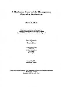
Fig. 2: A 4-stage MapReduce workflow.

example of such a workflow is shown in Fig. 2 which is composed of 4 stages, respectively with 8, 2, 4 and 1 (map or reduce) tasks. These tasks are to be scheduled on different nodes for parallel execution. However, in heterogeneous clouds, different nodes may have different performance and/or configuration specifications, and thus may have different service rates. Since resources are provisioned on-demand in cloud computing, the CSPs are faced with a general practical problem: how are resources to be selected and utilized for running each task in a cost-effective way? This problem is, in particular, directly relevant to CSPs wanting to compute their MapReduce workloads, especially when the computation budget is fixed. In this paper, we investigate the problem of scheduling a bag of MapReduce jobs within budget constraints. This bag of MapReduce jobs could be an iterative MapReduce job, a set of independent MapReduce jobs, or a collection of jobs related to some high-level applications such as Hadoop Hive [13]. We address task-level scheduling, which is fine grained compared to the frequentlydiscussed job-level scheduling, where the scheduled unit is a job instead of a task. Specifically, given a fixed amount of budget, we focus on how to efficiently select a machine from a candidate set for each task so that the total scheduling length of the job (aka makespan of the job) is minimum without breaking the budget. This problem is of particular interest to CSPs wanting to deploy MRaaS on heterogeneous cloud instances in a cost-effective way. To address this problem, we first design an efficient greedy algorithm for computing the minimum execution time with a given budget for each stage and show its optimality with respect to execution time and budget use. Then, with this result we develop a dynamic programming algorithm to achieve a global optimal solution within time of O(κB 2 ). To overcome the time complexity, we extend the idea in the greedy algorithm to efficient global distribution of the

IV

budget among the tasks in different stages for overall scheduling length reduction. Our empirical studies verify the proposed optimal algorithm and show the efficiency of the greedy algorithm to minimize the scheduling length. The rest of this paper is organized as follows: in Section 2, we introduce some background knowledge regarding the MapReduce framework and survey some related work. Section 3 formulates our problem. The proposed budgetdriven algorithms including the optimal and the greedy algorithms are discussed in Section 4. We follow with the results of our empirical studies in Section 5, and conclude the paper in Section 6.

2 Background and Related Work The MapReduce framework was first advocated by Google in 2004 as a programming model for its internal massive data processing [14]. Since then it has been widely discussed and accepted as the most popular paradigm for data intensive processing in different contexts. Therefore there are many implementations of this framework in both industry and academia (such as Hadoop [15], Dryad [16], Greenplum [17]), each with its own strengths and weaknesses. MapReduce is made up of an execution runtime and a distributed file system. The execution runtime is responsible for job scheduling and execution. It is composed of one master node and slave nodes. A distributed file system is used to manage task and data across nodes. When the master receives a submitted job, it first splits the job into a number of map and reduce tasks and then allocates them to the slave nodes, As with most distributed systems, the performance of the task scheduler greatly affects the scheduling length of the job, as well as, in our particular case, the budget consumed. There exists research on the scheduler of MapReduce aiming at improving its scheduling policies. For instance, Hadoop adopts speculative task scheduling to minimize the slowdown in the synchronization phases caused by straggling tasks in a homogeneous environment [15]. To extend this idea to heterogeneous clusters, Zaharia et al. [12] proposed the LATE algorithm. But this algorithm does not consider the phenomenon of dynamic loading, which is common in practice. This limitation was studied by You et al. [9] who proposed a loadaware scheduler. In addition, there are Other work on power-aware scheduling [18], deadline constraint scheduling [19], and scheduling based on automatic task slot assignments [20]. While these contributions do address different aspects of MapReduce scheduling, they are mostly centred on system performance and do not consider the budget, which is our main focus. Budget constraints have been considered in studies focusing on scientific workflow scheduling on HPC platforms including the Grid and Cloud [21–23].

V m



t1jl t2jl ... tjl jl



p1jl

p2jl

...

m pjl jl

 

Table 1: Time-price table of task Jjl

For example, Yu et al. [21] discussed this problem based on service Grids and presented a QoS-based workflow scheduling method to minimize execution cost and yet meet the time constraints imposed by the user. In the same vein, Zeng et al. [22] considered the executions of large scale many-task workflows in Clouds with budget constraints. They proposed ScaleStar, a budget-conscious scheduling algorithm to effectively balance execution time with the monetary costs. Now recall that, in the context of this paper, we view the executions of the jobs as a fork&join workflow characterized by multiple synchronized stages, each consisting of a collection of sequential or parallel map/reduce tasks. From this perspective, this abstract fork&join workflow can be viewed as a special case of general workflows. However, our focus is on MapReduce scheduling with budget constraints, rather than on general workflow scheduling. Therefore, the characteristics of MapReduce framework are fully exploited in the designs of the scheduling algorithms.

3 Problem Formulation 3.1

Workflow Model

We model a bag of MapReduce job as a multi-stage fork&join workflow that consists of κ stages (called a κ-stage job), each stage j having a collection of independent map or reduce tasks, denoted as Jj = {Jj0 , Jj1 , ..., Jjnj }, where 0 ≤ j < κ, and nj + 1 is the size of stage j. In a cloud, each map or reduce task may be associated with a set of machines that are provided by a cloud infrastructure provider to run this task, each machine with possibly distinct performance and configuration and thus with different charge rates. More specifically, for Task Jjl , 0 ≤ j < κ and 0 ≤ l ≤ nj the available machines and corresponding prices (service rates) are listed in Table 1, the values could be determined by the VM power and the computational loads of each task, where tujl , 1 ≤ u ≤ mjl represents the time to run task Jjl on machine Mu whereas pujl represents the corresponding price for using that machine, and mjl is the total number of the machines that can run Jjl . Without loss of generality, we assume that times have been sorted in increasing order and prices in decreasing order, and furthermore, that both time

VI

Table 2: Notation frequently used in model and algorithm descriptions Symbol Meaning

Symbol

κ Jji

the number of stages the ith task in stage j

mjl m

Jj nj n

task set in stage j the number of tasks in stage j the total number of tasks in the workflow time to run task Jjl on machine Mu Tj (Bj ) the shortest time to finish stage j given Bj the cost rate for using Mu T (B) the shortest time to finish the job given B

tujl pujl

Meaning

the total number of the machines the total size of time-price tables of the workflow Bjl the budget used by Jjl B the total budget for the MapReduce job Tjl (Bjl ) the shortest time to finish Jjl given Bjl

and price values are unique in their respective sorted sequence. These assumptions are reasonable since given any two machines with same run time for a task, the expensive one should never be selected. Similarly, given any two machines with same price for a task, the slow machine should never be chosen. For clarity and quick reference, we provide in Table 2 a summary of some symbols frequently used hereafter. 3.2

Budget Constraints

Given budget Bjl for task Jjl , the shortest time to finish it, denoted as Tjl (Bjl ) is defined as Tjl (Bjl ) = tujl

pu+1 < Bjl < pu−1 jl jl

(1)

m

Obviously, if Bjl < pjl jl , Tjl (Bjl ) = +∞. The time to complete a stage j with budget Bj , denoted as Tj (Bj ), is defined as the time consumed when the last task in that stage completes within the given budget: Tj (Bj ) = P

max

l∈[0,nj ] Bjl ≤Bj

{Tjl (Bjl )}

(2)

In fork&join, a stage cannot start until its immediately preceding stage has terminated. Thus the total makespan under budget B to complete the workflow is defined as the sum of all stages’ time. Our goal is to minimize the time within the given budget B. T (B) = P

min

j∈[0,κ) Bj ≤B

X

Tj (Bj )

(3)

j∈[0,κ)

Some readers may question the feasibility of this model since the number of stages and the number of tasks in each stage need to be known a prior to

VII

the scheduler. But, in reality, it is entirely possible since a) the number of map tasks for a given job is driven by the number of input splits (which is known to the scheduler) and b) the number of reduce tasks can be preset as with all other parameters (e.g., parameter mapred.reduce.tasks in Hadoop). As for the number of stages, it is not always possible to predefine it for MapReduce workflows. This is the main limitation of our model. But under the default FIFO job scheduler, we can treat a set of independent jobs as a single fork&join workflow. Therefore, we believe our model is still representative of most cases in reality.

4 Budget-Driven Algorithms In this section, we propose our task-level scheduling algorithms for MapReduce workflows with the goals of optimizing Equations (3) under budget constraints. To this end, we first leverage dynamic programming techniques to obtain an optimal solution and then present an efficient greedy algorithm to overcome its inherent complexity. 4.1

Optimization under Budget Constraints

The proposed algorithm should be able to distribute the budget among the stages, and in each stage distributing the assigned budget to each constituent task in an optimal way. To take these effects, we design the algorithm in two steps: 1. Given budget Bj for stage j, distribute the budget to all constituent tasks in such a way that Tj (Bj ) is minimum (see Equation (2)). Clearly, the computation for each stage is independent of other stages. Therefore such computations can be treated in parallel using κ machines. 2. Given budget B for a workflow and the results in Equation (2), optimize our goal of Equation (3). In-Stage Distribution To address the first step, we develop an optimal local greedy algorithm to distribute budget Bj between the nj + 1 tasks for stage j, 0 ≤ j ≤ κ − 1 in such a way that Tj (Bj ) is minimized. The idea of the algorithm is simple. To ensure that all the tasks in stage j have sufficient P budgetmto finish while minimizing Tj (Bj ), we first require Bj′ = Bj − l∈[0,nj ] pjl jl ≥ 0 and then iteratively distribute Bj′ in a greedy manner each time to the task whose current execution time determines Tj (Bj ) (i.e., the slowest one). This process continues until no sufficient budget is left. Clearly, having considered the structure of this problem, we can easily show its optimality with respect to minimizing the scheduling length within the given budget.

VIII

Global Distribution Given the results of the first step, we now consider the second step by using a dynamic programming recursion to compute the global optimal result. To this end, we use T (j, r) to represent the minimum total time to complete stages indexed from j to κ when budget r is available and use Tj [nj , q] to store the optimal time computed for stage j given budget q. Then, we have the following recursion (0 < j ≤ κ, 0 < r ≤ B): T (j, r) =

(

min {Tj (nj , q) + T (j + 1, r − q)} if j < κ

0 0

(6)

βj represents time saving on per-budget unit when task Jjl is moved from machine u to run on the next faster machine u − 1 in stage j (βj > 0) while βj′ is used when there are multiple slowest tasks in stage j (βj = 0). α is defined to allow βj to have a higher priority than βj′ in task selection. Put simply, unless for ∀j ∈ [1, κ], βj = 0 in which case βj′ is used, we use the value of βj , j ∈ [1, κ] as the criteria to select the allocated tasks. In the algorithm, all the values of the tasks in L are collected into a set V (Lines 19-28). We note that the tasks running on machine u = 1 in each stage have no definition of this value since they are already running on the fastest machine under the given budget (and thus no further improvement is available). Given set V , we can iterate over it to select the task in V that has the largest utility value, indexed by jl∗ , to be allocated budget for minimizing the stage computation time (Lines 29-30). We fist obtain the machine u to which the selected task is currently mapped and then compute the extra monetary cost δjl∗ if the task is moved from u to the next faster machine u − 1 (Lines 31-32). If the leftover budget B ′ is insufficient, the selected task will not be considered and removed from V (Line 40). In the next step, a task in a different stage will be selected for budget allocation (given each stage has at most one task in V ). This process will be continued until either the leftover budget B ′ is sufficient for a selected task or V becomes empty. In the former case, δjl∗ will be deducted from B ′ and added to the select task. At the same time, other profile information related to this allocation is also updated (Lines 33-37). After this, the algorithm exits from the loop and repeats the computation of L (Line 13) since L has been 3

Recall that the sequences of tujl and pujl are sorted, respectively in Table 1.

X

Opt(4) GGB(4) Opt(8) GGB(8)

700 600 500 400 300 200 1000

2000

3000

4000

Scheduling Time(s)

Scheduling Length

800

5000

Opt(16) GGB(16) Opt(32) GGB(32)

2500 2000 1500 1000 500 0

0.4 0.3 0.2 0.1 0 1000

2000

3000

4000

5000

5000

10000 Budget

15000

20000

15

0

5000

10000 Budget

15000

Scheduling Time(s)

Scheduling Length

3000

0.5

20000

10

5

0

0

Fig. 3: Impact of time-price table (TP) size on the scheduling length (e.g., makespan of the job in terms of indivisible time units) and the scheduling time (Stage:8, Task: ≤ 20/each stage, and the numbers in the brackets represent the different TP table sizes) changed due to this allocation. In the latter case, when V becomes empty, the algorithm returns directly, indicating that the final results of the budget distribution and the associated execution time of each tasks in each stage are available as recorded in the corresponding profile variables. Theorem 2. The time complexity of GGB is not greater than O(B(n+κ log κ)). In particular, when n ≥ κ log κ, the complexity of GGB is upper bounded by O(nB). Proof. The time complexity of this algorithm is largely determined by the nested loops (Lines 13-42). Since each allocation of budget B ′ is at least min {δjl }, 1≤≤κ,0≤l≤nj

B ), 1 ≤ j ≤ κ, 0 ≤ l ≤ nj iterations at Line the algorithm has at most O( min{δ jl } 13. On the other hand, if some advanced data structure such as a priority queue is used to optimize Pκ the search process, the algorithm can achieve a time complexity of O( j=1 log nj ) at Line 15 and O(κ log κ) at Line 29. Therefore, the overall time complexity can be written as

O(n +

κ X B ( log nj + κ log κ)) < O(B(n + κ log κ)) min{δjl } j=1

(7)

P − pujl , 1 ≤ j ≤ κ, 0 ≤ l ≤ nj and n = κj=1 nj the total where δjl = pu−1 jl number of tasks in the workflow. Here, we leverage the fact that log n < n.

XI

Obviously, when n ≥ κ log κ, which is reasonable in multi-stage MapReduce jobs, we obtain a time complexity of O(nB).

5 Empirical Studies To verify and evaluate the proposed algorithms and study their performance behaviours in reality, we developed a Budget Distribution Solver (BDS) in Java that efficiently implements the algorithms for the specified scheduling problem in MapReduce. Since the monetary cost is our primary interest, in BSD we did not consider some properties and features of the network platforms. Rather, we focus on the factors closely related to our research goal. In practical, how efficient the algorithms are in minimizing the scheduling lengths of the workflow subject to different budget constraints are our concern. The BDS accepts as an input a bag of MapReduce jobs that are organized as a multi-stage fork&join workflow by the scheduler at run-time. Each task of the job is associated with a time-price table, which is pre-defined by the cloud providers. As a consequence, the BDS can be configured with several parameters, including those described time-price tables, the number of tasks in each stage and the total number of stages in the workflow. Since there is no wellaccepted model to specify these parameters, we assume them to be automatically generated in a uniform distribution where the task execution time and the corresponding prices in particular are varied in the ranges of [1, 12.5*table size] and [1, 10*table size], respectively. As intuitively, with the table size being increased, the scheduler has more choices to select the candidate machines to execute a task. On the other hand, in each experiment we allow the budget resources to be increased from its lower bound to upper bound and thereby comparing the scheduling lengths and the scheduling time of the proposed algorithms with respect to different configuration parameters. Here, the lower and upper bound are defined to be the minimal and maximal budget resources, respectively, that can be used to complete the workflow. All the experiments are conducted by comparing the proposed GGB algorithm with the optimal algorithm Opt and the numerical results are obtained from a Ubuntu 12.04 platform having a hardware configuration of 3392.183 MHz processors, with a total of 8 processors activated, each with 8192K cache. 5.1

Impact of Time-Price Table Size

We first evaluate the impact of the time-price table size on the total scheduling length of the workflow with respect to different budget constraints. To this end, we fix a 8-stage workflow with at most 20 tasks in each stage. The size of the time-price table associated with each task varies from 4, 8, 16 to 32.

XII

The results of the GGB algorithm compared with those of the optimal algorithm are shown in Fig. 3. While the budget increases, for all sizes of the tables, the scheduling lengths decrease super-linearly. These results are interesting also difficulty to make from algorithm analysis alone. We attribute these results to the fact that the opportunities of reducing the execution time of each stage are super-linearly increased with the budget growth, especially for those large size workflows. This phenomenon implies that the performance/cost ratio increases if cloud users are willing to pay more for MapReduce computation. This figure also shows that the performance of GGB is very close to the optimal algorithm, but its scheduling time is significantly less than that of the optimal algorithm (quadratic in its time complexity). These results demonstrate how effective and efficient the proposed GGB algorithm is to achieve the best performance for MapReduce workflows subject to different budget constraints. 5.2

Impact of Workflow Size

In this set of experiments, we evaluate the performance changes with respect to different workflow sizes when the budget resources for each workflow are increased from the lower bound to the upper bound as we defined before. To this end, we fix the maximum number of tasks in the MapReduce workflow to 20 in each stage, and each task is associated with a time-price table with a maximum size of 16. We vary the number of stages from 4, 8, 16 to 32, and observe the performance and scheduling time changes in Fig. 4. From this figure, we can see that all the algorithms exhibit the same performance patterns with those we observed when the impact of the table size is considered. These results are expected as both the number of stages and the size of tables are linearly correlated with the total workloads in the computation. This observation can be also made when the number of tasks in each stage is changed.

6 Conclusions In this paper, we studied the scheduling of a bag of MapReduce jobs with budget constraints on a set of (virtual) machines in Clouds. To this end, we first presented a parallel optimal algorithm to address the constraints within pseudo polynomial time. The algorithm is based on dynamic programming techniques and integrates an in-stage local greedy algorithm to achieve the global optimality. To further improve the efficiency, we then developed a global greedy algorithm GGB that extends the idea of the local greedy algorithm to the distribution of the budget among the tasks across different stages of the workflow while

XIII 3 Scheduling Time(s)

Scheduling Length

2000 1500 1000 500 0

0

2000

4000

6000

5000

Scheduling Time(s)

Scheduling Length

1 0.5 0

2000

4000

6000

8000

150

6000

4000 3000 2000 1000 0

2 1.5

0

8000

Opt(4) GGB(4) Opt(8) GGB(8)

2.5

0

5000 10000 15000 20000 25000 30000 Budget

Opt(16) GGB(16) Opt(32) GGB(32)

100

50

0

0

5000 10000 15000 20000 25000 30000 Budget

Fig. 4: Impact of the number of stages on the total scheduling length (e.g., makespan of the job in terms of indivisible time units) and scheduling time (Task: ≤ 20, Table Size ≤ 16, and the numbers in the brackets represent the different number of stages) minimizing the scheduling length as a goal. The performance of the proposed algorithms were evaluated by empirical studies. The results show that the GGB is close to the optimal results in terms of the scheduling length but entails much lower time overhead.

References 1. Hoffa, C., Mehta, G., Freeman, T., Deelman, E., Keahey, K., Berriman, B., Good, J.: On the use of cloud computing for scientific workflows. In: eScience, 2008. eScience ’08. IEEE Fourth International Conference on. (dec 2008) 640 –645 2. Juve, G., Deelman, E., Berriman, G.B., Berman, B.P., Maechling, P.: An evaluation of the cost and performance of scientific workflows on amazon ec2. J. Grid Comput. 10(1) (mar 2012) 5–21 3. Dean, J., Ghemawat, S.: Mapreduce: simplified data processing on large clusters. Commun. ACM 51(1) (January 2008) 107–113 4. Liu, H., Orban, D.: Cloud mapreduce: A mapreduce implementation on top of a cloud operating system. In: Cluster, Cloud and Grid Computing (CCGrid), 2011 11th IEEE/ACM International Symposium on. (2011) 464–474 5. Ibrahim, S., Jin, H., Lu, L., Qi, L., Wu, S., Shi, X.: Evaluating mapreduce on virtual machines: The hadoop case. In: Proceedings of the 1st International Conference on Cloud Computing. CloudCom ’09 (2009) 519–528 6. Correia, M., Costa, P., Pasin, M., Bessani, A., Ramos, F., Verissimo, P.: On the feasibility of byzantine fault-tolerant mapreduce in clouds-of-clouds. In: Reliable Distributed Systems (SRDS), 2012 IEEE 31st Symposium on. (2012) 448–453

XIV 7. Marozzo, F., Talia, D., Trunfio, P.: Enabling reliable mapreduce applications in dynamic cloud infrastructures. ERCIM News 2010(83) (2010) 44–45 8. Zaharia, M., Borthakur, D., Sen Sarma, J., Elmeleegy, K., Shenker, S., Stoica, I.: Delay scheduling: a simple technique for achieving locality and fairness in cluster scheduling. In: Proceedings of the 5th European conference on Computer systems. EuroSys ’10 (2010) 265– 278 9. You, H.H., Yang, C.C., Huang, J.L.: A load-aware scheduler for mapreduce framework in heterogeneous cloud environments. In: Proceedings of the 2011 ACM Symposium on Applied Computing. SAC ’11 (2011) 127–132 10. Li, Y., Zhang, H., Kim, K.H.: A power-aware scheduling of mapreduce applications in the cloud. In: Dependable, Autonomic and Secure Computing (DASC), 2011 IEEE Ninth International Conference on. (2011) 613–620 11. Kondikoppa, P., Chiu, C.H., Cui, C., Xue, L., Park, S.J.: Network-aware scheduling of mapreduce framework ondistributed clusters over high speed networks. In: Proceedings of the 2012 workshop on Cloud services, federation, and the 8th open cirrus summit. FederatedClouds ’12 (2012) 39–44 12. Zaharia, M., Konwinski, A., Joseph, A.D., Katz, R., Stoica, I.: Improving mapreduce performance in heterogeneous environments. In: Proceedings of the 8th USENIX conference on Operating systems design and implementation. OSDI’08 (2008) 29–42 13. Thusoo, A., Sarma, J., Jain, N., Shao, Z., Chakka, P., Zhang, N., Antony, S., Liu, H., Murthy, R.: Hive - a petabyte scale data warehouse using hadoop. In: Data Engineering (ICDE), 2010 IEEE 26th International Conference on. (2010) 996–1005 14. Dean, J., Ghemawat, S.: Mapreduce: simplified data processing on large clusters. In: Proceedings of the 6th conference on Symposium on Opearting Systems Design & Implementation - Volume 6. OSDI’04 (2004) 10–10 15. : Apache Software Foundation. Hadoop, http:/hadoop.apache.org/core. 16. Isard, M., Budiu, M., Yu, Y., Birrell, A., Fetterly, D.: Dryad: distributed data-parallel programs from sequential building blocks. In: Proceedings of the 2nd ACM SIGOPS/EuroSys European Conference on Computer Systems 2007. EuroSys ’07 (2007) 59–72 17. : Greenplum HD, http:/www.greenplum.com. 18. Li, Y., Zhang, H., Kim, K.H.: A power-aware scheduling of mapreduce applications in the cloud. In: Dependable, Autonomic and Secure Computing (DASC), 2011 IEEE Ninth International Conference on. (2011) 613–620 19. Kc, K., Anyanwu, K.: Scheduling hadoop jobs to meet deadlines. In: Cloud Computing Technology and Science (CloudCom), 2010 IEEE Second International Conference on. (2010) 388–392 20. Wang, K., Tan, B., Shi, J., Yang, B.: Automatic task slots assignment in hadoop mapreduce. In: Proceedings of the 1st Workshop on Architectures and Systems for Big Data. ASBD ’11 (2011) 24–29 21. Yu, J., Buyya, R.: Scheduling scientific workflow applications with deadline and budget constraints using genetic algorithms. Sci. Program. 14(3,4) (December 2006) 217–230 22. Zeng, L., Veeravalli, B., Li, X.: Scalestar: Budget conscious scheduling precedenceconstrained many-task workflow applications in cloud. In: Proceedings of the 2012 IEEE 26th International Conference on Advanced Information Networking and Applications. AINA ’12 (2012) 534–541 23. Caron, E., Desprez, F., Muresan, A., Suter, F.: Budget constrained resource allocation for non-deterministic workflows on an iaas cloud. In: Proceedings of the 12th international conference on Algorithms and Architectures for Parallel Processing - Volume Part I. ICA3PP’12 (2012) 186–201

XV

Algorithm 1 Global-Greedy-Budget Algorithm (GGB) 1: procedure T (1,P B) 2: B ′ = B − j∈[1,κ] Bj′ 3: if B ′ < 0 then return (+∞) 4: end if 5: 6: for j ∈ [1, κ] do 7: for Jjl ∈ Jj do m 8: Tjl ← tjl jl m 9: Bjl ← pjl jl 10: Mjl ← mjl 11: end for 12: end for 13: while B ′ ≥ 0 do 14: 15: 16:

L←∅ for j ∈ [1, κ] do < jl, jl′ >∗ ← arg max{Tjl (Bjl )}

17: 18: 19: 20: 21: 22: 23: 24: 25: 26: 27: 28: 29: 30:

L ← L ∪ {< jl, jl′ >∗ } end for V ←∅ for < jl, jl′ >∈ L do u ← Mjl if u > 1 then u < pu−1 jl , pjl >← Lookup(Jjl , u − 1, u) u vjl ← αβj + (1 − α)βj′ u V ← V ∪ {vjl } end if end for while V 6= ∅ do

⊲ Dist. B among κ stages P m ⊲ Bj′ = l∈[0,nj ] pjl jl

⊲ No sufficient budget! ⊲ Initialization P ⊲ O( κj=1 nj ) = # of tasks

⊲ record exec. time ⊲ record budget dist. ⊲ record assigned machine index.

B

⊲ ≤ O( min

1≤j≤κ,0≤l≤nj {δjl }

⊲ O(

l∈[0,nj ]

Pκ

j=1

)

log nj )

⊲ |L| = κ

⊲ O(κ)

⊲ |V | ≤ κ

⊲ O(κ log κ) ⊲ sel. task with max. u.value

u jl∗ ← arg max{vjl } u ∈V vjl

31: u ← Mjl∗ u 32: δjl∗ ← pu−1 jl∗ − pjl∗ ′ 33: if B ≥ δjl∗ then 34: B ′ ← B ′ − δjl∗ 35: Bjl∗ ← Bjl∗ + δjl∗ 36: Tjl∗ ← tu−1 jl∗ 37: Mjl∗ ← u − 1 38: break 39: else u 40: V ← V \ {vjl ∗} 41: end if 42: end while 43: if V = ∅ then 44: return 45: end if 46: end while 47: end procedure

⊲ Lookup matrix in Table 1 ⊲u>1 ⊲ reduce Jjl∗ ’s time

⊲ restart from scratch ⊲ select the next one in V

⊲ Bj =

P

l∈[0,nj ]

Bjl