Amazon added a new service, called Amazon Elastic MapReduce to enable businesses, re- searchers, data ..... command line tools. Table I ..... [22] S. Seo, I. Jang, K. Woo, I. Kim, J. Kim, S. Maeng, âHPMR: Prefetching and Pre-. Shuffling in ...
Locality-Aware Reduce Task Scheduling for MapReduce Mohammad Hammoud and Majd F. Sakr Carnegie Mellon University in Qatar Education City, Doha, State of Qatar Email: {mhhammou,msakr}@qatar.cmu.edu
Abstract—MapReduce offers a promising programming model for big data processing. Inspired by functional languages, MapReduce allows programmers to write functional-style code which gets automatically divided into multiple map and/or reduce tasks and scheduled over distributed data across multiple machines. Hadoop, an open source implementation of MapReduce, schedules map tasks in the vicinity of their inputs in order to diminish network traffic and improve performance. However, Hadoop schedules reduce tasks at requesting nodes without considering data locality leading to performance degradation. This paper describes Locality-Aware Reduce Task Scheduler (LARTS), a practical strategy for improving MapReduce performance. LARTS attempts to collocate reduce tasks with the maximum required data computed after recognizing input data network locations and sizes. LARTS adopts a cooperative paradigm seeking a good data locality while circumventing scheduling delay, scheduling skew, poor system utilization, and low degree of parallelism. We implemented LARTS in Hadoop-0.20.2. Evaluation results show that LARTS outperforms the native Hadoop reduce task scheduler by an average of 7%, and up to 11.6%.
I. I NTRODUCTION Intel predicts the Era of Tera is coming quickly [3]. How to effectively process sheer volumes of data and facilitate dataintensive tasks for applications such as web indexing, machine learning, and astronomical data parsing is becoming a major challenge. In many such situations, the required processing power exceeds the capabilities of individual computers imposing the use of distributed computing. MapReduce [4] created by Google presents a potential solution. MapReduce is a programming model for large-scale dataintensive distributed data processing. It provides minimal abstractions, hides architectural details, automatically parallelizes computation, and supports transparent fault tolerance via replication. Google utilizes MapReduce to process 20 petabytes of data per day [4]. Amazon added a new service, called Amazon Elastic MapReduce to enable businesses, researchers, data analysts, and developers to easily and costeffectively process vast amounts of data [1]. Since its debut on the computing stage, MapReduce has frequently been associated with Hadoop [6]. Hadoop [9] is an open source implementation of MapReduce and is currently enjoying wide popularity. As an engine to power the cloud, industry’s premier web vendors- Facebook, Google, Microsoft, and Yahoo!- have advocated Hadoop [15]. Likewise, academia has started using Hadoop for seismic simulation, natural language processing, and web data mining, among others [26].
Hadoop presents MapReduce as an analytics engine and under the hood uses a distributed storage layer referred to as Hadoop Distributed File System (HDFS). HDFS mimics Google File System (GFS) [13]. A main characteristic of MapReduce is simplicity which allows programmers to write functional-style code. A user submits a job comprising of a map function and a reduce function which are subsequently transformed into map and reduce tasks scheduled on slots hosted by participating nodes in the cluster. HDFS loads, partitions data into fixed equal-size splits, and distributes splits across cluster nodes. Each split is assigned a map task. Map tasks process splits and produce intermediate outputs that are usually partitioned/hashed to one or many reduce tasks. Each reduce task collects/shuffles its corresponding partitions (i.e., the intermediate outputs from feeding nodes1 ) from one or many nodes, merges them, applies the user-provided reduce function, and produces final results. MapReduce assumes a master-slave architecture and a treestyle network topology. Nodes are spread over different racks encompassed in one or many data centers. A salient point is that the bandwidth between two nodes is dependent on their relative locations in the network topology. For example, nodes that are on the same rack have higher bandwidth between them as opposed to nodes that are off-rack. As such, it pays to minimize data shuffling across racks. The master in MapReduce is responsible for scheduling map and reduce tasks at slave nodes after receiving requests from slaves for that regard. Hadoop attempts to schedule map tasks in proximity to input splits in order to avoid transferring them over the network. In contrast, Hadoop schedules reduce tasks at requesting slaves without any data locality consideration. As a result, unnecessary data might get shuffled on the network causing performance degradation. Moving data repeatedly to distant nodes is becoming the bottleneck [23]. In this paper we rethink reduce task scheduling in Hadoop and suggest making Hadoop’s reduce task scheduler aware of partitions’ network locations and sizes in order to mitigate network traffic. We propose LocalityAware Reduce Task Scheduler (LARTS), a practical strategy that leverages network locations and sizes of partitions to exploit data locality. In particular, LARTS attempts to schedule reducers as close as possible to their maximum amount of 1 A feeding node of a reducer, R, is a node that hosts at least one of R’s feeding map tasks.
input data and conservatively switches to a relaxation strategy seeking a balance between scheduling delay, scheduling skew, system utilization, and parallelism. Evaluations demonstrate LARTS’s outperformance over native Hadoop. In this work we make the following contributions: • We propose a novel strategy, LARTS, which applies data locality to reduce task scheduling in MapReduce. • We empirically analyze Hadoop’s performance and network traffic. We observe that the process of interleaving the execution of map tasks with the shuffling of partitions employed by native Hadoop improves performance but increases network traffic. We show how LARTS manages to maintain the advantage of the interleaving process besides diminishing network traffic. • We implemented LARTS in Hadoop 0.20.2 and conducted extensive experimentations to evaluate its potential. We found that LARTS improves node-local, racklocal, and off-rack traffic by 34.45%, 0.32%, and 7.5%, on average, versus native Hadoop. In summary, LARTS outperforms native Hadoop by an average of 7%, and up to 11.6%. The rest of the paper is organized as follows. A background on Hadoop’s scheduling is given in Section II. We analyze Hadoop’s incurred network traffic and performance in Section III. Section IV describes LARTS. We evaluate LARTS in Section V. Finally, we provide a summary of prior related work in Section VI and conclude in Section VII. II. BACKGROUND : S CHEDULING IN H ADOOP The master node in MapReduce is referred to as Job Tracker (JT). Each slave node is denoted as Task Tracker (TT). JT and TTs communicate over the cluster network via a heartbeat mechanism. Hadoop’s framework adopts a pull scheduling strategy rather than a push one. That is, JT does not push map and reduce tasks to TTs but rather TTs pull them by making pertaining requests. Every TT sends a heartbeat message periodically to JT encompassing a request for a map or a reduce task to run. JT satisfies requests for map tasks via attempting to schedule mappers in the vicinity of their input splits. However, JT simply assigns the next yet-to-run reduce task to a requesting TT regardless of TT’s network location and its implied effect on the reducer’s shuffle time. III. E ARLY S HUFFLE IN H ADOOP As a mechanism to improve performance, Hadoop schedules a reducer before every corresponding partition is available. In particular, the reduce task scheduler is activated after only a certain percentage (default 5%) of mappers commit. The rationale behind such a process is to interleave the execution of mappers with the shuffling of partitions and enhance, consequently, the turnaround time of MapReduce jobs. We refer to this technique as early shuffle. The early shuffle process affects the decisions made by LARTS, hence, analyzed in this section. We evaluated several benchmarks on native Hadoop by turning early shuffle on (H ESON) and off (H ESOFF)2 . We 2 The utilized experimentation environment and benchmarks are described in Section V.
Rack0
PR0:TT0 = 40MB
TT0
PR1:TT1 = 30MB
TT1
ask eT
c
u ed
Rack2 st
ue
eq
1.R
aR
wit ply
1
hR
Re
JT Rack1 Re
ply
2.R
eq ue
st
wi
th
aR
ed
R0
PR1:TT2 = 50MB
TT2
PR1:TT3 = 30MB PR0:TT3 = 35MB
TT3
uc
eT as
k
Fig. 1. An example of two Task Trackers making requests for reduce tasks in native Hadoop (JT = Job Tracker, TTj = Task Tracker j, Ri = reducer i, and PRi:T T j = partition P produced at TTj and hashed to reducer, Ri).
modified Hadoop 0.20.2 to filter out reduce traffic into nodelocal, rack-local, and off-rack. Specifically, node-local traffic is incurred after a reducer, R, is scheduled at a node hosting a partition to be consumed by R. Rack-local traffic is incurred after a partition is shuffled to R from a feeding node that is on the same rack as R’s node. Off-rack traffic is incurred after a partition is shuffled to R from an off-rack feeding node. We observed that H ESOF maximizes node-local traffic by an average of 26.8% compared to H ESON. Furthermore, H ESOF minimizes rack-local and off-rack traffic by 2.5% and 1.2%, on average, respectively versus H ESON. Nonetheless, we realized that H ESON outperforms H ESOFF by an average of 9.2%. Hadoop adopts a resource estimator that estimates the input size of each reducer, R, before R is scheduled. If Hadoop finds that a requesting Task Tracker, TT, does not have enough space to run R, R is not scheduled at TT (i.e., TT is rejected). With early shuffle on, reducers are scheduled while mappers are running. When mappers are running they consume system resources. Busy mappers will essentially consume resources more, and will produce larger amounts of intermediate outputs. As such, the likelihood that the Job Tracker rejects requests for reducers from TTs hosting busy mappers increases. Subsequently, when the busy mappers complete, their generated outputs will require shuffling to corresponding reducers which have been potentially scheduled at different nodes. Clearly, this incurs more traffic on the network. In contrast, with early shuffle being off, mappers and reducers run asynchronously. Therefore, the likelihood that the Job Tracker schedules reducers at the Task Trackers that were accommodating busy mappers increases, avoiding thereby shuffling large partitions. This explains why H ESOFF experiences less network traffic than H ESON as indicated earlier. On the other hand, via running mappers and reducers synchronously, H ESON minimizes jobs’ turnaround times. Because the gain from decreased jobs’ turnaround times offsets the loss from increased network traffic, H ESON outperforms H ESOFF. We describe in Section IV-B how LARTS intelligently combines the advantages of H ESON and H ESOFF and abandons their disadvantages, thus boosting MapReduce performance.
This section begins by first motivating the problem and then describing LARTS’s paradigm. A. Motivation Fig. 1 demonstrates a simple example of two Task Trackers requesting reduce tasks, R0 and R1, from the Job Tracker (JT) in native Hadoop. TTj stands for a Task Tracker node j. PRi:T T j stands for a partition P produced at TTj and hashed to reducer, Ri. JT might receive requests from TT0 and TT3 and reply with R1 and R0, respectively. This incurs shuffling PR0:T T 0 from TT0 to TT3, PR1:T T 2 from TT2 to TT0, and PR1:T T 3 from TT3 to TT0 (i.e., 120MB off-rack traffic, in aggregate). In addition, PR1:T T 1 will be shuffled from TT1 to TT0 (i.e., 30MB rack-local traffic) and PR0:T T 3 will remain local to TT3 (i.e., 35MB node-local traffic). On the other hand, if JT schedules R0 at TT0 and R1 at TT3, PR0:T T 3 will be shuffled from TT3 to TT0, PR1:T T 1 from TT1 to TT3 (i.e., 65MB off-rack traffic, in aggregate), PR1:T T 2 from TT2 to TT3 (i.e., 50MB rack-local traffic), and PR0:T T 0 and PR1:T T 3 will remain local to TT0 and TT3, respectively (i.e., 70MB node-local traffic, in aggregate). Clearly, scheduling R0 at TT0 and R1 at TT3 improves node-local, rack-local, and off-rack traffic by 50%, 40%, and 45.8% versus scheduling them at TT3 and TT0, respectively. More notably, if JT does not schedule R1 at TT3 but rather wait (a little time) to receive a request from TT2 and schedule R1 there, node-local and rack-local traffics will be further improved by 22.2% and 40%, respectively. Hadoop, in its present design, is incapable of making such scheduling decisions.
upon when to start early shuffle depends on the observed performance. We advocate starting early shuffle after a defined number, ES, of mappers are done. We define a sweet spot of a program as the spot at which early shuffle is triggered and provides the best performance for the program. We can alter ES for any application to locate its sweet spot. At a sweet spot, a reducer would have already recognized all its partitions or approximately all. Locating a sweet spot introduces a tradeoff between reaping early shuffle’s benefit and delivering fully accurate information (i.e., network locations of partitions) to LARTS. The attained accuracy depends essentially on workloads’ characteristics and their underlying data sets. Section V-C provides an extensive sensitivity study on locating sweet spots for multiple benchmarks. Through the usage of sweet spots, LARTS can sensibly combine the advantages of H ESON and H ESOFF and abandon their disadvantages (see Section III for details on H ESON and H ESOFF). 70
Min Max
60
Average 50
Partition Sizes (MB)
IV. T HE LARTS TASK S CHEDULER
40
30
20
10
0 1
2
3
4
5
6
7
8
9
10 11 12 13 14 15 16 17 18 19 20 21 22 23 24 25
Reducer ID
B. LARTS and Early Shuffle A key question is how to schedule reduce tasks at Task Trackers so as to diminish shuffled data and improve MapReduce performance. One of Hadoop’s basic principles is: ”moving computation towards data is cheaper than moving data towards computation”. Such a principle is employed by Hadoop when scheduling map tasks but bypassed when scheduling reduce tasks. MapReduce is aware of the network locations of splits (inputs to mappers) and leverages such information to schedule mappers nearby splits. In contrast, MapReduce is oblivious to the network locations of partitions (inputs to reducers) and does not schedule reducers nearby partitions. Thus, similar to map task scheduling, we suggest making MapReduce aware of partitions’ network locations in order to apply locality to reduce task scheduling. Any reducer can receive a partition from any mapper. As such, to certainly designate all the network locations of a reducer’s partitions, we need to wait until all mappers complete. When the map phase is fully done, all the network locations of the feeding nodes of every reducer will be known. Evidently, to meet such an objective, we need to disable early shuffle. Disabling early shuffle, however, prevents us from exploiting its advantage (i.e., decreased jobs’ turnaround times). Hence, we propose waiting for all mappers to complete only if required (more on this shortly), and activating early shuffle at an earlier stage if possible. The criterion in deciding
Fig. 2. Skew in partitions of sort2. Min, Max, and Average denote the minimum, the maximum, and the average sizes of partitions sent by each feeding mapper to each reducer.
Lastly, in addition to network locations, MapReduce has to recognize partitions’ sizes in order to apply locality to reduce task scheduling. Contrary to splits, partitions are of variable sizes. For instance, Fig. 2 shows the maximum, the minimum, and the average sizes of partitions delivered by each feeding mapper to each reducer in the sort2 program (see Section V-A for details on this benchmark). Clearly, this workload exhibits a significant discrepancy between the sizes of partitions consumed by reducers. Keeping large partitions and shuffling smaller ones (if possible) saves network bandwidth. As such, LARTS incorporates partitions’ sizes in reduce task scheduling in an endeavor to avoid transferring large partitions. C. Maximum-Racks and Maximum-Nodes: Locality and Tradeoffs As described in Section I, the amount of data shuffled depends on where reducers are scheduled. In case a reducer, R, has only one feeding mapper, M, the best data locality can be achieved via scheduling R at the Task Tracker that hosts M. However, R typically has multiple feeding mappers which are usually located at multiple nodes. We suggest that good data locality can be achieved via scheduling R at the maximum-node in the maximum-rack of R. We define the maximum-rack of R as the rack that holds one or many of R’s partitions with an
aggregate size larger than any other aggregate sizes of other R’s partitions held at other racks. In addition, we define the maximum-node of R as the node that holds the largest partition for R at R’s maximum-rack. We identify the maximum-node and the maximum-rack of R using the network locations and sizes of R’s partitions. Existing Hadoop adopts a pull scheduling strategy rather than a push one (see Section II for details). Consequently, scheduling every reducer, R, at its maximum-node in its maximum-rack might cause scheduling delay, scheduling skew, low degree of parallelism, and poor system utilization. Scheduling delay occurs when many Task Trackers request R and get rejected because none of them is found preferred by R (i.e., none is R’s maximum-node in R’s maximumrack). Principally, this means that the Job Tracker will not schedule R at any Task Tracker but the one that is preferred by R. Furthermore, the Job Tracker will keep watching for R’s preferred Task Tracker to make a request so that it schedules R there. Obviously, this might introduce some scheduling delay. Scheduling skew refers to the variance in Task Trackers being preferred by reducers. Low degree of parallelism and poor system utilization occur after a skew in scheduling. That is, available slots at Task Trackers not preferred by any reducer will remain unutilized and will entail less exploited parallelism. D. Relaxation and Maximum-Nodes
Best
Effort
Maximum-Racks
and
Algorithm 1 LARTS Algorithm RT : set of unscheduled reduce tasks T T : the task tracker requesting a reduce task RCT T : the rejection counter associated with T T Output: A reduce task R ∈ RT that can be scheduled at T T 1: initialize two sets of potential reducers to schedule at T T , setOnRack = Φ and setOf f Rack = Φ 2: for every reduce task R ∈ RT do 3: calculate maximum-rack M RR = max{rack holding partitions f or R} 4: calculate maximum-node M NR = max{f eeding node in M RR } 5: if T T ∈ M RR && T T = M NR then 6: return R 7: else 8: if T T ∈ M RR && RCT T = α then 9: add R to setOnRack 10: else 11: if RCT T > α then 12: add R to setOf f Rack 13: end if 14: end if 15: end if 16: end for 17: if setOnRack is not empty then 18: return a random reducer R ∈ setOnRack 19: else 20: if setOf f Rack is not empty then 21: return a random reducer R ∈ setOf f Rack 22: end if 23: end if Input:
LARTS balances scheduling delay, scheduling skew, system utilization, and parallelism by judiciously fragmenting some reduce tasks among several requesting Task Trackers. We
Rack0
PR0:TT0 = 40MB
TT0
PR1:TT1 = 30MB
TT1
ask eT
Rack2 JT RCTT0 = 0 RCTT1 = 1 RCTT2 = 0 RCTT3 = 1
uc ed aR 0 R est qu with e ask 1.R eply eT R uc ed R a st ue eq 2.R
4.Re
ques t
Reply
3.Re q
Rack1 a Re
with
uest a
duce
R1
Task
Redu
PR1:TT2 = 50MB
TT2
PR1:TT3 = 30MB PR0:TT3 = 35MB
TT3
ce Ta s
k
Fig. 3. An example of Task Trackers making requests for reduce tasks in LARTS. The Job Tracker rejects requests from Task Trackers 1 and 3 because they don’t satisfiy LARTS’s conditions (JT = Job Tracker, TTj = Task Tracker j, RCT T j = rejection counter associated with TTj, Ri = reducer i, and PRi:T T j = partition P produced at TTj and hashed to reducer, Ri).
introduce a rejection counter, RC, per each Task Tracker, TT (i.e., RCT T ) and increment it each time TT gets rejected by the Job Tracker. We further define a threshold, α, through which we bound RC. We gradually then start relaxing the condition of maximum-node in maximum-rack for R. Specifically, LARTS first attempts to strictly meet the condition of maximum-node in maximum-rack for R. However, after RCT T of a requesting TT reaches α, LARTS relaxes the condition on TT to only satisfying being on the maximum-rack of R. In addition, if RCT T becomes greater than α, LARTS relaxes every condition on TT and simply assigns it a random R. In summary, LARTS exerts best effort in meeting the maximum-node in maximum-rack condition for every reducer, but gradually starts applying a relaxation strategy in order to avoid scheduling delay, scheduling skew, potential poor utilization, and probable low degree of parallelism. To that end, Algorithm 1 formally describes LARTS. E. A Working Example Fig. 3 demonstrates a simple working example of two Task Trackers requesting reduce tasks, R0 and R1, from the Job Tracker (JT) in LARTS. We assume an α of 1. As in Fig. 1, TTj stands for a Task Tracker node j. PRi:T T j stands for a partition P produced at TTj and hashed to reducer, Ri. RCT T j refers to the rejection counter associated with Task Tracker TTj. As shown, JT receives first a request for a reduce task from TT0. JT realizes that R1 does not prefer TT0 but R0 does (i.e., TT0 is the maximum-node in the maximum-rack of R0). As such, JT assigns R0 to TT0. This incurs only shuffling PR0:T T 3 from TT3 to TT0 while PR0:T T 0 is kept local to TT0. JT receives a second request for a reduce task from TT1 and rejects the request because the remaining reducer, R1, does not prefer TT1. Consequently, JT increments RCT T 1 by 1. A third request for a reduce task is received by JT from TT3. Though TT3 belongs to the maximum-rack of R1, it is neither the maximum-node of R1 nor has yet a rejection counter evaluating to α. Consequently, JT rejects TT3 and increments RCT T 3 by 1. Lastly, JT receives a fourth request for a reduce task from TT2 and replies with R1 because TT2 is R1’s maximum-node in R1’s maximum-rack. As a
RAM/Blade Storage/Blade Virtualization Platform VM Parameters
OS JVM Hadoop
We evaluate LARTS against native Hadoop on our cloud computing infrastructure comprised of a dedicated 14 physical host IBM BladeCenter H with identical hardware, software and network capabilities. The BladeCenter is configured with the VMware vSphere 4.1 virtualization environment. VMware vSphere 4.1 [24] manages the overall system and VMware ESXi 4.1 runs as the blades’ hypervisor. The vSphere system was configured with a single virtual machine (VM) running on each BladeCenter blade. Each VM is configured with 4 v-CPUs and 4GBs of RAM. The disk storage for each VM is provided via two locally connected 300GB SAS disks. The major system software on each VM is 64-bit Fedora 13 [7], Apache Hadoop 0.20.2 [9] and Sun/Oracle’s JDK 1.6 [5], Update 20. To employ Hadoop’s rack awareness correctly, blades 1-7 are connected to a 1 gigabit switch, blades 8-14 to another 1 gigabit switch, and the two switches are connected to a third 1 gigabit switch providing interconnectivity for all blades. All the switches are physical. Lastly, LARTS research is monitored with the Ganglia cluster monitoring system [8], the VMware vSphere client application, and standard Linux command line tools. Table I summarizes our cloud hardware configuration and software parameters. To evaluate LARTS against native Hadoop, we use the sort and the wordcount benchmarks in the Hadoop distribution. Sort is the main benchmark used for assessing Hadoop at Yahoo! [26]. Sort was also used in the MapReduce Google’s paper [4]. Besides, [22] reported that wordcount is as well one of the major benchmarks utilized for evaluating Hadoop at Yahoo!. To test LARTS with various types of data sets, we ran sort over two data sets, one with uniform (the default) and another with non-uniform keys frequencies and data distribution across nodes. To generate a uniform data set we simply generate records with random keys and equal number of records at
TABLE II B ENCHMARK PROGRAMS Key Frequency Uniform Non-Uniform Real Log Files
Benchmark sort1 sort2 wordcount
Data Distribution Uniform Non-Uniform Real Log Files
Dataset Size 14 GB 13.8 GB 11 GB
Map Tasks 238 228 11
Reduce Tasks 25 25 3
To produce a skew in data distribution we allowed each mapper running at a different node to generate records between two limits, high and low. As the difference between the two limits increases, the skew in data distribution also increases. With a low limit of 0.5GB and a high one of 1.5GB we were able to produce a skew in data distribution with a variance of 34%. Consequently, we obtain a data set with non-uniform keys frequencies and data distribution across nodes. We refer to sort running on this non-uniform data set as sort2. Lastly, we applied wordcount to a set of real system log files. Though wordcount is a map-bound program, it is very useful to use in order to verify how LARTS affects map-bound applications while it targets reduce task scheduling. Table II illustrates our utilized benchmarks. To account for variances across runs we ran each benchmark 5 times. 2A98D4A;=E#
6=;@D4A;=E#
1FD6=;@#
$!!"# ,!"# +!"# *!"# )!"# (!"# '!"# &!"# %!"# $!"# !"#
0A?0'@BB"
+3456789":;5869J$ %!#$ %!&$ %'#$ %'&$ %&#$ %&&$ !"#$
()*&+$,-*&.&#/$ ()*'+$,-*&.&#/$ ()*!+$,-*&.&#/$
()*&+$,-*&.!/$ ()*'+$,-*&.!/$ ()*!+$,-*&.!/$
()*&+$,-*&.2/$ ()*'+$,-*&.2/$ ()*!+$,-*&.2/$
()*&+$,-*&.1/$ ()*'+$,-*&.1/$ ()*!+$,-*&.1/$
()*&+$,-*&.0/$ ()*'+$,-*&.0/$ ()*!+$,-*&.0/$
()*&+$,-*&."/$ ()*'+$,-*&."/$ ()*!+$,-*&."/$
Sweet Spot
()*&+$,-*'.&/$ ()*'+$,-*'.&/$ ()*!+$,-*'.&/$
sweet spots (shown in Section V-C) for all the benchmarks under LARTS. Since we ran each benchmark 5 times, we display the average results for each program. We start by showing in Fig. 4 node-local, rack-local, and off-rack traffic generated by H ESON, H ESOFF, and LARTS for all the benchmarks. As demonstrated and discussed in Section III, H ESOFF does better than H ESON concerning incurred network traffic. LARTS, on the other hand, is superior to both, H ESON and H ESOFF. Through applying the maximumnode in maximum-rack and the maximum-rack after a Task Tracker’s rejection counter reaches α conditions, LARTS maximizes node-local, maximizes/minimizes rack-local, and minimizes off-rack traffic. LARTS minimizes rack-local traffic only after maximizing node-local traffic. For instance, assume a reducer, R, with a single feeding mapper, M. Scheduling R on M’s node versus on M’s rack but not on M’s node maximizes node-local and minimizes rack-local traffic. For the tested benchmarks, LARTS maximizes node-local and rack-local traffic by 34.45% and 0.32%, and minimizes offrack traffic by 7.5%, on average, against H ESON. Besides, LARTS maximizes node-local and rack-local traffic by 16.7% and 2.8%, and minimizes off-rack traffic by 6.3%, on average, against H ESOFF. Fig. 5 shows the corresponding execution time results for the three benchmarks under H ESON, H ESOFF, and LARTS. As discussed in Section III, H ESON outperforms H ESOFF. On the other hand, LARTS surpasses both, H ESON and H ESOFF via sensibly combining the advantages of H ESON and H ESOFF and abandoning their disadvantages (see Section IV-B for details). LARTS still employs early shuffle- yet conservatively, and, moreover, reduces network traffic. LARTS outperforms H ESON and H ESOFF by 7% and 15.4%, on average, and up to 11.6% and 25.2%, respectively. Finally, though wordcount exposes more reduction in network traffic under LARTS than sort1 and sort2, it exhibits less performance improvement. This is because wordcount is a map-bound program. As such, an improvement (or degradation) in its reduce phase does not mirror visibly on its overall execution time.
,3456789$:;?@$
Fig. 5. Execution times experienced by Hadoop with early shuffle on (H ESON), Hadoop with early shuffle off (H ESOFF), and LARTS for sort1, sort2, and wordcount benchmarks.
0456789:$;1569:?@A$
19HJ!$ :2/-;6