On Simulating Univariate and Multivariate Burr Type III and Type XII
Recommend Documents
for Type III and positive for Type XII, whereas the parameter is positive for both .... Type XII distributions are derived for determining the shape parameters ...
2 Section on Statistics and Measurement, Department of EPSE, Southern ... This paper derives the Burr Type III and Type XII family of distributions in the contexts of univariate -moments and the - ... [15], software reliability growth [16], relia
Apr 22, 2015 - Several authors considered different aspects of Burr Type XII distributions (including Ahmad ..... David (1970) gives the probability density function of ...... [ 14 ] Panahi, H. and Asadi, S. (2010), "Estimation of R= P (Y< X) for ...
Apr 5, 2015 - which privacy rules restrict individually identifiable informa- tion by law, as in the Family Educational Rights and Privacy. Act (FERPA, 2000) or ...
Gibbs Sampling, Markov Chain Monte Carlo, Posterior Predictive Density. 1. ...... by solving the non-linear Equations (24) and. (23), for the lower bound, and upper bound,. L. U. ( ) (. ) ..... Guide for Practitioners,â John Wiley and Sons, Hoboken
Sep 6, 2015 - random variable X is said to follow a Burr type III distribution if its pdf is ..... function of rth order statistics (David (1970)) ( : ) is given by.
Key Words: Burr-Type III Distribution, Discrete Lifetime Models, Reliability, Failure Rate ... Recently inverse Weibull distribution were also discretised by Mansour.
Keywords: Burr XII distribution, ranked set sampling, median ranked set ... Select random samples of size units from the target population and select the median.
Apr 19, 2016 - Suppose J is the number of failures observed ... Burr-XII distribution with censoring scheme {R1, R2,. R3,â â â ,Rm}, then the joint probability density function can written ...... analysis of exponential lifetimes under an adaptive
Burr Type-XII Percentile Control Charts. Joseph Rezac, Y.L. Lioâ and Nan Jiang. Department of Mathematical Sciences, University of South dakota, Vermillion, ...
Sep 30, 2016 - The probability density function (PDF) of Burr XII distribution (denoted by Burr(α,β)) ... time models using Type I progressive hybrid censoring scheme. ...... ther suppose that yi = (yi1, yi2,..., yiri ) denotes the lifetimes of fut
in the context of distribution fitting and estimating skew and kurtosis functions. ... distributions defined as (i) asymmetric g-and-h (g = 0, h > 0), (ii) log-normal (g = 0, h .... 3(1 − 2 exp{g2/(2 − 4h)} + exp{2g2/(1 − 2h)})(exp{g2/(2 − 2h)} − 1)/
examples are provided to show that -moment based Burr distributions are superior ... The parameters shown in Table 1 are the mean, standard deviation, skew,.
Software quality is improved by continuously monitoring and ... Keywords- Software reliability, Non Homogenous Poisson Process (NHPP), Burr Type III, ...
where α and λ are shape and scale parameters, respectively. Several aspects of the one- parameter (λ = 1 ) Burr-Type X distribution were studied by Sartawi and ...
Feb 5, 2012 - Keywords Burr Type III Distribution, Discrete Lifetime Models, Reliability, Failure .... A discrete inverse Weibull distribution was proposed[12],.
aircraft center aisles to Type III overwing exits is being weighed by the .... request, the Cabin Safety Research Section conducted a to the exit opening. .... (Examples of the briefing mate- except for instructing them to read the briefing card in.
SUPPLEMENTARY INFORMATION. Univariate and multivariate analyses. We analyzed the association of the prognostic factors of each index with OS, as.
characteristic of interest, it is easier to increase the diameter of a hole through repeating the drilling operation ..... or some convenient fraction of the unit of measurement. Moreover ..... 1.1971, ËCG(0, 1) = 1.1870 and ËCG(1, 1) = 1.1666. Hen
Jan 2, 2012 - Brigitte S Kopf,. 1,4. Alexander Möller,. 5. Thomas Geiser,. 6. Sebastian L Johnston,. 7. Michael R Edwards,. 7. Nicolas Regamey1,4.
logic role in experimental neonatal sepsis induced by group B streptococci (GBS). This study was .... Charles River Italia (Calco, Italy). Pups from each litter ..... 60:3986-3993. 23. Mcfall, T. L., G. A. Zimmerman, N. H. Augustine, and H. R. Hill.
Feb 7, 2008 - arXiv:gr-qc/0105064v1 18 May 2001. Regular Type III and Type N Approximate. Solutions. Philip Downes, Paul MacAllevey, Bogdan NitËa, Ivor ...
Dec 19, 2008 - Department's post-graduate students and affiliated post-doctoral researchers. .... elementary Akkadian and Sumerian under the tutelage of Simo Parpola, ...... 4 Included in the PDF version of this dissertation to be found at ...... mob
On Simulating Univariate and Multivariate Burr Type III and Type XII
This paper describes a method for simulating univariate and mul- tivariate Burr ...... search conference at Southern Massachusetts University, North Dartmouth,.
On Simulating Univariate and Multivariate Burr Type III and Type XII Distributions Todd C. Headrick, Mohan Dev Pant and Yanyan Sheng Section on Statistics and Measurement Southern Illinois University Carbondale Department EPSE, 222-J Wham Bldg, Mail Code 4618 Carbondale, IL, USA, 62901 [email protected] Abstract This paper describes a method for simulating univariate and multivariate Burr Type III and Type XII distributions with specified correlation matrices. The methodology is based on the derivation of the parametric forms of a pdf and cdf for this family of distributions. The paper shows how shape parameters can be computed for specified values of skew and kurtosis. It is also demonstrated how to compute percentage points and other measures of central tendency such as the mode, median, and trimmed mean. Examples are provided to demonstrate how this Burr family can be used in the context of distribution fitting using real data sets. The results of a Monte Carlo simulation are provided to confirm that the proposed method generates distributions with user specified values of skew, kurtosis, and intercorrelation. Tabled values of shape parameters and boundary values of kurtosis are also provided in the appendices for the user.
Mathematics Subject Classification: 65C05, 65C10, 65C60 Keywords: Distribution fitting, Moments, Monte Carlo, Random variable generation, Simulation
1
Introduction
Burr [4] introduced a system of twelve cumulative distribution functions (cdfs) for the primary purpose of fitting data. Burr [5] and Tadikamalla [37] gave additional attention to the Type III and Type XII distributions because they include a variety of distributions with varying degrees of skew and kurtosis. For example, the Type XII distributions include characteristics of the normal,
2208
T. C. Headrick, M. D. Pant, and Y. Sheng
lognormal, gamma, logistic, and exponential distributions as well as other characteristics associated with the Pearson family of distributions [34, 37]. Further, the Type III or Type XII distributions have been used in a variety of settings for the purpose of statistical modeling. Some examples include such topics as forestry [8, 24], fracture roughness [28], life testing [42, 43], operational risk [6], option market price distributions [35], meteorology [26], modeling crop prices [38], and reliability [27]. Although the Type III and Type XII distributions have quantile (or percentile) functions available in closed-form, these distributions have received less attention or use in the context of Monte Carlo studies e.g. examining the robustness or power properties of competing parametric or nonparametric statistics. Other competing families of distributions that also possess closed-form quantile functions such as the power method [7, 13, 14], generalized lambda (GLD) [20, 30-32], or Tukey g-and-h distributions [15, 18, 19, 39] appear more often in the applied literature. One reason for this could be attributed to the computational difficulties associated with simulating Burr distributions with a specified correlation structure when juxtaposed to some of the other families of distributions. Specifically, and in terms of the power method, computationally efficient procedures for simulating correlated non-normal distributions have been provided (see [10, 13, 40, 41]). Some examples of where the power method has been used in this context include such topics or techniques as analysis of covariance [9, 11, 29], item response theory [36], logistic regression [16], regression [12], repeated measures [1, 23], and structural equation modeling [17, 33]. An additional concern to be made regarding the Type III and Type XII distributions is the paucity of research that considers these distributions as a single family in the context of simulating univariate and multivariate nonnormal distributions. This concern is raised because one of the advantages that the Type III and Type XII family of distributions has over the other competing families of distributions mentioned above, is that it covers a larger region of kurtosis towards the lower end of the skew (α1 ) and kurtosis (α2 ) boundary i.e. α2 ≥ α12 − 2. For example, there are some Type III distributions with values of α1 = 1 and α2 < 0 (see [5]). On the other hand, the power method, GLD, and Tukey g-and-h transformations are unable to produce distributions with such values of α1 and α2 . In view of the above, the present aim here is to develop the methodology for simulating univariate and multivariate Burr Type III and Type XII distributions. Specifically, we first consider the Type III and Type XII distributions together as a single family and derive general parametric forms of a probability density function (pdf) and a cdf for this family. As such, determining shape parameters, measures of central tendency, and fitting pdfs to empirical data can be done in a computationally efficient manner for either type of distri-
2209
Simulating Burr distributions
bution. The methodology is subsequently presented for extending the Burr family from univariate to multivariate data generation. Numerical examples and the results from a Monte Carlo simulation are provided to demonstrate and confirm the methodology. Tabled values of shape parameters and boundary values of kurtosis are also provided.
2
Univariate Type III and Type XII Burr Distributions
The Burr family of distributions considered herein is based on transformations that produce non-normal distributions with defined mean, variance, skew, and kurtosis. These transformations are computationally efficient because they only require the knowledge of two shape parameters and an algorithm that generates regular uniform pseudo-random deviates. We begin the derivation of the general parametric forms of a pdf and a cdf for this family of distributions with the following definitions. Definition 2.1 Let U be a uniformly distributed random variable with pdf and cdf expressed as fU (u) = 1
(1) Z
u
FU (u) = P r(U ≤ u) =
1du = u
(2)
0
where 0 ≤ u ≤ 1. Let u = (x, y) be the auxiliary variable that maps the parametric curves of (1) and (2) as f : u → 0) for Type III (Type XII) distributions. In terms of Type III distributions, the limit conditions are: (a) limu→0 fq(U ) (q(u), 1/q 0 (u)) = +∞, for 0 < k < 1 and −1 < ck < 0, (b) limu→0 fq(U ) (q(u), 1/q 0 (u)) = 0, for 0 < k < 1 and ck < −1, (c) limu→0 fq(U ) (q(u), 1/q 0 (u)) = 0, for k > 1 and c < −1, (d) limu→1 fq(U ) (q(u), 1/q 0 (u)) = 0, for k > 0 and c < 0. In terms of Type XII distributions, the limit conditions are: (a) limu→0 fq(U ) (q(u), 1/q 0 (u)) = +∞, for k > 0 and 0 < c < 1, (b) limu→0 fq(U ) (q(u), 1/q 0 (u)) = 0, for k > 0 and c > 1, (c) limu→1 fq(U ) (q(u), 1/q 0 (u)) = 0, for k > 0 and c > 0. See Figure 1 and Figure 2 for examples of the limit conditions for Type III and Type XII distributions, respectively. A corollary to Property 2.1 is stated as follows Corollary 2.1 The derivative of the cdf Fq(U ) (q(u), u) in (10) is the pdf fq(U ) (q(u), 1/q 0 (u)) in (9). Proof: It follows from x = q(u) and y = u in Fq(U ) (q(u), u) of (10) that dx = q 0 (u)du and dy = 1du. Hence, using the parametric form of the derivative
2211
Simulating Burr distributions
0 we have y = dy/dx = 1/q 0 (u) in fq(U ) (q(x, y)) of (9). Whence, Fq(U ) (q(u), u) = 0 0 Fq(U ) (q(x, dy/dx)) = fq(U ) (q(x, y)) = fq(U ) (q(u), 1/q (u)). Thus, fq(U ) (q(u), 1/ q 0 (u)) in (9) and Fq(U ) (q(u), u) in (10) are the pdf and cdf associated with the quantile functions in (5) and (6). The moments associated with the Type III and Type XII family of distributions can be determined from Z 1 r q(u)r du = Γ[(c + r)/c]Γ[k − r/c]/Γ[k]. (11) E[q(u) ] = 0
In terms of Type III distributions, the r-th moment exists if c + r < 0. For Type XII distributions, the r-th moment exists if ck > r. Given that the first r = 4 moments exist, the measures of skew (α1 ) and kurtosis (α2 ) can subsequently be obtained from [21] α1 = (E[q(u)3 ] − 3E[q(u)2 ]E[q(u)] + 2(E[q(u)])3 )/ 3
Using (11), (12), and (13), the formulae for the mean, variance, skew, and kurtosis for the family of Burr distributions are µ = (Γ[(c + 1)/c]Γ[k − 1/c])/Γ[k] σ 2 = Γ[k]−2 (Γ[(2 + c)/c]Γ[k]Γ[k − 2/c] − Γ[1 + 1/c]2 Γ[k − 1/c]2 )
(14) (15)
3
α1 = {1/(Γ[(2 + c)/c]Γ[k]Γ[k − 2/c] − Γ[1 + 1/c]2 Γ[k − 1/c]2 )} 2 × {Γ[(3 + c)/c]Γ[k]2 Γ[k − 3/c] − c−2 (6Γ[1/c]Γ[2/c]Γ[k]Γ[k − 2/c]Γ[k − 1/c]) + 2Γ[1 + 1/c]3 Γ[k − 1/c]3 } (16) 3 α2 = {Γ[(4 + c)/c]Γ[k] Γ[k − 4/c] − c−3 (3Γ[k − 1/c](4cΓ[1/c]Γ[3/c]Γ[k]2 Γ[k − 3/c] − 4Γ[1/c]2 Γ[2/c]Γ[k]Γ[k − 2/c]Γ[k − 1/c] + c3 Γ[1 + 1/c]4 × Γ[k − 1/c]3 ))}/ {Γ[(2 + c)/c]Γ[k]Γ[k − 2/c] − Γ[1 + 1/c]2 Γ[k − 1/c]2 }2 − 3. (17) Thus, given specified values of α1 and α2 associated with either Type III or Type XII distributions, equations (16) and (17) are used to simultaneously solve for the shape parameters of c and k. The solved values of c and k can then be used to evaluate (14) and (15) to determine the mean and variance. Appendix A gives solved values of c and k for various combinations of α1 and α2 . Provided in Appendix B are (approximate) lower boundary (LB) and upper boundary (UB) values of α2 for the given values of α1 in Appendix A.
2212
T. C. Headrick, M. D. Pant, and Y. Sheng
The other measures of central tendency considered are the mode(s), median, and trimmed mean. Specifically, if a mode associated with the pdf in (9) exists then it is located at f(U ) (q(˜ u), 1/q 0 (˜ u)), where u = u˜ is a critical 0 number that solves dy/du = d(1/(q (u))/du = 0 and maximizes (either locally or globally) y = 1/q 0 (˜ u) at x = q(˜ u). Type III distributions are unimodal if c < 0, k > −1/c, and u˜III = ((1 + ck)/(c + ck))k . Type XII distributions are unimodal if c > 1, k > 0, and u˜XII = 1 − ((1 + ck)/(c + ck))k . Substituting u˜III into (5) and u˜XII into (6) and simplifying locates the mode for either type 1 of distribution at the point where q(˜ u) = ((c − 1)/(ck + 1)) c . 1 1 The median associated with (9) is located at q(u = 0.50) = (2 k − 1) c . This can be shown by letting x0.50 = q(u) and y0.50 = FU (u) = P r(U ≤ u) denote the coordinates of the cdf in (10) that are associated with the 50th percentile. In general, we must have u = 0.50 such that y0.50 = 0.50 = FU (0.50) = P r(U ≤ 0.50) holds in (10) for the regular uniform distribution. As such, the limit of 1 1 the quantile function locates the median at limu→0.50 q(u) = (2 k − 1) c . The 100γ percent symmetric trimmed mean (TM) can be obtained from (11) (with r = 1) and from the definition of a TM as ([2] p. 401) −1
Z
TM = (1 − 2γ)
1−γ
q(u)du.
(18)
γ
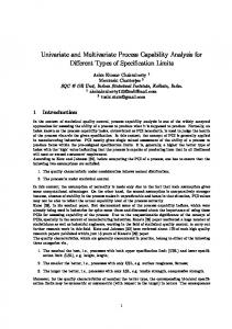
As γ → 0 the TM will converge to the mean in (14). Conversely, as γ → 0.50 then the TM will converge to the median. To demonstrate the use of the methodology above, presented in Figure 1 and Figure 2 are pdfs and cdfs from the Burr Type III and Type XII families, respectively. The values and graphs in these figures were obtained using various Mathematica [44] functions. More specifically, the values of c and k were obtained by solving equations (16) and (17) using the function FindRoot and the graphs of the pdfs and cdfs were determined using equations (9) and (10) and the function ParametricPlot. The modes were determined by evaluating 1 q(˜ u) = ((c − 1)/(ck + 1)) c for the solved values of c and k. The heights of the pdfs were subsequently obtained by solving for the values of u˜ that yielded the modes and then evaluating for the heights using 1/q 0 (˜ u) in (9). The values that yielded the probabilities of obtaining values of q(u) in the upper 5% of the tail regions were determined by evaluating the quantile functions in (5) and (6) for u = 0.95.
3
Fitting Burr Distributions to Data
Presented in Figure 3 are Burr Type XII pdfs superimposed on histograms of circumference measures (in centimeters) taken from the abdomen, chest, forearm, and knee of 252 adult males. Inspection of Figure 3 indicates that
µ = 0.2607 σ 2 = 0.0820 α1 = 1.0 α2 = −0.22 c = −97.7167 k = 0.0036
µ = 1.1244 σ 2 = 0.0292 α1 = 1.4 α2 = 5.2 c = −10.3939 k = 2.1775
Figure 1: Examples of c and k parameters for Type III distributions and their associated pdfs and cdfs. These distributions can also be empirically simulated by using the quantile function in Equation (5).
µ = 0.4186 σ 2 = 0.0772 α1 = 1.5 α2 = 4.5 c = 1.8149 k = 4.6909
µ = 0.0408 σ 2 = 0.0023 α1 = 2.75 α2 = 13 c = 0.9066 k = 20.0039
Figure 2: Examples of c and k parameters for Type XII distributions and their associated pdfs and cdfs. These distributions can also be empirically simulated by using the quantile function in Equation (6).
2215
Simulating Burr distributions
the Burr pdfs provide good approximations to the empirical data. We note that to fit the Burr pdfs to the data, the following transformation had to be imposed on the quantile function q(u) : (M σ − µS + Sq(u))/σ. The values of the means (M, µ) and standard deviations (S, σ) for the data and Burr pdfs are given in Figure 3. One way of determining how well a Burr pdf models a set of data is to compute a chi-square goodness of fit statistic. For example, listed in Table 1 below are the cumulative percentages and class intervals based on the Burr pdf for the chest data in Panel B of Figure 3. The asymptotic value of p = 0.290 indicates that the Burr pdf provides a good fit to the data. We note that the degrees of freedom for this test were computed as df = 5 = 10(class intervals) −4(parameter estimates) −1(sample size). Further, the Burr TMs given in Table 2 also indicate a good fit as the TMs are all within the 95% bootstrap confidence intervals based on the data. The confidence intervals are based on 25000 bootstrap samples. Cumulative % 5 10 15 30 50 70 85 90 95 100
Table 1: Observed and expected frequencies and chi-square test based on the Burr Type XII approximation to the chest data in Figure 3. Empirical Distribution 20% TM Abdomen 91.808 (91.030, 92.605) Chest 100.128 (99.546, 100.736) Forearm 28.699 (28.539, 28.845) Knee 38.491 (38.320, 38.637)
Burr TM 91.721 100.172 28.608 38.472
Table 2: Examples of Burr Type XII trimmed means (TMs). Each TM is based on a sample size of n = 152 and has a 95% bootstrap confidence interval enclosed in parentheses.
2216
T. C. Headrick, M. D. Pant, and Y. Sheng
M = 92.5560 S = 10.7831 α1 = 0.833419 α2 = 2.18074
µ = 0.793968 σ = 0.287478 c = 3.872133 k = 2.264652 (A) Abdomen
M = 100.824 S = 8.43048 α1 = 0.677492 α2 = 0.944087
µ = 0.559304 σ = 0.238712 c = 2.867086 k = 4.468442 (B) Chest
M = 28.6639 S = 2.02069 α1 = −0.218025 α2 = 0.825501
µ = 0.966818 σ = 0.0626464 c = 23.543917 k = 1.7765786 (C) Forearm)
M = 38.5905 S = 2.41180 α1 = 0.513663 α2 = 1.01687 Data
µ = 0.781809 σ = 0.239507 c = 4.446853 k = 2.576122
Burr Distribution
(D) Knee
Figure 3: Examples of Burr Type XII pdfs’ approximations to empirical data using measures of circumference (in centimeters) taken from n = 252 males. To fit the Burr distributions to the data the quantile functions q(u) were transformed as (M σ − µS + Sq(u))/σ.
2217
Simulating Burr distributions
4
Multivariate Data Generation
The family of Burr distributions we are considering can be extended from univariate to multivariate data generation by specifying T quantile functions q(u) of the form of either (5) or (6). Specifically, let Z1 , . . . , ZT denote standard normal variables where the distribution functions and bivariate density function associated with Zj and Zk are expressed as Z zj 1 Φ(zj ) = Pr{Zj ≤ zj } = (2π)− 2 exp{−u2j /2}duj (19) −∞ Z zk 1 (20) (2π)− 2 exp{−u2k /2}duk Φ(zk ) = Pr{Zk ≤ zk } = −∞
Using (19), it follows that a quantile function of the form of either (5) or (6) can be expressed as qj (Φ(zj )) because Φ(zj ) ∼ U [0, 1]. As such, the bivariate correlation between two standardized Burr distributions, denoted as xj (qj (Φ(zj ))) and xk (qk (Φ(zk ))), can be determined as Z
+∞
Z
+∞
ρxj (qj (Φ(zj ))),xk (qk (Φ(zk ))) =
xj (qj (Φ(zj )))xk (qk (Φ(zk )))fjk dzj dzk −∞
−∞
(22) for j 6= k and where the correlation ρzj zk in fjk is referred to as an intermediate correlation. Thus, the objective is to use equation (22) to solve for the values of the T (T − 1)/2 intermediate correlations ρzj zk such that T specified Burr distributions also have a specified correlation matrix. To generate multivariate Burr distributions, the process begins by assembling the solved intermediate correlations into a T ×T matrix and subsequently factoring this matrix (e.g., a Cholesky factorization). The results from the factorization are then used to produce standard normal deviates that are correlated at the intermediate levels as follows Z1 = a11 V1 Z2 = a12 V1 + a22 V2 .. . Zj = a1j V1 + a2j V2 + · · · + aij Vi + · · · + ajj Vj .. . ZT = a1T V1 + a2T V2 + · · · + aiT Vi + · · · + aT T VT
(23)
2218
T. C. Headrick, M. D. Pant, and Y. Sheng
where V1 , . . . , VT are independent standard normal random deviates and where aij represents the element in the i-th row and j-th column of the matrix associated with the Cholesky factorization. To generate the regular uniform deviates required for the quantile functions in (5) or (6), it is suggested that the following series expansion for the unit normal cdf [25] be used on the Zj in (23) as Φ(zj ) = .5+ϕ(zj ){zj +zj3 /3+zj5 /(3·5)+zj7 /(3·5·7)+zj9 /(3·5·7·9)+· · · } (24) where ϕ(zj )is the standard normal pdf and where the absolute error associated with (24) is less than 8 × 10⁻¹⁶ .
5
Numerical Example and Monte Carlo Simulation
Suppose we desire to generate correlated data associated with the following Type III and Type XII Burr distributions: (1) Panel A in Figure 1, (2) Panel A in Figure 2, and (3) Panel B in Figure 2 with the specified correlation matrix given in Table 3. Figure 4 gives Mathematica source code for numerically solving equation (22) for the three intermediate correlations that are given in Table 4. The results of a Cholesky factorization on the intermediate correlation matrix are given in Table 5. These results are then used in (23) to create Z1 , Z2 , and Z3 with the specified intermediate correlations.
Table 3: Specified correlations between three Burr distributions. See Figure 1, Panel A (q1 ); Figure 2, Panels A and B (q2 and q3 ).
Z1 Z2 Z3
Z1 1 0.504372 0.633945
Z2 Z3 0.504372 0.633945 1 0.736946 0.736946 1
Table 4: Solved intermediate correlations. To empirically demonstrate the procedure described above, the three selected Burr distributions in Figures 1 and 2 were simulated in accordance to
Simulating Burr distributions
2219
Figure 4: Mathematica code for computing the intermediate correlations listed in Table 4.
2220
T. C. Headrick, M. D. Pant, and Y. Sheng
a11 = 1 a12 = 0.504372 a13 = 0.633945 0 a22 = 0.863486 a23 = 0.483160 0 0 a33 = 0.603878 Table 5: Cholesky factorization on the intermediate correlations in Table 4. the specified correlation matrix in Table 3 using an algorithm coded in Fortran. The algorithm employed the use of subroutines UNI1 and NORMB1 [3] to generate pseudo-random uniform and standard normal deviates. Samples of size N = 10, 250, and 1000000 were drawn for each of the three selected distributions using the specified values of c and k given in Figures 1 and 2. For the samples of size N = 10 and 250 the empirical estimates of the correlations, α ˆ 1 and α ˆ 2 were computed using an averaging procedure across 25000 replications and are reported in Tables 6 and 7 along with their root mean squared errors (RMSEs). In terms of the samples of size N = 1000000, the statistics were computed directly on these single samples and are reported in Table 8. Inspection of Tables 6-8 indicates that the procedure produced excellent agreement between the empirical estimates and the specified parameters even for samples sizes as small as N = 10. q1 (Φ(Z1 )) q1 (Φ(Z1 )) 1 q2 (Φ(Z2 )) 0.504(0.359) q3 (Φ(Z3 )) 0.601(0.402)
Table 6: Estimated values of correlation, skew (ˆ α1 ), and kurtosis(ˆ α2 ) between three Burr distributions. See Figure 1, Panel A (q1 ); Figure 2, Panels A, B (q2 , q3 ). The estimates are based on 25,000 samples of size 10. The RMSEs are in parentheses.
Table 7: Estimated values of correlation, skew (ˆ α1 ), and kurtosis(ˆ α2 ) between three Burr distributions. See Figure 1, Panel A (q1 ); Figure 2, Panels A, B (q2 , q3 ). The estimates are based on 25,000 samples of size 250. The RMSEs are in parentheses.
Table 8: Estimated values of correlation, skew (ˆ α1 ), and kurtosis(ˆ α2 ) between three Burr distributions. See Figure 1, Panel A (q1 ); Figure 2, Panels A, B (q2 , q3 ). The estimates are based on single samples of size 1,000,000.
6
Comments
Monte Carlo and simulation techniques are widely used in statistical research. Since real-world data sets can often be radically non-normal, it is essential that statisticians have a variety of techniques available for univariate or multivariate non-normal data generation. As mentioned above, the Burr distributions have not been as popular as some other competing methods such as power method polynomials [7, 10, 13, 40] for simulating multivariate non-normal distributions. More specifically, Kotz et al. [22] noted “this [power] method does provide a way of generating bivariate non-normal random variables. Simple extensions of other univariate methods are not available yet” (p. 37). However, the extension of the Burr family of distributions from univariate to multivariate data generation, as presented above, makes this family a viable competitor to the power method because of its simplicity and ease of execution. Provided in Appendix A are values of the shape parameters c and k to assist the user of the methodology. These values can be used directly or can be used as initial guesses in an equation solver if other shape parameters are desired but not listed in the Tables. It is also important to point out that the solutions to the shape parameters are not unique and that the Type III and Type XII distributions are not mutually exclusive. For example, consider the Type III distribution depicted in Panel C of Figure 1. Given the values of α1 = 1.4 and α2 = 5.2 there also exists a Type XII distribution with these values of skew and kurtosis. The values of the shape parameters are c = 2.62418 and k = 2.57947.
2222
T. C. Headrick, M. D. Pant, and Y. Sheng
References [1] T. M. Beasley and B. D. Zumbo, Comparison of aligned Friedman rank and parametric methods for testing interactions in split-plot designs, Computational Statistics and Data Analysis, 42 (2003), 569-593. [2] P. J. Bickel and K. A. Docksum, Mathematical Statistics: Basic Ideas and Selected Topics, Prentice Hall, Englewood Cliffs, NJ, 1977. [3] R. C. Blair, Rangen, IBM, Boca Raton, FL, 1987. [4] I. W. Burr, Cumulative frequency functions, Annals of Mathematical Statistics, 13 (1942), 215-232. [5] I. W. Burr, Parameters for a general system of distributions to match a grid of α3 and α4 , Communications in Statistics, 2 (1973), 1-21. [6] A. S. Chernobai, F. J. Fabozzi, and S. T. Rachev, Operational Risk: A Guide to Basel II Capital Requirements, Models, and Analysis, John Wiley & Sons, New York, NY, 2007. [7] A. I. Fleishman, A method for simulating non-normal distributions, Psychometrika, 43 (1978), 521-532. [8] J. H. Gove, M. J. Ducey, W. B. Leak, and L. Zhang, Rotated sigmoid structures in managed uneven-aged northern hardwood stands: A look at the Burr Type III distribution, Forestry, 81 (2008), 21-36. [9] M. R. Harwell and R. C. Serlin, An experimental study of a proposed test of nonparametric analysis of covariance, Psychological Bulletin, 104 (1988), 268-281. [10] T. C. Headrick and S. S. Sawilowsky, Simulating correlated multivariate nonnormal distributions: Extending the Fleishman power method, Psychometrika, 64 (1999), 25-35. [11] T. C. Headrick and S. S. Sawilowsky, Properties of the rank transformation in factorial analysis of covariance, Communications in Statistics: Simulation and Computation, 29 (2000), 1059-1087. [12] T. C. Headrick and O. Rotou, An investigation of the rank transformation in multiple regression, Computational Statistics and Data Analysis, 38 (2001), 203-215. [13] T. C. Headrick, Fast fifth-order polynomial transforms for generating univariate and multivariate non-normal distributions, Computational Statistics and Data Analysis, 40 (2002), 685-711.
Simulating Burr distributions
2223
[14] T. C. Headrick and R. K. Kowalchuk, The power method transformation: Its probability density function, distribution function, and its further use for fitting data, Journal of Statistical Computation and Simulation, 77 (2007), 229-249. [15] T. C. Headrick, R. K. Kowalchuk, and Y. Sheng, Parametric probability densities and distribution functions for the Tukey g-and-h transformations and their use for fitting data, Applied Mathematical Sciences, 2 (2008), 449-462. [16] B. Hess, S. F. Olejnik, and C. J. Huberty, The efficacy of two improvementover-chance effect sizes for two-group univariate comparisons under variance heterogeneity and non-normality, Educational and Psychological Measurement, 61 (2001), 909-936. [17] J. R. Hipp and K. A. Bollen, Model fit in structural equation models with censored, ordinal, and dichotomous variables: Testing vanishing tetrads, Sociological Methodology, 33 (2003), 267-305. [18] D. C. Hoaglin, g-and-h distributions, In S. Kotz and N. L. Johnson (Eds.), Encyclopedia of Statistical Sciences (Vol. 3, pp. 298-301), John Wiley & Sons, New York, NY, 1983. [19] D. C. Hoaglin, Summarizing shape numerically: The g-and-h distributions, In D. C. Hoaglin, F. Mosteller, and J. W. Tukey (Eds.), Exploring Data Tables, Trends, and Shapes (pp. 461-513), John Wiley & Sons, New York, NY, 1985. [20] Z. A. Karian and E. J. Dudewicz, Fitting Statistical Distributions: The Generalized Lambda Distribution and Generalized Bootstrap Methods, Chapman & Hall, CRC, Boca Raton, FL, 2000. [21] M. G. Kendall and A. Stuart, The Advanced Theory of Statistics, vol. 1, 4th ed., MacMillan, New York, NY, 1977. [22] S. Kotz, N. Balakrishnan, and N. L. Johnson, Continuous Multivariate Distributions, vol. 1, 2nd ed., John Wiley & Sons, New York, NY, 2000. [23] R. K. Kowalchuk, H. J. Keselman, and J. Algina, Repeated measures interaction test with aligned ranks, Multivariate Behavioral Research, 38 (2003), 433-461. [24] S. R. Lindsay, G. R. Wood, and R. C. Woollons, Modelling the diameter distribution of forest stands using the Burr distribution, Journal of Applied Statistics, 43 (1996), 609-619. [25] G. Marsaglia, Evaluating the normal distribution, Journal of Statistical Software, 11 (2004), 1-10. [26] P. W. Mielke, Another family of distributions for describing and analyzing precipitation data, Journal of Applied Meteorology, 12 (1973), 275-280.
2224
T. C. Headrick, M. D. Pant, and Y. Sheng
[27] N. A. Mokhlis, Reliability of a stress-strength model with Burr type III distributions, Communications in Statistics: Theory and Methods, 34 (2005), 16431657. [28] S. Nadarajah and S. Kotz, q exponential is a Burr distribution, Physics Letters A, 359 (2006), 577-579. [29] S. F. Olejnik and J. Algina, An analysis of statistical power for parametric ancova and rank transform ancova, Communications in Statistics: Theory and Methods, 16 (1987), 1923-1949. [30] J. S. Ramberg and B. W. Schmeiser, An approximate method for generating symmetric random variables, Communications of the ACM, 15 (1972), 987-990. [31] J. S. Ramberg and B. W. Schmeiser, An approximate method for generating asymmetric random variables, Communications of the ACM, 17 (1974), 78-82. [32] J. S. Ramberg, E. J. Dudewicz, P. R. Tadikamalla, and E. F. Mykytka, A probability distribution and its uses in fitting data, Technometrics, 21 (1979), 201-214. [33] W. J. Reinartz, R. Echambadi, and W. W. Chin, Generating non-normal data for simulation of structural equation models using Mattson’s method, Multivariate Behavioral Research, 37 (2002), 227-244. [34] R. N. Rodriguez, A guide to the Burr type XII distributions, Biometrika, 64 (1977), 129-134. [35] B. J. Sherrick, P. Garcia, and V. Tirupattur, Recovering probabilistic information from option markets: Tests of distributional assumptions, Journal of Future Markets, 16 (1996), 545-560. [36] C. A. Stone, Empirical power and Type I error rates for an IRT fit statistic that considers the precision of ability estimates, Educational and Psychological Measurement, 63 (2000), 1059-1087. [37] P. R. Tadikamalla, A look at the Burr and related distributions, International Statistical Review, 48 (1980), 337-344. [38] H. A. Tejeda and B. K. Goodwin, Modeling crop prices through a Burr distribution and analysis of correlation between crop prices and yields using a copula method,Paper presented at the annual meeting of the Agricultural and Applied Economics Association, Orlando, FL, 2008. http://purl.umn.edu/6061. [39] J. W. Tukey, Modern techniques in data analysis, NSF sponsored regional research conference at Southern Massachusetts University, North Dartmouth, MA, 1977.
Simulating Burr distributions
2225
[40] C. D. Vale and V. A. Maurelli, Simulating multivariate non-normal distributions, Psychometrika, 48 (1983), 465-471. [41] M. Vorechovsky and D. Novak, Correlation control in small-sample Monte Carlo type simulations I: A simulated annealing approach, Probabilistic Engineering Mechanics, 24 (2009), 452-462. [42] D. R. Wingo, Maximum likelihood methods for fitting the burr type XII distribution to life test data, Biometrical Journal, 25 (1983), 77-84. [43] D. R. Wingo, Maximum likelihood methods for fitting the burr type XII distribution to multiply (progressively) censored life test data, Metrika, 40 (1993), 203-210. [44] S. Wolfram, The Mathematica Book, 5th ed., Wolfram Media, Champaign, IL, 2003.
2226
T. C. Headrick, M. D. Pant, and Y. Sheng
Appendix A. Tabled values of skew (α1 ), kurtosis (α2 ), and the shape parameters c and k for Burr Type III and Type XII distributions. The notation LB and UB indicate lower and upper boundary approximations of kurtosis. See Appendix B for these values.
Appendix B. Approximate values of the lower boundary (LB) and upper boundary (UB) of kurtosis for the Type III and Type XII distributions in the tables of Appendix A. LB(III) LB(XII) UB(XII) UB(III)