Dec 19, 2008 - Department's post-graduate students and affiliated post-doctoral researchers. .... elementary Akkadian and Sumerian under the tutelage of Simo Parpola, ...... 4 Included in the PDF version of this dissertation to be found at ...... mobile phones), but on the other hand, also fiction and non-fiction book-length.
Univariate, bivariate, and multivariate methods in corpus-based lexicography – a study of synonymy Antti Arppe
Academic dissertation to be publicly discussed, by due permission of the Faculty of Arts at the University of Helsinki in lecture room 13, on the 19th of December, 2008, at 12 o’clock.
University of Helsinki Department of General Linguistics P.O. Box 9 (Siltavuorenpenger 20 A) FI-00014 University of Helsinki Finland
PUBLICATIONS NO. 44 2008
Cover image: The tree seen from the researcher’s chamber on 6.5.2008 (Antti Arppe) ISSN 0355-7170 ISBN 978-952-10-5174-6 (paperback) ISBN 978-952-10-5175-3 (PDF) URL: http://ethesis.helsinki.fi/ Helsinki 2008 Helsinki University Print
To my father and mother Juhani and Raija Arppe
Abstract In this dissertation, I present an overall methodological framework for studying linguistic alternations, focusing specifically on lexical variation in denoting a single meaning, that is, synonymy. As the practical example, I employ the synonymous set of the four most common Finnish verbs denoting THINK, namely ajatella, miettiä, pohtia and harkita ‘think, reflect, ponder, consider’. As a continuation to previous work, I describe in considerable detail the extension of statistical methods from dichotomous linguistic settings (e.g., Gries 2003; Bresnan et al. 2007) to polytomous ones, that is, concerning more than two possible alternative outcomes. The applied statistical methods are arranged into a succession of stages with increasing complexity, proceeding from univariate via bivariate to multivariate techniques in the end. As the central multivariate method, I argue for the use of polytomous logistic regression and demonstrate its practical implementation to the studied phenomenon, thus extending the work by Bresnan et al. (2007), who applied simple (binary) logistic regression to a dichotomous structural alternation in English. The results of the various statistical analyses confirm that a wide range of contextual features across different categories are indeed associated with the use and selection of the selected think lexemes; however, a substantial part of these features are not exemplified in current Finnish lexicographical descriptions. The multivariate analysis results indicate that the semantic classifications of syntactic argument types are on the average the most distinctive feature category, followed by overall semantic characterizations of the verb chains, and then syntactic argument types alone, with morphological features pertaining to the verb chain and extra-linguistic features relegated to the last position. In terms of overall performance of the multivariate analysis and modeling, the prediction accuracy seems to reach a ceiling at a Recall rate of roughly two-thirds of the sentences in the research corpus. The analysis of these results suggests a limit to what can be explained and determined within the immediate sentential context and applying the conventional descriptive and analytical apparatus based on currently available linguistic theories and models. The results also support Bresnan’s (2007) and others’ (e.g., Bod et al. 2003) probabilistic view of the relationship between linguistic usage and the underlying linguistic system, in which only a minority of linguistic choices are categorical, given the known context – represented as a feature cluster – that can be analytically grasped and identified. Instead, most contexts exhibit degrees of variation as to their outcomes, resulting in proportionate choices over longer stretches of usage in texts or speech.
v
Preface and acknowledgments
ud mu-e-ši-zal a-na-am3 šu mu-da-ti ‘The time passed, and what did you gain?’1 2
nam-sag9-ga kaš-a nam-hul kaskal-la ‘The good thing – it is the beer, the bad thing – it is the journey.’3 This dissertation is essentially the product of a decade-long sequence of innumerable discussions, in which my supervisors, colleagues, friends, and family have imparted ideas and insights that have edged my research further. Not only have these discussions taken place during supervision and consultation sessions proper, but they have chanced to happen while crossing a street, in informal meetings in the University’s corridors, by the copy-machine or printer at the Department, over the phone or via e-mail, during the short question-and-answer sessions or the longer chitchat that follows at academic conferences, workshops, and seminars, or even through the age-old medium for the exchange of scientific ideas through written books or articles. All too often, I have not fully appreciated such ideas when they have first been proffered to me – probably because I was not yet ready to understand them yet – and sometimes the true value of many a suggestion has dawned on me only years afterwards. In all likelihood, my partners in these discussions may not have realized themselves what – in retrospect – crystal-clear one-liners they have uttered or written concerning one aspect or another relevant to my research process. Nonetheless, these giveaway reflections are what I can now see to form the backbone of this written work. Although this study is thus fundamentally the result of applying an ensemble of many borrowed ideas, my own contribution – and therefore also nobody else’s responsibility but mine – is the complex whole that they constitute and the overall interpretation that is conveyed.
1
Electronic Text Corpus of Sumerian Literature: Proverbs, Collection 3: 3.157 (Black et al. 19982008). 2 CompositeCuneiform signs by Tinney and Everson (2004-2007). 3 Electronic Text Corpus of Sumerian Literature: Proverbs, Collection 7: 7.98 (Black et al. 1998-2006).
vi
I am deeply grateful to my four official supervisors, Fred Karlsson, Lauri Carlson, Urho Määttä, and Juhani Järvikivi, for each guiding in their own characteristic manner this work further towards its final conclusion. Fred Karlsson saw promise in my early, quite sketchy research plan concerning synonymy, accepting me, as the academic immigrant from engineering that I was, into the field of linguistics as a post-graduate student, as well as tipping me off about my first research funding in the GILTA project. Fred’s persistent insistence on focusing on the final goal, however uncomfortable I found the issue at times, was instrumental in getting this dissertation finished. Lauri Carlson was a wizard in articulating what I was not yet able to, seeing where my thinking was taking me before I knew it myself, and crystallizing these into simple comments or questions that connected my tiny, seemingly isolated island of research into the grander scheme of things within the linguistic discipline. During the final writing process of this text, Lauri pored through diligently each chunk as I succeeded in churning them out, providing me the assurance that I remained on the right track. Urho Määttä always had ample time and interest to discuss the most general ramifications and connections of my work and to delve deep into what language as an object of study and linguistics as a discipline were fundamentally about. At the same time, Urho assisted me in contenting myself first with only one, seemingly small, part of my original research plan, and then mastering that portion as comprehensively as possible. Juhani Järvikivi’s expertise in psycholinguistic experimentation was the component that I did not know was missing until I stumbled onto it, and which was to open my eyes to what my research in linguistics could on the long term concern. Co-authoring two journal articles together with Juhani introduced me to what academic discourse at the international level is really about, and this co-operation also allowed me to sketch out the general, multimethodological backdrop which this considerably more tightly focused work serves. I am also indebted to Martti Vainio, who acted as my fifth supervisor in all but name. It was Martti who realized that logistic regression might be the very statistical method that could bring some order to my jungle of linguistic features, and he neither hesitated nor spared his time in working out with me a solution to applying this technique to my multiple-outcome setting and getting me started with R. I also appreciate Martti’s iconoclastic attitude in the many intensive but free-wheeling discussions we have had concerning a wide array of topics ranging from the current central questions in linguistics and other sciences to international politics, in which we have not been troubled by the passing of time. Furthermore, I am grateful to Kimmo Koskenniemi for all the support and sincere attention he has shown to the progress of my research work. Thanks to Kimmo, I originally wound up working in the mid-to-late 1990s at Lingsoft, a small Finnish language technology company, where one of the software development projects I was involved in, namely inflecting thesauri, would lead me to discover the kernel of this dissertation. In particular, I want to thank Kimmo for inviting me on several occasions
vii
to speak in the language technology seminar in order to sort out the state of my research and rediscover its red thread, when I was in danger of losing my way. At the Department of General Linguistics, I have appreciated the collegial and informal atmosphere, which has allowed me to benefit from the experience of the research and teaching staff representing three closely related but distinct subjects. I am thankful for the patient coaching and support by Jan-Ola Östman and Kari K. Pitkänen when I was still primarily a full-time novice in the field. Moreover, I have fond memories of the late Orvokki Heinämäki, who taught some of the very first courses in general linguistics that I took in the early 1990s. Most importantly, I have also had the excellent opportunity to broaden my understanding of linguistics through encountering the extraordinarily diverse kaleidoscope research topics pursued by the Department’s post-graduate students and affiliated post-doctoral researchers. Among many others, I am happy to have had a lively interchange with Matti Miestamo, in which he has convincingly argued for the importance of typological perspective in linguistics. In particular, I want to thank Matti for providing me with comments in this respect on the Introduction and Discussion of this text, and for the extra-curricular discussions we have had as fellow Kallio linguists. I am very grateful to both of my preliminary examiners, R. Harald Baayen (University of Alberta) and Stefan Th. Gries (University of California, Santa Barbara), for their constructive criticism with respect to the current text and their encouraging suggestions to continue developing its themes further. In fact, when I had first made the acquaintance of both my examiners, on separate occasions just around the beginning of this millennium, they had each given me tips that I did not heed at the time, but which advice I later realized to contain two cornerstones of this dissertation. Harald Baayen was the first person to recommend to me that I get acquainted with the R statistical programming environment, which became the workhorse for all the statistical analysis in my work, while Stefan Th. Gries’ own doctoral dissertation already contained the general tripartite methodological setup that I was to find wellsuited to bring structure also to my work. In addition, there are a great number of scholars both in Finland and abroad with whom I have had the opportunity, privilege and pleasure of collaborating or exchanging ideas, opinions, and assistance over the many years, not always only concerning linguistics but also the practical everyday challenges of leading the life a young researcher. These people whom I wish to recognize are (in alphabetical order): Daniel Aalto, Tiina Arppe, Lili Aunimo, Juhani Birn, Pia Brandt, Joan Bresnan, Andrew Chesterman, Pernilla Danielsson, Dagmar Divjak, Antonina Durfee, NilsErik Enkvist, Stefan Evert, Marja Etelämäki, Sam Featherston, Dylan Glynn, Stefan Grondelaers, Mickel Grönroos, Erja Hannula, Tarja Riitta Heinonen, Irmeli Helin, Kris Heylen, Suvi Honkanen, Timo Honkela, Silja Huttunen, Esa Itkonen, Jarmo H. Jantunen, Eriika Johansson, Kristiina Jokinen, Timo Järvinen, Panu Kalliokoski, Irina Kauhanen, Tapani Kelomäki, Harri Kettunen, Tarja Knuuttila, Leena Kolehmainen, Lari Kotilainen, Ville Laakso, Krista Lagus, Ritva Laury, Jaakko Leino, Pentti Leino, Yrjö Leino, Krister Lindén, Mikko Lounela, Aapo Länsiluoto, Laura Löfberg, Anke Lüdeling, Annu Marttila, Matti Miestamo, Manne Miettinen, Sjur Nørstebø Moshagen, Jussi Niemi, Otto Nieminen, Urpo Nikanne, Alexandre Nikolaev, Torbjørn Nordgård, Elina Nurmi, Martti Nyman, Seppo Nyrkkö, Krista Ojutkangas, Jussi Pakkasvirta, Heikki Patomäki, Pertti Palo, Santeri Palviainen, Simo Parpola,
viii
Marja Peltomaa, Kaarina Pitkänen, Marja Pälsi, Michaela Pörn, Jarno Raukko, Timo Riiho, Jouni Rostila, Jack Rueter, Janne Saarikivi, Gabriel Sandu, Dirk Speelman, Kaius Sinnemäki, Pirkko Suihkonen, Mickael Suominen, Antti Suni, Gert De Sutter, Pasi Tapanainen, Lauri Tarkkonen, Jarmo Toivonen, Trond Trosterud, Jarno Tuimala, José Tummers, Tuuli Tuominen, Ulla Vanhatalo, Johanna Vaattovaara, Kari T. Vasko, Kimmo Vehkalahti, Marja Vierros, Simo Vihjanen, Liisa Vilkki, Maria Vilkuna, Laura Visapää, Mari Voipio, Atro Voutilainen, Tytti Voutilainen, Jarmo Välikangas, Fredrik Westerlund, Caroline Willners, Malene Würtz, Anssi Yli-Jyrä, and Jussi Ylikoski. From my time at Lingsoft, I am especially grateful to Juhani Birn for his witty insight and seasoned experience in interpreting the unexpected behavior of inflecting thesauri. Likewise, I appreciate the initial effort that Mari Voipio and Malene Würtz made to put our finger on what the oddities exactly were and what they might generally entail. Moreover, I truly enjoyed the many manifold times that we managed to drift over to discussing linguistic topics together with many of the company’s employees in the late 1990s. For the first three years of my postgraduate studies, I participated in and received funding through the GILTA project, led by Ari Visa (Tampere University of Technology), Hannu Vanharanta (Tampere University of Technology), and Barbro Back (Åbo Akademi University). I appreciate greatly the wide latitude that I was allowed within this cross-disciplinary project, permitting me to pursue my purely linguistic research interests at the same time. Especially glad I am that we succeeded in tying most of the different strands of research together in one major joint article, in which the individual contributions of Tomas Eklund (Åbo Akademi University) and Camilla Magnusson played a central role. Although Camilla started out as my research assistant in the GILTA project, she soon became an independent-minded researcher in her own right, and I am grateful to her for questioning some certainties that I held. Already in 1999, I had been invited by Anu Airola and Hanna Westerlund to join an informal post-graduate discussion group, which soon extended to include also Jussi Piitulainen. I am thankful to Anu, Hanna, and Jussi for all the mutual assistance and instruction that was of great help to me in trying to make sense – both to myself and the others – of what various central theoretical concepts meant or could connote. During 2002-2003, this evolved into the Suomenlinna circle of linguists, also known as TR-9, formed by Urho Määttä, Anu Airola, Juhani Järvikivi, Camilla Magnusson, Jussi Piitulainen, Reetta Konstenius, Martti Vainio, Hanna Westerlund, and myself. TR-9 gave me an inspiring glimpse of the satisfying intellectual interchange that can be achieved when linguists with diverse backgrounds and complementary skills work together rather than alone. In particular, I still remember clearly Reetta’s insistence on the rigorous formation of hypotheses and firm argumentation while conducting linguistic research. Beginning in 2003, I had the privilege of being accepted into LANGNET, the Finnish Graduate School in Language Studies, within which I received full funding for the first four years, followed by an additional year as a self-financed fellow. I have come to consider many of my postgraduate colleagues within the LANGNET graduate school, as well as recent doctors, to form a unique peer group that is best positioned to
ix
wholly understand the many conflicting demands and to provide support in the difficult challenges that young researchers face these days. Many of these originally primarily professional colleagues I now consider also my friends. During my research process and the writing of this dissertation text, I have had the privilege of tapping into the expert knowledge of some of the foremost and upcoming specialists in Finland outside my own restricted field. At the postgraduate seminars organized by the Department of Finnish language and literature, which I had the pleasure of attending twice, I was happy to receive from Pentti Leino both commonsense and worthwhile feedback from the Fennistic perspective on interpreting quantitative results arising from my statistically-oriented line of research. When I have needed guidance concerning the etymological roots of the THINK verbs that I study or help with rarer infinitival or other infrequent forms in Finnish, I have had the opportunity to consult Jussi Ylikoski’s unfailing store of knowledge. I have also been able to indulge in my interest in writing systems by studying the cuneiform script, elementary Akkadian and Sumerian under the tutelage of Simo Parpola, and Maya hieroglyphs under the guidance of Harri Kettunen. These studies have provided me a truly welcome and worthwhile, culturally and historically rich counterpart and relaxation to my otherwise quite numeric study. Moreover, I wish to thank Harri for his peer-support during some trying times in my research process, which I hope to be able to reciprocate. In the linguistic analysis of my research data, I was fortunate enough to have for several months two research assistants, Marjaana Välisalo and Paula Sirjola, to produce comparative analyses for parts of the data. I can only admire the thorough inquisition to which I was subjected concerning my principles of classification, which certainly became more uniform and explicit in the process, and I commend them both for the diligence in applying these principles in their own analysis of the data. In the numerous statistical analyses undertaken throughout my research process, I am grateful to Daniel Aalto (Helsinki University of Technology), Pertti Palo (Helsinki University of Technology), Lauri Tarkkonen, Kimmo Vehkalahti, Seppo Nyrkkö, and Kari T. Vasko (CSC – IT Center for Science) for the invaluable advice that I have received countless times. Especially indebted I am to Daniel Aalto, who inspected Sections 3-4 describing the array of statistical methods applied in this study, although any possible faults and mistakes naturally remain mine alone. I also want to thank Seppo Nyrkkö for his assistance in getting R to work properly with the Finnish character set on my portable Macintosh, and Jarno Tuimala and Yrjö Leino (both of CSC – IT Center for Science) for providing me all the programming and other assistance necessary for the parallel computations that I undertook on CSC’s brandnew murska supercluster system. Likewise, I owe many thanks to the administrative and support staff at our Department, in the Faculty of Arts, and in the LANGNET graduate school for keeping the paperwork and infrastructure running smoothly, so that I and other researchers could mostly concentrate on academic matters. Especially, I want to mention Johanna Ratia, Anders Enkvist, Jaakko Leino, Ulla Vanhatalo, Hanna Westerlund, Tiina Keisanen, Miroslav Lehecka, Jussi Luukka, and Kristiina Norlamo for doing their utmost to facilitate my research work, not to forget Kirsti Kamppuri, Ardy Pitré, and others who no longer work in the academic world.
x
In the final drive to get this text ready for publication and public defense, I am glad that I could count on the efforts of Leila Virtanen, Jack Rueter, Graham Wilcock, in order to ensure that the quality of the language matched up to the content of the text. In particular, I am indebted to Jack Rueter and Leila Virtanen for their willingness to help me iron out the last stylistic wrinkles at very short notice. My research has been financially supported for seven years within the GILTA project (funded by TEKES, the National Technology Agency of Finland within its USIX technology program: 40943/99) and the LANGNET graduate school (funded by the Finnish Ministry of Education), for which I am most grateful. In addition, I wish to thank the Chancellor of the University of Helsinki for several travel grants. Moreover, I am thankful to Juhani Reiman and Simo Vihjanen at Lingsoft for making generous use of my prior experience and linguistic knowledge at a remunerative rate to supplement my income. Furthermore, I also appreciate the many discussions concerning the philosophy of language and its study that I have had with Simo Vihjanen. I am also thankful to Pertti Jarla, Punishment Pictures and PIB for permission to use a strip from Fingerpori. Finally, though a level of seclusion and social fasting seems to facilitate the conclusion of a doctoral dissertation, it would be hard to follow through with the entire post-graduate project solely within an academic bubble, with no connections to the rest of the world. In this respect, I am deeply grateful for the unwavering encouragement and patient understanding by my old and newer friends from Kulosaari, Helsinki University of Technology, TKY, Prodeko, the Polytech Choir, Teekkarispeksi, Kårspex, Spock’s HUT, Aspekti, SKY – Linguistic Association of Finland, Flemarin Piikki, Pikku-Vallila, FC Heinähattu, Rytmi, and whatnot. Special mentions are awarded to the Antti Club for carrying on our culinary circuit, and Ryhmä Rämä ‘Team Daredevil’ for keeping in touch despite our distributed locations around the globe. I also thank my two godchildren, Juuso Rantanen and Otto Jalas, for the instant getaways I have always had in their company, providing an excellent antidote when I had lost myself too deep into scientific thought. Last but not least, I wish to express my profound gratitude and appreciation to my immediate family for all the love, care, and concrete support that they have provided me throughout this longer-than-originally-anticipated and demanding process. To mention only a few details, I am thankful to my brother Tuomas Arppe for furnishing me a practical field stretcher to my workroom so that I need not take an afternoon nap on the cold floor, and to my sister Helena Arppe for helping me arrange the stylistic review of my dissertation text. What is more, I am immensely indebted to my father and mother, Juhani and Raija Arppe, for understanding and backing whatever decisions I have taken in my life, even supporting the very final phase financially, and in encouraging me to boldly go for my own thing. Antti Arppe Helsinki December 2008
xi
Table of Contents 1 1.1 1.2 1.3 1.4
Introduction.......................................................................................................... 1 The empirical study of language and the role of corpora .................................... 1 Synonymy and semantic similarity...................................................................... 7 Theoretical premises and assumptions in this study .......................................... 13 The goals of this study and its structure............................................................. 13
2 Data and its linguistic analysis........................................................................... 17 2.1 Selection of the studied synonyms..................................................................... 17 2.1.1 Background in prior studies ............................................................................... 17 2.1.2 Screening out the interrelationships of COGNITION lexemes by their dictionary definitions ......................................................................................... 20 2.1.3 Clustering the COGNITION lexemes by statistical means .................................... 23 2.1.4 Extracting frequencies for THINK lexemes......................................................... 25 2.2 Selection of the contextual features and their application in the analysis............................................................................................................... 28 2.3 Present descriptions of the studied THINK synonyms......................................... 33 2.3.1 THINK lexemes in Pajunen’s Argumenttirakenne............................................... 33 2.3.2 THINK lexemes in Suomen kielen perussanakirja and Nykysuomen sanakirja ............................................................................................................ 36 2.3.3 The etymological origins of the selected THINK lexemes................................... 48 2.4 The compilation of the research corpus and its general description .................. 50 2.4.1 General criteria................................................................................................... 50 2.4.2 Main characteristics of the final selected research corpus................................. 52 2.4.3 Coverage of contextual features in the research corpus..................................... 55 2.4.4 Representativeness, replicability, reliability, and validity ................................. 66 2.5 Preparation of the corpus for statistical analysis................................................ 69 3 Selection and implementation of statistical methods......................................... 71 3.1 Practical implementation of the employed statistical methods.......................... 71 3.2 Univariate methods ............................................................................................ 73 3.2.1 Homogeneity or heterogeneity of the distribution – independence or dependence?....................................................................................................... 75 3.2.2 Measures of association ..................................................................................... 86 3.2.3 Grouped univariate analysis for a set of related contextual features ................. 94 3.3 Bivariate methods ............................................................................................ 105 3.3.1 General considerations..................................................................................... 105 3.3.2 Pairwise associations of individual features .................................................... 106 3.3.3 Pairwise comparisons of two sets of related features ...................................... 108 3.4 Multivariate methods ....................................................................................... 113 3.4.1 Logistic regression analysis with nominal outcomes and variables ................ 113 3.4.2 Selection of variables in multivariate logistic regression ................................ 116 3.4.3 Alternative heuristics of multinomial regression analysis ............................... 119 3.4.4 Evaluating the polytomous logistic regression models and their performance ..................................................................................................... 126 3.4.5 A detailed example of a (binary) logistic regression model ............................ 139 3.4.6 Other possible or relevant multivariate methods ............................................. 150
xii
4 Univariate and bivariate results ....................................................................... 153 4.1 Univariate analyses .......................................................................................... 153 4.1.1 General results ................................................................................................. 153 4.1.2 Characterizations of the studied THINK lexemes on the basis of the univariate results .............................................................................................. 160 4.1.3 Comparison of the univariate results with existing lexicographical descriptions ...................................................................................................... 163 4.2 Bivariate correlations and comparisons ........................................................... 170 4.2.1 Pairwise correlations of singular features ........................................................ 170 4.2.2 Pairwise associations of grouped features ....................................................... 182 5 5.1 5.2
5.6
Multivariate analyses ....................................................................................... 187 Selection of variables....................................................................................... 187 Comparisons of the descriptive and predictive capabilities of the different heuristics and models ........................................................................ 198 Comparing the various heuristics with respect to the full model..................... 198 The lexeme-wise breakdown of the prediction results .................................... 201 Comparing the performance of models with different levels of complexity........................................................................................................ 204 Relative lexeme-wise weights of feature categories and individual features............................................................................................................. 209 Overview of the lexeme-specific feature-wise odds ........................................ 209 Lexeme-wise analysis of the estimated odds ................................................... 212 Feature-wise analysis of the estimated odds.................................................... 213 Comparison with the univariate results............................................................ 216 Comparison with descriptions in current dictionaries ..................................... 217 Assessing the robustness of the effects............................................................ 220 Simple bootstrap and writer-cluster resampling .............................................. 220 Assessing the effect of incorporating extralinguistic features ......................... 224 Probability estimates of the studied lexemes in the original data.................... 228 Overall assessment of lexeme-wise probability estimates............................... 228 Profiles of instance-wise distributions of the lexeme-wise probability estimates........................................................................................................... 237 “Wrong” choices in terms of lexeme-wise estimated probabilities ................. 239 Contexts with lexeme-wise equal probability estimates – examples of synonymy? ....................................................................................................... 241 Deriving general scenarios of probability distribution profiles with clustering.......................................................................................................... 246 New descriptions of the studied synonyms...................................................... 248
6 6.1 6.2 6.3
Discussion ........................................................................................................ 253 Synonymy and its study and description in light of the results ....................... 253 Hypotheses for experimentation on the basis of the results............................. 259 Suggestions for other further research and analyses........................................ 261
7
Conclusions...................................................................................................... 265
5.2.1 5.2.2 5.2.3 5.3 5.3.1 5.3.2 5.3.3 5.3.4 5.3.5 5.4 5.4.1 5.4.2 5.5 5.5.1 5.5.2 5.5.3 5.5.4 5.5.5
Corpora....................................................................................................................... 268 References................................................................................................................... 269
xiii
Appendices4 Appendix A. Evaluation of the interchangeability of selected THINK lexemes among the example sentences provided in PS (Haarala et al. 1997) ............... 288 Appendix B. Details concerning the selection of the studied THINK lexemes ............ 289 Appendix C. Description of the various stages and levels in the linguistic annotation process and of the contextual features applied therein .................. 317 Appendix D. List of morphological, surface-syntactic and functional syntactic features used in the linguistic analysis............................................................. 350 Appendix E. Figures and selected details concerning the performance of the FI-FDG parser and the consistency of the manual annotation on the research data..................................................................................................... 384 Appendix F. Linguistic analyses of the lexical entries of the studied THINK lexemes in Suomen kielen perussanakirja (PS) and Nykysuomen sanakirja (NS).................................................................................................. 422 Appendix G. Lexeme-wise aggregates of the linguistic analyses of the lexical entries for the studied THINK lexemes, integrating the contents of both Perussanakirja and Nykysuomen sanakirja ..................................................... 436 Appendix H. Posited etymologies of selected THINK lexemes ................................... 442 Appendix I. An in-depth discussion of the text types incorporated in the sources selected into the research corpus, as well as a detailed description of the compilation and resultant characteristics and composition of this corpus ............................................................................... 444 Appendix J. Frequency data concerning the selected sources for the research corpus, namely, Helsingin Sanomat (1995) and SFNET (2002-2003), plus an original data sample from Helsingin Sanomat .................................... 466 Appendix K. A Zipfian alternative for scrutinizing expected distributions of features among the studied THINK lexemes...................................................... 478 Appendix L. An in-depth discussion of the conceptual foundations and associated parameters for the measures of association presented in Section 3.1.2..................................................................................................... 488 Appendix M. Interaction of medium with person/number features, semantic types of agents, and semantic and structural types of patients, studied in a dichotomous model pitting ajatella against the other three THINK lexemes ............................................................................................................ 499 Appendix N. A full-depth presentation and discussion of selected univariate results ............................................................................................................... 502 Appendix O. Some general results concerning the Zipfian scrutiny of the distributions of the studied features among the selected THINK lexemes......... 542 Appendix P. Complete univariate results ................................................................... 544 Appendix Q. Complete bivariate results..................................................................... 560 Appendix R. Complete multivariate variable sets and results .................................... 568 Appendix S. Brief descriptions of the main R functions applied throughout this dissertation ................................................................................................ 597
4
Included in the PDF version of this dissertation to be found at URL: http://ethesis.helsinki.fi/
xiv
1
Introduction
1.1
The empirical study of language and the role of corpora
Human language is a multimodal phenomenon, involving physical, biological and physiological, psychological and cognitive, as well as social dimensions. Firstly, language is physical through the sound waves, gestures, written symbols, and electronic forms with which it is communicated by one language user to another, and which are the manifestations of language that we can externally perceive and observe easily. Secondly, language is biological and physiological with respect to the organs and senses that produce, receive, and process the physical manifestations of language, including the vocal tract, ears and hearing, eyes and sight, hands, and in some rarer cases also touch, and most importantly, the brain. Thirdly, language is psychological and cognitive in that its externally observable manifestations are linked with a psychological representation in the human cognitive system, yielding the Saussurean dichotomy between form and meaning. Fourthly, language is a social phenomenon: such meaning – and even the associated form – is constructed through and as a part of the collective activity and interpersonal communication of human beings; with no communicative or other socially shared functions language and its manifestations are meaningless. Therefore, it is surprising that the study of language, linguistics, has, at least in the second half of the twentieth century seen a predilection for methodological monism (cf. Hacking 1996: 65-66). Firstly, the influential generative school (Chomsky 1965: 4, 65, 201) in its various incarnations has traditionally deemed language use, as manifested in, for example, corpora, as deficient and erroneous evidence about language as a system and the rules and regularities that it consists of, and thus an unreliable source of evidence in the study of language. The result of this reasoning has been the elevation of introspection, prototypically by the linguist himself with respect to his own intuitions about a linguistic phenomenon, as the primary type of linguistic evidence. The associated marginalization of corpora by generativism, however, has not been as uniformly categorical as is generally assumed (Karlsson, forthcoming 2008). Nevertheless, from the perspective of science studies, this in effect methodological exclusiveness by generativists – Noam Chomsky in particular – has been criticized as simplistic, as though it were implying that there was only one proper “style” of conducting modern science, that is, hypothetical modeling, when there are in fact many appropriate methods (Hacking 1996: 64-66, see also Crombie 1981: 284 for the general typology of scientific “styles”5); similar critical arguments have also been voiced within linguistics (Chafe 1992: 96; Wasow and Arnold 2005: 1484). Furthermore, within the generative school itself as in others, intuition and introspection, specifically as undertaken by the researchers themselves, have been demonstrated to be unreliable and inconsistent as a method (e.g., Schütze 1996; Bard et al. 1996; Sampson 2001, 2005; Gries 2002; Wasow and Arnold 2005; Featherston 5
The varieties of “styles” of science according to Crombie (1981: 284) are “1) simple postulation established in the mathematical sciences, 2) the experimental exploration and measure of more complex observable relations, 3) the hypothetical construction of analogical models, 4) the ordering of variety by comparison and taxonomy, 5) the statistical analysis of the regularities of populations and the calculus of probabilities, and 6) the historical derivation of development. The first three of these methods concern essentially the science of individual regularities, and the second three the science of the regularities of populations ordered in space and time.” [numbering added by A.A.]
1
20076). Some of these critics even appear prepared to go as far as discrediting any type of linguistic research method building upon intuition, such as elicitation or experimentation, a view most strongly vocalized by Sampson (2001: 129; 2005: 17; 2007a: 15; 2007b: 119). In the late twentieth century, the natural use of language, collected and compiled as corpora, has predominantly been presented as the empirical solution to the inadequacy of introspection. This development has been particularly strengthened by the increasing availability of texts in electronic form, attributable firstly to the extremely successful diffusion of the personal computer, and, more recently, by the rapid dissemination of the Internet and the accelerating expansion of its content. However, proponents of this source of evidence have also been inclined to methodological preferentialism if not outright monism, as Chafe (1992: 96) so aptly puts it. At the least, it is fair to say that many language researchers who identify themselves as “corpus linguists” would elevate corpora as the most preferred or the most precise source of linguistic evidence (e.g., Leech et al. 1994; Sampson 2001, 2005; Gries 2002: 38); some would even go as far as to rank recordings of spoken language – representing the most natural and basic mode of linguistic behavior – first in a hierarchy of linguistic data (Sampson 2001: 7-10). However, even corpus linguists are willing to admit that corpora cannot always provide a satisfactory or complete answer to all linguistically interesting or important research questions. First of all, it is difficult – if not impossible – to study rarer linguistic phenomena on the basis of corpora alone, as it is hard to distinguish such infrequent items from genuine errors, slips of the tongue, or effects of linguistic/cognitive disorders in production, or yet unestablished new forms or constructions resulting from linguistic change in the making (e.g., Sampson 2007a: 14). What is more, the inability of corpora, being fundamentally samples of language use, to produce direct negative evidence has also traditionally been presented as a limitation to their status as linguistic evidence. In other words, the absence of a given linguistic phenomenon in some corpus, while it may be indicative of the rarity of this phenomenon and thus a low expected probability of occurrence, cannot be taken as definitive, conclusive evidence that the phenomenon in question would not with certainty be a proper and acceptable linguistic structure (e.g., Atkins and Levin 1995: 87, 108; Hanks 1996: 78).7 Nevertheless, the issue of negative evidence is a problematic one for any empirical science. Finally, there is an ongoing discussion concerning the representativeness of corpora and how to improve this state of affairs, 6
It is peculiar to note that in Featherston’s (2007: 271) judgment the original criticisms concerning self-introspection as evidence by Schütze and others, presented already more than a decade ago, have not yet been fully accepted among a significant number of the generative linguists; apparently “old habits die hard.” 7 This has been countered with the argument that natural sciences, such as physics, typically presented as the model to be followed in linguistics and other human-oriented, social sciences in order to be considered “proper”, “hard” sciences, generally do not require negative evidence. For instance, the fact that we always see bricks falling down and never levitating upwards (by themselves) does allow us to conclude both that (a) gravity causes objects to be attracted towards each other, as well as that (b) gravity does not cause objects to be repelled away from each other, unless some other force is at play; though one could logically counter that we may have missed observing (b) to happen somewhere in the universe (adapted from a posting by Geoffrey Sampson 4.1.2008 to the Corpora mailing list). This view of the natural sciences as not using any negative evidence at all has been disputed by, e.g., John Goldsmith (posting 3.1.2008 to the same list).
2
that is, what exactly constitutes the entire population of different types of language usage events that corpora currently represent, and in the future could and should incorporate, and what the proportions of these types sampled into corpora as well as their overall sizes should be (e.g., Clear 1992; Biber 1993; Váradi 2001; Kilgarriff and Grefenstette 2003: 336, 40-341; Leech 2007: 132). Any foreseeable developments, however, do not eliminate the fact that even an extremely large and comprehensive – and thus a very representative corpus or set of corpora – would still be representative of only one, even if central, aspect of linguistic behavior, namely, usage, with a bias towards production. In fact, the range of different types of phenomena that can be considered part of or relevant to linguistic behavior, and which thus can also provide us with linguistic evidence, is quite diverse (e.g., Penke and Rosenbach 2004b: 485). Besides introspection or corpora made up of written or spoken language, we can also solicit judgements by (typically) native speakers concerning the grammaticality or acceptability of a linguistic form or structure; this is at its core in fact more commonplace as a linguistic activity than one might initially expect, since we encounter or engage in it all the time when we teach or learn a language, or when we attempt to guess the dialect of a native speaker or the underlying mother tongue of a second-language learner. Such elicitation has long been established as the central method in creating descriptions for previously (in scientific terms) unstudied languages, often in practice from scratch, within the domain of field linguistics. In addition, we can use linguistic errors and slips of the tongue by “normal” language users, or errors committed by language learners or people with linguistic/cognitive disorders of various sorts. Furthermore, we can study reaction times to visual or oral linguistic stimuli, the speed and progress of reading and the associated eyemovements, thus linking linguistics to the methodology of psychology. Or we can use neuroimaging to study how various parts of the brain are activated in conjunction with linguistic stimuli and tasks, linking linguistics to biology and cognitive science. On closer inspection, we see that these other sources of evidence are customarily found outside the confines of theoretical “core” linguistics “proper” as it has been largely conceived in the second half of the twentieth century, in its many “hyphenated” subfields. Penke and Rosenbach (2004b: 485-491) attempt to give some structure to this methodological and evidential multitude by providing a tentative general classification along three dimensions. The first of these concerns quantitative vs. qualitative focus, that is whether we are interested in how many times a linguistic phenomenon occurs (in comparison to others), or in the dichotomy whether it occurs at least once or not at all. The second dimension contrasts direct vs. indirect evidence, distinguishing the (mainly brain-specific) psycho-cognitive-physiological processes that produce and interpret language from the external manifestations we can easily observe. Last, the third dimension distinguishes spontaneous vs. elicited production, that is the linguistic behavior produced naturally, independently of the researcher, or via interviewing, questionnaires or experiments in controlled settings. Introspection, if understood as self-elicitation, would fall into the category of qualitative, indirect and elicited evidence, as I consider, like Penke and Rosenbach (2004b: 492, citing Schütze 1996), linguistic judgements – or competence in generative terminology – as a form of performance rather than as a “direct” channel to our internal, overall psychological representation of language as a system. In turn, corpora as they are
3
traditionally conceived would be categorized in this typology as either quantitative or qualitative indirect spontaneous evidence, thus concerning only two of the altogether six possible slots of evidence types. Therefore, the unquestionably multimodal and multidimensional nature of language would appear to quite naturally lead to a pluralistic conception of how language can – and ought to – be studied and explained in order to attain a comprehensive understanding of language as a phenomenon, rejecting methodological exclusiveness and monism, and consequently also the primacy of one type of evidence over the others, be it introspection or corpora (cf. Chafe 1992: 96; see also Gries et al. 2005a: 666). Until quite recently, linguistic research seems to have been characteristically restricted to one or another single type of data and associated research method as the only source of evidence. In fact, it appears that only within the last decade has the discipline started to explore and exploit the combination of multiple data sources and multiple methods as evidence. Moreover, it is no longer uncommon to see two or even more evidence types and methods used within one study. For instance, out of a collection of 26 studies in Kepser and Reis (2005a), half (13) employed two, or in a few cases, even more8 different empirical data types and methods. Other good examples of single studies incorporating multiple methods have been undertaken by Gries (2002) and Rosenbach (2003) concerning the English possessive alternation, Gries, Hampe and Schönefeld (2005a, 2005b) concerning English as-predicative structures, Gries (2003b) concerning the English dative alternation, Featherston (2005) concerning a range of English and German syntactic structures, and Arppe and Järvikivi (2007b) concerning a Finnish synonymous verb pair. A multimethodological perspective can also be achieved by applying a method previously unapplied to a research question for which evidence has already been derived previously with another method, often but not always by other researcher(s). Examples of this latter kind of research set-up are by Bresnan (2007), who tests with experimentation the corpus-based results from Bresnan et al. (2007) concerning the English dative alternation, Vanhatalo (2003, included also in 2005), who contrasts corpus-based results regarding a Finnish synonymous adjective pair by Jantunen (2001, included also in 2004) with questionnaire survey data, and Kempen and Harbusch (2005), who compare corpus-based analyses against experimental results concerning word order in the midfield (Mittelfeld) of German subordinate clauses reported by Keller (2000). As Kepser and Reis (2005b) point out, each data type and method increases our linguistic knowledge, not only by confirming earlier results from other data types but also by adding new perspectives to the picture. Although the benefits of such triangulation are obvious, the various mixtures of data from different sources of evidence, with different origins and characteristics, must also be adequately reconciled. Especially in such multimethodological research conducted by different researchers with independently undertaken analyses and independently reported results, the challenge resides in keeping the selected explanatory factors and their interpretation plus their practical operationalization as consistent and as explicit as possible from one study to the next. A key characteristic of all of the aforementioned multimethodological studies or methodological comparisons is that 8
The number of data types and methods is in many cases difficult to specify exactly, as a study might incorporate, possibly quite comprehensively, results from research undertaken by others, or as a single experiment may be analyzed via two, clearly distinct perspectives (e.g., linguistically cued visual target choice and associated eye-movement), thus providing two types of data.
4
their results are essentially convergent, over a range of languages as well as linguistic phenomena. Nevertheless, due to their distinct premises and analytical perspectives, this convergence does not render the different types of evidence as mutually redundant. In combining the most common types of linguistic evidence in an effective manner, Gries (2002: 27-28) has suggested a general research strategy based on the individual strengths and weaknesses of the different methods, which Arppe and Järvikivi (2007b: 151-152) have extended and specified with respect to two commonly used types of experimentation, resulting in the relationships between the different types of evidence exemplified in Table 1.1 below. As their example case, Arppe and Järvikivi (2007b) studied the differences in the (written) usage and experimental judgements concerning two Finnish synonymous verbs, miettiä and pohtia ‘think, reflect, ponder’, with respect to the main semantic subtypes of their subject/AGENT (INDIVIDUAL vs. COLLECTIVE) as well as related morphological person features (FIRST vs. THIRD PERSON). First, one should begin by constructing research hypotheses on the basis of earlier research and one’s own professional linguistic introspection concerning the selected object of research. Next, the thus formulated hypotheses can be fine-tuned and specified as well as roughly validated for further examination using both qualitative and quantitative analysis of the pertinent corpus data. At this stage, one can already be fairly confident that (in relative terms) frequent phenomena are also highly acceptable, but as the population of the evidence combination slots in Table 1.1 based on the results by Arppe and Järvikivi (2007b) indicate, rareness does not necessarily correlate with lower acceptability. Table 1.1. Relationships between different types of evidence, namely, between frequencies from corpora and (forced-choice) preference and acceptability judgements from experiments (Table 5 from Arppe and Järvikivi 2007b: 152). Preferred Dispreferred Acceptable Frequency/ Unacceptable Judgement miettiä+ miettiä+ Frequent ∅ ∅ FIRST PERSON SINGULAR+ INDIVIDUAL
FIRST PERSON SINGULAR+ INDIVIDUAL
pohtia+
pohtia+
COLLECTIVE (THIRD PERSON SINGULAR)
COLLECTIVE (THIRD PERSON SINGULAR)
∅
pohtia+ FIRST PERSON SINGULAR+ INDIVIDUAL
Infrequent
miettiä+
pohtia+
COLLECTIVE (THIRD PERSON SINGULAR)
FIRST PERSON SINGULAR+ INDIVIDUAL
miettiä+ COLLECTIVE (THIRD PERSON SINGULAR)
Consequently, one can use experimentation to get a better understanding of the (relatively) rarer phenomena. If one is interested primarily in usage preferences, for example, selections among alternatives, forced-choice experiments are the method of choice, as they would appear to roughly correlate with corpus-based results. In comparison, acceptability judgement ratings are a more precise and explanatorily 5
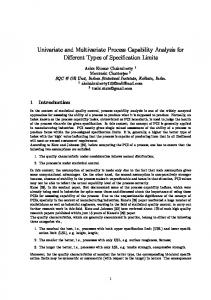
more powerful method of experimentation, as they are able to bring forth subtle yet significant differences among alternatives, even when none are evident in either corpora or through the forced-choice tasks (Featherston 2005). While corpus-derived results of alternative possible linguistic structures would tend to follow a Zipfian distribution (Zipf 1935, 1949), with the best-judged alternative also occurring with the relatively highest frequency, but the rest with very few if any occurrences at all, acceptability ratings of the same structures form a steadily declining linear continuum from the best-judged to the lowest-judged items, as is evident in Figure 1.1 below (Featherston 2005). Furthermore, according to Featherston, there would not appear to be any significant discontinuities among the range of alternative structures which would clearly divide them into grammatical and ungrammatical ones, the latter a view suggested by Kempen and Harbusch (2005) as well as Sorace and Keller (2005), with which I myself would be inclined to disagree. Nevertheless, from the overall perspective, acceptability ratings do not contradict corpus-based frequencies or selections in forced-choice tasks, since the best-judged alternatives are also relatively more frequent in corpora than the worse-judged alternatives. However, this relationship between the two types of evidence is asymmetrical because relative rareness does not directly imply acceptability; a rare item can be either fully acceptable or clearly unacceptable; nor does acceptability directly imply a high frequency (Arppe and Järvikivi 2007b). Nonetheless, as this earlier study was restricted to only two alternative synonyms and to only a few – though important – contextual features, my intention in this dissertation is to extend the scope of study to encompass both the number of alternative lexemes and the range of contextual features considered (to be revisited in Section 1.2).
Figure 1.1. The contrast between corpus (COSMAS9) frequency data and experimental judgement data on the same phenomenon (corresponding to Figure 1 in Featherston 2004: 52, and Figure 4 in Featherston 2005: 195).
9
The acronym COSMAS stands for Corpus Search, Management and Search system, which gives online access to the German language corpora of the Institut für Deutsche Sprache (IDS) in Mannheim, Germany, exceeding currently well over one billion words; URL: http://www.idsmannheim.de/cosmas2/.
6
Nevertheless, in comparison to the processing of corpora, experiments are considerably more time-consuming and laborious as well as subject to factors beyond the researcher’s personal control – after all, they require a substantial number of committed informants in a specified setting, perhaps also with special measurement instruments in order to produce scientifically valid results. Thus, using corpus-based analysis first to prune and select only a small set of the most relevant or otherwise interesting hypotheses for further testing with focused experimentation is well motivated on practical and economic grounds. Furthermore, despite the deficiencies of introspection as a primary source of evidence, a researcher can, and in fact has to use his linguistic intuition and introspection to interpret the results and to adjust the research hypotheses throughout the different stages and associated methods in the aforementioned research cycle (Cruse 1986: 10-11; Sampson 2001: 136-139; cf. “heuristic exploratory device” in Gries 2002: 27). As a final note, the concepts evidence, data and method are often used in an overlapping manner and may thus be difficult to clearly distinguish from one another. For instance, in the case of a corpus-based study, one could regard a corpus as the raw data, and evidence as simply various snippets selected from the corpus pertaining to the studied linguistic phenomenon, or in a varyingly more complex form the frequencies of various selected individual linguistic items and of their co-occurrences extracted from the corpus, and whatever analysis one can and might perform on this frequency information. As for what constitutes the method, one could, in the simplest case, consider making direct observations from a given corpus as the method; in the more complex analyses the observations would be based on a sequence of a variety of non-trivial tasks starting with the collection or selection of a corpus, its linguistic annotation, and the choice of appropriate statistical methods, and so on. So, in a sense, a corpus can play the role of raw data, of method and of evidence. 1.2
Synonymy and semantic similarity
The linguistic phenomenon studied in this dissertation is lexical synonymy, which I understand as semantic similarity of the nearest kind, as discussed by Miller and Charles (1991), that is, the closest end on the continuum of semantic distance between words. My general theoretical outlook is therefore linguistic empiricism in the tradition of Firth (1957), with meaning construed as contextual, in contrast to, for example, formal (de)compositionality (see, e.g., Cruse 1986: 22, Note 17; or Fellbaum 1998b: 92-94 for an overview of the relevant theories; or Zgusta 1971: 2747 for the classical lexicographical model employing the concepts designation/denotation, connotation, and range of application). Thus, I operationalize synonymy as the highest degree of mutual substitutability (i.e., interchangeability), without an essential change in the perceived meaning of the utterance, in as many as possible in a set of relevant contexts (Miller and Charles 1991; Miller 1998). Consequently, I do not see synonymy as dichotomous in nature, but rather as a continuous characteristic; nor do I see the associated comparison of meanings to concern truth values of logical propositions or conceptual schemata consisting of attribute sets. In these respects, the concept (and questionability of the existence) of absolute synonymy, that is, complete interchangeability in all possible contexts, is not a relevant issue here
7
Nevertheless, it is fair to say that I regard as synonymy what in some traditional approaches, with a logical foundation of meaning, has rather been called nearsynonymy (or plesionymy), which may contextually be characterized as “synonymy relative to a context” (Miller 1998: 24). However, like Edmonds and Hirst (2002: 107, Note 2), I see little point in expatiating on how to distinguish and differentiate synonymy (in general), near-synonymy, and absolute synonymy, especially since the last kind is considered very rare, if it exists at all. This general viewpoint is one which Edmonds and Hirst (2002: 117) ascribe to lexicographers, with whom I am inclined to align myself. A recent approach to synonymy which in my mind conceptually fleshes out the essence of this lexical similarity can be found in Cruse (2000: 156-160, see also 1986: 265-290), where synonymy is “based on empirical, contextual10 evidence”, and “synonyms are words 1) whose semantic similarities are more salient than their differences, 2) that do not primarily contrast with each other; and 3) whose permissible differences must in general be either minor, backgrounded, or both”. In the modeling of the lexical choice among semantically similar words, specifically near-synonyms, it has been suggested in computational theory that (at least) three levels of representation would be necessary to account for fine-grained meaning differences and the associated usage preferences, namely, 1) a conceptual-semantic level, 2) a subconceptual/stylistic-semantic level, and 3) a syntactic-semantic level, each corresponding to increasingly more detailed representations, that is, granularity, of (word) meaning (Edmonds and Hirst 2002: 117-124). In such a model of language production (i.e., generation), synonyms are grouped together as initially undifferentiated clusters, each associated with individual coarse-grained concepts at the topmost level (1), according to a (possibly logical) general ontology. The individual synonyms within each cluster all share the essential, core denotation of the associated concept, but they are differentiated in contrast to and in relation to each other at the intermediate subconceptual level (2), according to peripheral denotational, expressive and stylistic distinctions, which can in the extreme be cluster-specific and fuzzy, and thus difficult if not impossible to represent simply in terms of absolute general features or truth conditions. Consequently, a cluster of near-synonyms is nonetheless internally structured in a meaningful way, which can be explicable, even if in a complex or peculiarly unique manner. By way of example, the expressive distinction can convey a speaker’s favorable, neutral or pejorative attitude to some entity involved in a discourse situation, while the stylistic distinction may indicate generally intended tones of communication such as formality, force, concreteness, floridity, and familiarity. The last, syntactic-semantic level (3) in such a clustered model of lexical knowledge concerns the combinatorial preferences of individual words in forming written sentences and spoken utterances, for example, syntactic frames and collocational relationships. Though Edmonds and Hirst (2002: 139) do recognize that this level is in a complex interaction with the other two, they leave this relationship and the 10
One should note, however, that Cruse’s (1986: 8-10, 15-20) conception of contextual relations as the foundation of word meaning, and thus also synonymy, refers in terms of evidence rather to (the full set of) intuition-based judgments (possibly derived via experimentation) of the normality as well as the abnormality of a word in the totality of grammatically appropriate contexts, that is, including patterns of both disaffinity as well as affinity, and comparisons thereof, than the corpus-linguistic context of a word in samples of actually observed, natural language use (productive output in Cruse’s [1986: 8] terms).
8
specific internal workings of this level quite open. Working within this same general computational model, Inkpen and Hirst (2006) develop it further by also incorporating the syntactic-semantic level in the form of simple collocational preferences and dispreferences, though their notion of collocation is explicitly entirely based on statistical co-occurrence without any of the more analytical linguistic relationships (Inkpen and Hirst 2006: 12); they foresee that such contextual lexical associations could be linked with the subconceptual nuances which differentiate the synonyms within a cluster (Inkpen and Hirst 2006: 35). This fits neatly with the view presented by Atkins and Levin (1995: 96), representatives of more conventional linguistics and lexicography, that even slight differences in the conceptualization of the same realworld event or phenomenon, matched by different near-synonyms, are also reflected in their syntactic (i.e., contextual) behavior. In general, this aforementioned computational model also resembles psycholinguistically grounded models concerning the organization of the lexicon such as WordNet (Miller et al. 1990) to the extent that lexemes are primarily clustered as undifferentiated synonym sets (i.e., synsets) that are associated with distinct concepts (i.e., meanings), while semantic relationships are essentially conceived to apply between concepts, signified in practice by the synsets as a whole. However, the WordNet model fundamentally considers all lexemes belonging to such individual synsets as mutually semantically equivalent, effectively ignoring any synset-internal distinctions that might exist among them (Miller et al. 1990: 236, 239, 241; Miller 1995; Miller 1998: 23-24, Fellbaum 1998a: 9). Returning to the syntactic-semantic level, it has been shown in (mainly) lexicographically motivated corpus-based studies of actual lexical usage that semantically similar words differ significantly as to 1) the lexical context (e.g., English adjectives powerful vs. strong in Church et al. 1991), 2) the syntactic argument patterns (e.g., English verbs begin vs. start in Biber et al. 1998: 95-100), and 3) the semantic classification of some particular argument (e.g., the subjects/agents of English shake/quake verbs in Atkins and Levin 1995), as well as the rather style-associated 4) text types or registers (e.g., English adjectives big vs. large vs. great in Biber et al. 1998: 43-54), in which they are used. In addition to these studies that have focused on English, with its minimal morphology, it has also been shown for languages with extensive morphology, such as Finnish, that similar differentiation is evident as to 5) the inflectional forms and the associated morphosyntactic features in which synonyms are used (e.g., the Finnish adjectives tärkeä and keskeinen ‘important, central’ in Jantunen 2001, 2004; and the Finnish verbs miettiä and pohtia ‘think, ponder, reflect, consider’ in Arppe 2002, Arppe and Järvikivi 2007b; see also an introductory discussion concerning inflectional distinctions of synonyms in general in Swedish, Danish, and Norwegian Bokmål in Arppe et al. 2000). Recently, in their studies of Russian near-synonymous verbs denoting TRY as well as INTEND, Divjak (2006) and Divjak and Gries (2006) have shown that there is often more than one type of these factors simultaneously at play, and that it is therefore worthwhile to observe all categories together and in unison rather than separately one by one. Divjak and Gries (2006, forthcoming) dub such a comprehensive inventory of contextual features of a word as its Behavioral Profile, extending this notion to cover not only complementation patterns and syntactic roles as proposed by Hanks (1996),
9
who originally coined the concept, but any linguistic elements, whether phonological, morphological, syntactic, semantic, or other level of linguistic analysis, which can be observed within the immediate sentential context, adapting here the notion of the socalled ID tags presented by Atkins (1987).11 Furthermore, Divjak and Gries also present one possible way of operationalizing and compactly quantifying this concept for each word as one co-occurrence vector of within-feature relative frequencies. In my mind, one could alternatively refer to this concept as the Contextual Profile or Distributional Profile of a word, as its primary components are the occurrences and distributions of linguistically relevant items or characteristics (or their combinations) which can be explicitly observed in a word’s context in (a sample of) language usage. As noted earlier above, though Cruse’s (1986: 8-10, 15-20) concept of contextual relations is quite similar in both name and intended purpose in defining linguistic meaning, it fails to examine explicitly the individual elements in the context itself. All of these studies of synonymy have focused on which contextual factors differentiate words denoting a similar semantic content. In other words, which directly observable factors determine which word in a group of synonyms is selected in a particular context. This general development represents a shift away from more traditional armchair introspections about the connotations of and ranges of application for synonyms (e.g., Zgusta 1971), and it has been made possible by the accelerating development in the last decade or so of both corpus-linguistic resources, that is, corpora and tools to work them, such as linguistic parsers, and statistical software packages. Similar corpus-based work has also been conducted on the syntactic level concerning constructional alternations (referred alternatively to as synonymous structural variants in Biber et al. 1998: 76-83), often from starting points which would be considered to be anchored more within general linguistic theory. Constructional alternations do resemble lexical synonymy, for the essential associated meaning is understood to remain largely constant regardless of which of the alternative constructions is selected; however, they may differ with respect to a pragmatic aspect such as focus. Relevant studies concerning these phenomena have been conducted by Gries (2002) and Rosenbach (2003) with respect to the English possessive constructions (i.e., [NPPOSSESSED of NPPOSSESSOR] vs. [NP’sPOSSESSOR NPPOSSESSED]), Gries (2003a) concerning the English verb-particle placement, (i.e., [V P NPDIRECT_OBJECT] vs. [V NPDIRECT_OBJECT P]), and Gries (2003b) as well as Bresnan et al. (2007) concerning the English dative alternation, (i.e., [GIVE NPDIRECT_OBJECT PPINDIRECT_OBJECT] vs. [GIVE NPINDIRECT_OBJECT NPDIRECT_OBJECT]). The explanatory variables in these studies have been wide and varied, including phonological characteristics, morphological features and semantic classifications of relevant arguments, as well as discourse and information structure. With regard to Finnish, a good example of a syntactic alternation are the two comparative constructions, (i.e., [NPPARTITIVE ACOMPARATIVE] vs. [ACOMPARATIVE kuin NP], for example, Pekkaa parempi vs. parempi kuin Pekka ‘better than Pekka’, which is described by Hakulinen et al. (2004: 628-630 [§636-§637], and prescriptively scrutinized by Pulkkinen (1992 and references). These two alternative constructions last mentioned are cross-linguistically well known and studied, and are 11
Such an omnivorous attitude with respect to analysis levels and feature categories is an integral characteristic in machine learning approaches within the domain of computational linguistics.
10
considered to represent two distinct types in language-typological classifications (e.g., Stassen 1985, 2005). With the exception of Gries (2002, 2003a, 2003b), Rosenbach (2003), Bresnan et al. (2006), Divjak (2006), and Divjak and Gries (2006), the aforementioned studies have in practice been monocausal, focusing on only one linguistic category or even a singular feature within a category at a time. Though Jantunen (2001, 2004) does set out to cover a broad range of feature categories and notes that a linguistic trait may be evident at several different levels of context at the same time (2004: 150-151), he does not quantitatively evaluate their interactions. Bresnan et al. (2006) have suggested that such reductive theories would result from pervasive correlations in the available data. Indeed, Gries (2003a: 32-36) has criticized this traditional proclivity for monocausal explanations and has demonstrated convincingly that such individual univariate analyses are insufficient and even mutually contradictory. As a necessary remedy in order to attain scientific validity in explaining the observed linguistic phenomena, he has argued forcefully for a holistic approach using multifactorial setups covering a representative range of linguistic categories, leading to the exploitation of multivariate statistical methods. In such an approach, linguistic choices, whether synonyms or alternative constructions, are understood to be determined by a plurality of factors, in interaction with each other. More generally, this can in my mind be considered a non-modular approach to linguistic analysis. Nevertheless, the applicable multivariate methods need to build upon initial univariate and bivariate analyses. Furthermore, as has been pointed out by Divjak and Gries (2006), the majority of the above and other synonym studies appear to focus on word pairs, perhaps due to the methodological simplicity of such a setup; the same criticism of limited scope also applies to studies of constructional alternation, including Gries’ own study on English particle placement (2003a). However, it is clearly evident in lexicographical descriptions such as dictionaries that there are often more than just two members to a synonym group, and this is supported by experimental evidence (Divjak and Gries, forthcoming). Though full interchangeability within a synonym set may prima facie be rarer, one can very well assume the existence of contexts and circumstances in which any one of the lexemes could be mutually substituted without an essential change to the conveyed meaning. Consequently, the differences observed between some synonymous word pair might change or relatively diminish when studied overall in relation to the entire relevant synonym group. This clearly motivates a shift of focus in synonym studies from word pairs to sets of similar lexemes with more than two members, an argument which has already been expressed by Atkins and Levin (1995: 86). Finally, Bresnan (2007, see also 2006) has suggested that the selections of alternatives in a context, that is, lexical or structural outcomes for some combinations of variables, are generally speaking probabilistic, even though the individual choices in isolation are discrete (see also Bod et al. 2003). In other words, the workings of a linguistic system, represented by the range of variables according to a theory, and its resultant usage would not in practice be categorical, following from exception-less rules, but rather exhibit degrees of potential variation which becomes evident over longer
11
stretches of linguistic usage.12 These are manifested in the observed proportions of occurrence for one particular dichotomy of alternating structures, given a set of contextual features. It is these proportions which Bresnan (2007) et al. (2007) try to model and represent with logistic regression as estimated expected probabilities, producing the continuum of variation between the practically categorical extremes evident in Figure 1.2. Both Gries (2003b) and Bresnan (2007, et al. 2007) have shown that there is evidence for such probabilistic character both in natural language use in corpora as well as language judgements in experiments, and that these two sources of evidence are convergent. However, these studies, too, have concerned only dichotomous outcome alternatives.
Figure 1.2. Sample of estimated expected probabilities for the English dative alternation (reproduced from Bresnan 2006: 4, Figure 1, based on results from Bresnan et al. 2007).
12
From the perspective of understanding and explaining an empirical phenomenon, this means a shift from seeing causes as deterministic, “producing” an outcome by the “action of some universal and unfailing laws” to rather viewing causes as probablistic, which merely “increase the likelihood” of such an outcome (Hacking’s [1981: 113] interpretation of Fagot’s [1981] discussion concerning the causes of death within medicine).
12
1.3
Theoretical premises and assumptions in this study
The key theoretical concepts characterizing this dissertation are 1) contextuality, 2) synonymy, and 3) non-modularity (or constructionality). Firstly, I conceive meaning as fundamentally contextual in the spirit of Firth (1957), rather than as compositional or propositional. Thus, I assume a strong interconnection between (contextual) distributional and semantic similarity (cf. Divjak and Gries 2006: 27-28). However, as I am working with Finnish, a language having a relatively flexible word order, I operationalize context as grammatical rather than linear, that is, within a fixed window of words. Secondly, I take a naïve, lexicographical view with regard to synonymy (cf. Cruse 1986: 265; Edmonds and Hirst 2002: 116). That is, I take it as granted that the lexicon contains pairs or sets of words which are mutually interchangeable without an essential change in their core conveyed meaning. Nevertheless, I suspect that this mutual interchangeability is not, and need not, be categorical. In terms of the contextual view, synonymy consequently means for me interchangeability in many/most contexts, but not necessarily all. Thirdly, I am a nonmodularist with respect to linguistic analysis. In my view, regularities in cooccurrence and structure can be observed along an ungraded continuum with increasingly more abstract levels, from fixed collocations concerning words and morphemes up to conventional syntactic structures composed of general parts of speech or semantic classes of words. Nevertheless, we will often find it practical to segment linguistic analysis into several conventional levels such as morphology, syntax and semantics, but this does not to my mind require or lead to treating these levels as fully independent of, autonomous of, and detached from each other. This attitude towards linguistic analysis can be viewed as constructional, following Construction Grammar (e.g., Croft 2001); however, I will not adhere exclusively to any single linguistic theory in this dissertation. 1.4
The goals of this study and its structure
This dissertation is first and foremost a methodological study. My specific goal is to extend the study of one type of linguistic alternation, that is, synonyms and their choice, from dichotomous to polytomous settings, involving the lexical choice among more than two alternatives. Likewise, my purpose is also to move from simplistic, univariate explanatory models of lexical choice to more complex but powerful multivariate ones, explaining the phenomenon in question with a broad, representative range of linguistic and extralinguistic variables. Therefore, as a follow-up to Arppe and Järvikivi (2007b), the other members of the Finnish THINK synonym group with frequencies within the same (relatively high) magnitude as the original pair, have been selected for scrutiny in this study, resulting in the lexeme set ajatella, miettiä, pohtia and harkita. Furthermore, instead of considering only the morphological structure or one specific argument of the studied verbs, as was the case in the former study, the range of contextual features included in the analysis in this dissertation will be extended to cover the entire syntactic argument structure of the studied verbs and the semantic subclassifications of the individual argument types, including extralinguistic features such as text type and register. In terms of linguistic description, my purpose is to demonstrate how lexemes in a synonym group are used differently on the basis of their context, and to lay out the
13
individual features which determine these differences as well as assess their relative importance and weights. Ultimately, this should result in better descriptions of the lexemes I have chosen to study, and by way of replication, the overall improvement of broad-coverage lexicographical descriptions such as dictionaries. As for the development of linguistic research methodology, in this dissertation I intend to explain in detail why I have selected particular statistical methods and how these are in practice applied to corpus data, and, using examples, demonstrate how the results can be interpreted, thus also showing what the selected statistical methods have to offer from the linguistic perspective. This will be an exploratory study, with no specific hypotheses to prove or disprove other than the general assumption of the existence of differences in contextual preferences and dispreferences among the studied THINK lexemes, whatever the actual features involved may turn out to be. Consequently, the number of different individual features and feature categories covered in this study will be substantial. On the general level, this setup of including a wide range of different features as well as a broader set of synonyms than a simple pair largely resembles that of Divjak and Gries (2006). However, my focus is rather on discovering features distinguishing the members of a synonym group from each other than on the internal grouping of a synonym set that these features also reveal. Furthermore, I will take the groupings of synonyms mostly as they are given in current, authoritative Finnish dictionaries, and I will not delve deeper into what corpus-based contextual evidence could indicate in this respect. Thus, of the three main challenges that Divjak and Gries (2006: 24-27) present for the study of synonyms, namely, 1) the lexicon-general delineation of words into synonym groups, 2) the internal structuring of these groups, and 3) the description of features which differentiate the individual synonyms from each other, my dissertation will focus on the third and last task. As Divjak and Gries (2006: 2324) note, synonymy has received within Western linguistics far less attention in linguistic research than other lexical relationships such as polysemy. Though this “neglect” has to some extent been remedied by a string of recent studies both in Finland (e.g., Jantunen 2001, 2004; Arppe 2002; Arppe and Järvikivi 2007b; Vanhatalo 2003, 2005; Päiviö 2007) and abroad (e.g., Edmonds and Hirst 2002; Inkpen and Hirst 2006; Divjak and Gries 2006), the topic is neither far from exhausted nor conclusively resolved. Thus, one general objective of this study is to continue this trend as a worthwhile linguistic research topic and contribute to our understanding of synonymy as a linguistic phenomenon. The long-term purpose of my research is to increase our understanding of what the relationship is between naturally produced language, that is, corpora, and the posited underlying language system that governs such usage. This concerns both 1) the use and choice among lexical and structural alternatives in language and 2) the underlying explanatory factors, following some theory representing language as a comprehensive system. A subsequent subservient methodological objective is how this can be modeled using various statistical methods with different levels of complexity, ranging from the univariate to the multivariate levels. A question which may at first glance appear secondary but which will turn out to be of general theoretical import is to what extent we can describe the observed variation in terms of the selected analytical features that conventional linguistic theory incorporates and works upon.
14
The structure of this study is as follows. In Section 2, I will begin by presenting the various linguistic aspects of this study, including the selection of the studied synonyms, the general principles of the various levels of linguistic analysis which are to be applied to the research corpus, and a description of the compilation as well as the characteristics of the selected research corpus. The individual levels of analysis and the associated specific features are fully presented in Appendix C. Furthermore, I will tease out what current lexicographical descriptions of the selected synonyms reveal about their usage, whether explicitly or (mostly) implicitly, in terms of the same features of linguistic analysis applied in this study, in order to provide a benchmark against which to compare the corpus-based results to follow later on. In Section 3, I will move on to lay down the battery of statistical methods to be used in this dissertation, starting off with several univariate methods, extending some of these to bivariate analysis, and finishing with multivariate methods, concentrating on polytomous logistic regression. Among the univariate methods, I will first address the assessment of the overall homogeneity/heterogeneity of a distribution and various follow-up tests, and then a more comprehensive exposition of various measures of association for nominal (non-ordered categorical) variables. The bivariate analysis methods will in fact be applications of the very same measures of association presented among the univariate methods. In addition, I discuss extending the method presented by Gries (2003a) from dichotomous to polytomous settings. Regarding the multivariate analysis methods, I will conclude by also presenting various ways of assessing the robustness and generalizability of the forthcoming results, with a major focus on bootstrapping procedures of several kinds. Throughout this Section, I will use only a limited set of linguistic analysis features, typically anchored in previous research if such exists, to take a detailed walk through the successive stages of the actual calculations, not to mention the various ways in which the thus retrieved results can be abstracted and interpreted from a linguistic perspective. In Section 4, I will begin to show the results of applying these various statistical methods using the selected linguistic analysis features, again proceeding from univariate through bivariate to multivariate results. Here, I will present only the very last, abstracted end of the underlying statistical calculations, which will often be the result of several layers of simplification and interpretation. For those interested in specific analyses by each level and feature categories or the actual underlying figures, these can be found in the Appendices, while the details of their calculation have been exemplified earlier in Section 3. Among the univariate results presented in Subsection 4.1, I will begin with general observations of the feature-specific values of the selected measures of association, concluding with an attempt at post hoc generalizations presented in Subsection 4.1.2 and, finally, a comparison of the univariate results with existing lexicographical descriptions in Subsection 4.1.3. The bivariate results discussed in Subsection 4.2 will most importantly prepare the ground for the considerable pruning down of the feature variables selected for the multivariate analyses covered in Section 5. Here, I will compare the performance of different techniques for implementing polytomous logistic regression for the full selected variable set as well as the explanatory power of different subsets of the selected variables representing varying degrees of analytical depth or intricacy. This will be followed by a full exposition of the feature-wise weights, that is, the estimated odds, for the finally selected feature set, and then an assessment of the robustness of the results with several techniques. Next, I will discuss at length the probability
15
estimates that polytomous logistic regression conveniently produces for each lexeme with respect to any combination of features incorporated in the developed model. This general Section 5 discussing the results will end in Subsection 5.6 with a suggestion for the new description of the studied synonyms building specifically upon the multivariate results, to be compared with the current ones analyzed earlier in Subsection 2.3. For the most part, I will in Sections 4 and 5 link and discuss the specific observations and conclusions reached in this study with regard to previous research at those points when they are first encountered and presented, leaving only the most general conclusions to Section 6. In this next-to-last section, I will also sketch hypotheses for later experimentation, not to mention other ensuing areas for further research, many of which I have had to exclude from this dissertation due to limitations of space. Finally, a short overall conclusion highlighting the main results of this dissertation will be presented in Section 7. For a linguistically minded reader, either Section 4.1.2 presenting the post hoc general characterizations of the studied THINK lexemes, or Section 5.6 laying out the new lexicographical description scheme resulting from the multivariate analysis results, with pohtia as an example, might be the best starting points for getting a concise overview of what this dissertation is about in lexicographical terms. In addition to the main text, the Appendices contain a wealth of information that I believe will be of genuine value and interest, but which is not integral to the central objectives of this dissertation. Moreover, a comprehensive collection of the data used in this study, the research corpora and their linguistic analyses, the scripts with which they have been processed and the tailored functions with which the statistical analyses have been undertaken in the R statistical computing environment, as well as the complete results, can all be found in the amph microcorpus under the auspices of CSC Scientific Computing, .
16
2
Data and its linguistic analysis
2.1
Selection of the studied synonyms
2.1.1
Background in prior studies
The set of four synonymous THINK lexemes scrutinized in this study, ajatella, miettiä, pohtia, and harkita, were first and foremost selected because I had in earlier studies on my own and in co-operation with others focused extensively on one pairing among them, namely, miettiä vs. pohtia, which I had considered semantically the closest ones of the group (Arppe 2002; Arppe and Järvikivi 2002; Arppe and Järvikivi 2007b). Although pairwise comparisons of synonyms are by far the most common in linguistics, perhaps in part because it is methodologically the easiest setting to pursue, synonymy as a phenomenon is by no means restricted to word pairs either conceptually or in practice, nor should its study be limited to such pairs, as Divjak and Gries (2006) argue and demonstrate, nor. For instance, we can find in dictionaries and thesauri often more than one synonym provided for many of the lexical entries. From my own experience, however, I must concede that in the case of most synonym sets, one can without much difficulty come up with contexts or connotations that clearly distinguish individual synonyms from the rest, often leaving one with only one pair (or pairs) which at least superficially are not immediately distinguishable from each other on the basis of one’s professional (and native speaker’s) linguistic intuition. The original selection of the miettiä-pohtia synonym pair and the entire synonym set of THINK verbs to which they belong was based on a rigorous process with the purpose of identifying lexemes for which their syntactic and semantic valency profiles as well as the “contamination” effect from their possible polysemous senses, and even extralinguistic factors such as their relative frequencies, should be as similar as possible (due to the frequency effect13 in linguistic processing, for which an overview is presented in Ellis 2002). The ultimate goal was thus to ensure a priori a degree of interchangeability as high as possible in the observable contexts, as a proxy for the nearest possible synonymy. Of course, one could have used a quantitative method such as the sub-test presented by Church et al. (1994) or its modification using exact statistics as suggested by Gries (2003c) to assess such factors empirically. However, because the present study, as well as my earlier ones, specifically use a corpus to uncover usage-based similarities and differences, I regarded other sources, independent of the chosen type of direct empirical evidence, as more appropriate. These sources are the Suomen kielen perussanakirja in its various editions and forms (Haarala et al. 1994-1997, Haarala et al. 1997), that is, ‘The Standard Dictionary of Finnish’ hereafter denoted by the acronym PS, and the comprehensive descriptions of Finnish verbs by Pajunen (1982, 1988, 2001), which are all corpus-based, though each uses a different, yet in some cases overlapping, selection of source material. In addition, the predecessor to PS, Nykysuomen sanakirja (Sadeniemi et al. [1951-1961] 1976), ‘Dictionary of Modern Finnish’ hereinafter denoted by the acronym NS, is also 13
Simply put, the frequency effect in the case of lexis means that the “recognition and processing of words is a function of their frequency of occurrence in the language” (Ellis 2002: 152); however, the underlying factors behind this empirical observation have been shown to be more complex than the simple definition would lead to believe, see, for example, Balota and Chumbley (1985), Schreuder and Baayen (1997), and Dahan et al. (2001).
17
consulted specifically in Section 2.3.2, which presents the extent to which the usage of studied lexemes has been described until now. The NS is a very comprehensive and extensive lexicographical work, which, exceeding 200,000 lexical entries, is almost twice the size of PS. However, it has essentially not been updated since it was compiled in 1929-1961 and is thus based on Finnish in the form it was used (and conceived to be) in the first half of the twentieth century. For this reason, I have primarily relied on the more up-to-date PS, as its contents have been during its existence since 1994 and thereafter under an on-going revision process by Kotimaisten kielten tutkimuskeskus (KOTUS), the ‘Research Institute of the Domestic Languages in Finland’ , and even more so as PS in fact incorporates much of NS’s central content.14 In order to rule out pairs or sets of lexemes with potentially marked members resulting from relative infrequency, synonym candidates in the preceding studies were first ranked both by pairs and by entire sets according to the geometric averages of their relative frequencies (in the case of synonym sets considering only the values of their non-null members), based on a million-word corpus sample of Finnish newspaper text (a portion from Keskisuomalainen 1994),15 so that pairs or sets with high but at the same time also relatively similar frequencies came first. The synonym sets were extracted from the lexical database underlying the FINTHES inflecting thesaurus software module developed at Lingsoft.16 Using my own linguistic intuition as a native speaker of Finnish, I then scrutinized this ranking list from the top down in order to pick out promising candidates. In turn, these were evaluated in depth with respect to the similarity of their semantic and syntactic valency structures using both the specific descriptions by Pajunen (1982: 169, 180-182), when existent, and the definitions and usage examples from the lexical entries in PS (Haarala et al. 1997). Regarding the first reference work, in its earlier form it covered explicitly only the most frequent or representative lexeme (or two) for each semantic field corresponding to a synonym group, in comparison to the more comprehensive coverage in its later, substantially revised extension (Pajunen 2001). This current version, however, had not yet appeared at the time of the initial research and it is still more exemplifying 14
Not to make things any less complicated, the latest versions of PS have in fact been marketed and distributed since 2004 under the name of Kielitoimiston sanakirja ‘The Dictionary of the Finnish Language Office’ (at KOTUS), denoted by the acronym KS. In terms of both its content and structure, KS is essentially an updated version of PS. 15 N.B. This subsample was part of the corpus used in my earlier studies (Arppe 2002; Arppe and Järvikivi 2007b), but not the part of the corpus material used in this study. 16 This Finnish synonym database was originally compiled by Katri Olkinuora and Mari Siiroinen for Lingsoft at the behest of professor Kimmo Koskenniemi between 1989-1991 (see Arppe 2005b). This database has 7439 entries overall and approximately 29854 words (when not distinguishing multi-word synonyms as distinct units). These figures are certainly less than what could be extracted from the PS (Haarala et al. 1997) by treating the single-word definitions as synonyms, amounting to synonym candidates for 35067 out of the altogether 102740 entries, containing 506212 words, but compared to the PS the FINTHES database contains explicitly only synonyms, and its electronic version was/is considerably simpler to process as it has been supplemented with word-class data lacking from PS. Unfortunately, FINTHES has not been publicly documented. Another synonym dictionary of Finnish that must be mentioned is the one appended to NS, Nykysuomen sanakirjan synonyymisanakirja (Jäppinen 1989), which contains some 18000 lexical entries. However, it appears that at least in the case of the studied THINK lexemes the synonym sets in this work correspond quite closely to the singleword definitions in PS, which is not that surprising as both works build upon NS. Therefore, I have relied on PS, even more so, as it was at my disposal in electronic form.
18
than exhaustive in nature.17 Nevertheless, even though the terminology and structure of Pajunen’s general ontology and description has changed somewhat over time (cf. the tables/diagrams in Pajunen 1982: 336 in comparison to Pajunen 2001: 51-57, noted sketchily in Arppe 2006b), the conclusions as to the very close similarity of the argument structure of the selected THINK lexemes remain the same, though the picture has become more detailed. In contrast, the second reference work (PS) has remained quite stable over the last decade, even more so as it is directed to a larger, non-professional audience. In its case, semantic similarity was assessed in terms of the extent to which the candidate synonyms shared the same words as definitions and the degree to which they could be judged substitutable with each other in the typically several usage examples given in the dictionary entries. In the end, this process had originally yielded several promising synonym groups, such as the THINK18 verbs ajatella, miettiä, pohtia, harkita, and tuumia/tuumata ‘think, ponder, consider, reflect’ as well as the UNDERSTAND verbs ymmärtää, käsittää, tajuta, and oivaltaa ‘understand, grasp, comprehend’.19 Out of these, the pair miettiä-pohtia ‘think, ponder’ had been chosen (see Appendix A for an evaluation of the mutual interchangeability of these and the other THINK verbs in the example sentences given in the respective entries in PS), with their semantic similarity further validated by me through a manual assessment of the mutual interchangeability in each of the individual 855 sentences containing an instance of this verb pair in the originally used corpus (Keskisuomalainen 1994). The requirement satisfied by the miettiä-pohtia pair was thus that of strong entailment, meaning that interchangeability applies for all (or practically all) cases. In this original selection process, it appeared to me that this strict criterion for the degree of substitutability will probably yield in larger numbers only pairs of synonyms, which are also common/frequent enough to be representative of general linguistic usage, and consequently the requirement would have to be relaxed somewhat in the case of synonym sets with more than two members. For instance, WordNet is based on a weaker notion of entailment, where interchangeability in at least some context(s) suffices for synonymy (Fellbaum 1998b: 77; Alonge et al. 1998: 21).
17
For instance, only ajatella and miettiä are explicitly mentioned in Pajunen (1982), whereas ajatella, tuumia, harkita, miettiä, and järkeillä are noted at various points in Pajunen (2001: 63, Table 8, 314, 317) (but still not pohtia). 18 Interestingly, THINK is one of the proposed semantic primes concerning mental predicates in natural semantic metalanguage, that is., NSM, (e.g., Goddard 2002, Table 1.2), a theory originally proposed by Wierzbicka (1996), although I was not aware of this at the time of the original selection process. 19 In the original frequency ranking using FINTHES and selecting only verb sets, the THINK verbs were to be found at rankings 51, 143, and 500 (with miettiä and pohtia together at the last mentioned ranking); the UNDERSTAND verbs were to be found at ranking 217.
19
Figure 2.1. The semantic classification hierarchy of MENTAL verbs according to Pajunen (2001)
In order to establish and demarcate the extended group of synonymous THINK lexemes to be scrutinized in this dissertation, I will try to improve the above process by repeating it with a more comprehensive dictionary and a substantially larger corpus. I will first conduct a variant of the sub-test by using dictionary content from PS (Haarala et al. 1997), with the purpose of studying the overlap of word-definitions for lexemes belonging to the more general semantic grouping of COGNITION verbs, one step up from the THINK synonym group in Pajunen’s (2001) hierarchy (see Figure 2.1). This will produce pair-by-pair ratings of similarity and dissimilarity for each lexeme against each other, for all those which are included in the analysis. Then, I will assess the resultant candidate synonym groupings with respect to the similarities/differences in the magnitudes of their relative frequencies, calculated on the basis of the largest corpus collection currently available for Finnish, namely, the Finnish Text Collection (FTC 2001). 2.1.2
Screening out the interrelationships of COGNITION lexemes by their dictionary definitions
I will begin with Pajunen’s (2001: 313-314) treatment of COGNITION verbs, for which she distinguishes six different subclassifications. These consist of verbs of ANTICIPATION, e.g., aanailla, ounastella ‘anticipate/foresee’, vaistota ‘sense’, uumoilla ‘guess [in a roundabout, unsure way]’; verbs of BELIEF and ASPIRATION, e.g., epäillä ‘suspect/doubt’, haaveilla ‘dream’, kuvitella ‘imagine’, luulla ‘think/believe’, mieliä ‘aspire/desire to’, toivoa ‘wish/hope’, and uskoa ‘believe’; verbs of THOUGHT PROCESS and STATE OF KNOWLEDGE, e.g., ajatella ‘think’, harkita ‘consider’, järkeillä ‘reason’, käsittää ‘grasp/understand’, miettiä ‘think/ponder’, muistaa ‘remember’, tietää ‘know’, tuumia ‘think/reflect/muse’, ymmärtää ‘comprehend’; EVALUATIVE verbs, e.g., arvioida ‘evaluate/judge’, huonoksua ‘consider bad’, väheksyä ‘belittle’, paheksua ‘consider improper’, paljoksua ‘consider as [too] much’, puntaroida
20
‘weigh’, and verrata ‘compare’; verbs of INTENTION, e.g., aikoa, meinata ‘intend’, suunnitella ‘plan’, tarkoittaa ‘mean/intend for’; and verbs of ABILITY/CAPABILITY, e.g., jaksaa ‘have the strength to’, kehdata ‘dare/have the nerve to’, kyetä ‘can/have the capability to’, onnistua ‘succeed in’, osata ‘know how to’, and pystyä ‘can/be able to’. As the last subgroup is typically considered part of the Finnish modal verb system (see Kangasniemi 1992), I will exclude them from further scrutiny here. Using these 31 (exemplified) COGNITION verbs explicitly mentioned by Pajunen (2001: 313-314) as a starting point, I first selected from PS all the dictionary entries in which any one of Pajunen’s examples was listed either as an entry lexeme or among the single-word definitions. This yielded 114 entries with 465 single-lexeme definitions, which consisted of 96 unique entries and altogether 168 unique lexemes, with which the same selection process was repeated once more, this time yielding 566 entries with 1498 single-lexeme definitions, representing 422 unique entry lexemes associated with 630 unique lexemes. If an entry lexeme had several explicitly indicated (i.e., numbered) distinct senses, that particular lexeme is listed repeatedly, each time together with those word-definitions that are associated with the sense in question. As a consequence, some word-definitions may also be counted in more than once for some particular entry lexemes, in such a case indicative of a shared range of senses with the recurrent word-definitions. An example of the thus extracted word definitions for our old friends miettiä and pohtia is presented in Table 2.1. We can immediately see that miettiä has slightly more individual definition words than pohtia (9 vs. 7); furthermore, as many as 6 are common for both, in addition to both named as a definition of the other. The full list of the selected COGNITION lexemes is given in Table B.1 in Appendix B, together with frequency information to be discussed below. Table 2.1. Single-word definitions in PS for miettiä and pohtia; common lexemes in boldface (no lexemes with repeated occurrences among the word-definitions). Entry Single-word definitions miettiä punnita, harkita, ajatella, järkeillä, tuumia, mietiskellä, pohtia, suunnitella, aprikoida pohtia punnita, harkita, ajatella, järkeillä, tuumia, miettiä, aprikoida
The purpose was to canvas in this manner any lexemes which in at least one of their senses could be used to denote a COGNITION state, process or activity. Therefore, no lexemes were excluded from the final set even though they obviously primarily denoted some other semantic field. Among these cases were, for instance, nähdä ‘see’ in the sense of UNDERSTAND, as if mentally “seeing”, haistaa ‘smell/sniff’, used figuratively as ‘get a whiff of something’, or hautoa, literally ‘incubate’ but also ‘hatch a plan (by oneself/in secret), foment, brood (long/alone)’. Furthermore, considering the entire COGNITION group instead of only the THOUGHT PROCESS subclass allowed also for assessing the degree of polysemy among the constituent lexemes, as some can clearly be considered to belong to more than one of the subclassifications, for instance ajatella as denoting both a THOUGHT PROCESS and INTENTION. My hypothesis was that quantitative analysis would link close in similarity those lexemes for which all the senses, or at least the primary ones, are associated primarily with COGNITION and any of its subclasses, while lexemes with multiple senses of which only one, possibly secondarily, concerns COGNITION, or which belong to more than one of its subclasses, would be relegated to the fringes.
21
With these word lists we can now quantify for each and every pairing of the selected COGNITION entry lexemes the extent of overlap among their definitions, which corresponds in principle to the sub-test (Church et al. 1994), but with single-word definitions used instead of significant collocates. The more word-definitions a lexeme has in common with another, the more intersubstitutable they can be considered, though this may be due to not only synonymy but also other types of lexical relationships between the two lexemes such as hyponymy or even antonymy, as Church et al. (1994) point out. However, using word-definitions instead of collocates, which Church et al. 1994 focused on, should specifically target synonymous lexemes. The resulting lists of lexemes similar in this respect with miettiä and pohtia are presented in Table 2.2. This time, we can see that miettiä has common word-definitions with 25 of all the other COGNITION lexemes, whereas the corresponding figure for pohtia is slightly less at 23. Furthermore, in the case of both entries there are several other lexemes with which they share quite many word-definitions, indicating a closer relationship. Most notably, both share the most number of word-definitions with ajatella, tuumia and aprikoida in addition to each other. In fact, both miettiä and pohtia have 19 lexemes (plus each other), with which they both share at least one word-definition, suggesting that the two lexemes would appear to be quite substitutable with one another. This overlap fits Pajunen’s (62-63) assessment well that the classificatory structure of MENTAL verbs in general consists of lexical sets in which the members are in loose cohyponymic relationships with each other. However, a substantial number of noncommon lexical entries are also evident, which indicates that the lexemes are not exact synonyms in relation to each other. Table 2.2. Overlap among the single-word definitions of miettiä and pohtia with all the selected COGNITION lexemes; common lexemes in boldface. Lexeme (number Lexemes with overlap in definitions of lexemes with (number of overlapping items) overlap) miettiä (38) ajatella (7), pohtia (6), tuumia (5), aprikoida (5), järkeillä (4), filosofoida (4), harkita (3), hautoa (3), funtsata (3), punnita (2), aikoa (2), tutkailla (2), tarkoittaa (2), tutkistella (2), spekuloida (2), meinata (2), meditoida (1), laatia (1), hankkia (1), tarkastella (1), ohjelmoida (1), katsoa (1), muistaa (1), pähkäillä (1), punoa (1), konstruoida (1), tuumailla (1), mitata (1), sommitella (1), arvella (1), mietiskellä (1), laskea (1), mitoittaa (1), tykätä (1), pohdiskella (1), keskustella (1), käsitellä (1), luonnostella (1) pohtia (23) ajatella (6), miettiä (6), tuumia (4), aprikoida (4), funtsata (3), punnita (2), harkita (2), muistaa (2), järkeillä (2), filosofoida (2), hautoa (2), aikoa (1), katsoa (1), tuumailla (1), kelata (1), mitata (1), arvella (1), tarkoittaa (1), mietiskellä (1), laskea (1), spekuloida (1), tykätä (1), meinata (1)
In order to construct larger synonym sets, we could compare manually the overlap of the word-definitions for three, four or even more lexical entries. This is a feasible approach if we have a prior idea regarding which of the lexemes we want to consider (and thus also the size of the potential synonym set). In the case of the THINK lexemes, on the basis of my native speaker competence of Finnish and the two sets of overlapping lexemes presented in Table 2.2, I would be inclined to select as a
22
synonym set ajatella, pohtia, tuumia, aprikoida, järkeillä, harkita, hautoa, punnita, and tuumailla, with possibly also filosofoida and funtsata, the latter two lexemes being somewhat marked as sarcastic and slang terms, respectively. The worddefinition overlaps for all of these entry lexemes, similar in form to those presented in Table 2.2, are presented in Table B.2 in Appendix B. In fact, this hypothesized synonym list overlaps with the synonym list anchored around miettiä (and shared by ajatella, pohtia, harkita and tuumia) in Jäppinen (1989), consisting, namely, of, ajatella, miettiä, mietiskellä, pohtia, pohdiskella, harkita, tuumia, aprikoida, järkeillä, puntaroida, punnita, tuumata/tuumailla, hautoa, filosofoida, meditoida, spekuloida, and funtsata/funtsia (where overlapping lexemes are in boldface). However, without such a hypothesis a blind exploratory comparison of all the possible permutations of trios and larger sets quickly becomes exceedingly large with even a relatively small number of lexical entries under overall consideration, with the number of permuted sets amounting to npermutations = nentries!–(nentries–nset_size)!, and there would be no simple way to establish the proper size of synonym sets. 2.1.3
Clustering the COGNITION lexemes with statistical means
Under such circumstances, we may resort to a multivariate statistical method such as hierarchical agglomerative cluster analysis (HAC) (e.g., Kaufman and Rousseeuw 1990, see also Baayen 2007: 148-160), similar to what Divjak and Gries (2006) demonstrate, but by using either the single word definitions as such or the extent of their overlap as the classifying variables instead of contextual features derived from a corpus. A specific technique belonging to family of cluster analysis methods, HAC starts by considering all the items as singular clusters, which it then iteratively combines into larger clusters on the basis of maximizing intra-cluster similarity and minimizing inter-cluster similarity at each stage, ending up with a hierarchically nested tree structure. This data structure is typically represented as a so-called dendrogram, a sort of tree structure, which allows us to scrutinize visually the relationships of the individual items and then determine an appropriate set of clusters. We can thus use this technique to cluster the entire set of selected COGNITION lexemes either according to 1) the single-word definitions as such and 2) the extent of overlap with respect to these single-word definitions, the complete results of which are presented in Figures B.1 and B.2 in Appendix B.20 Interestingly, one can clearly discern in the overall dendrograms a distinct subcluster for THINK lexemes as well as another one for UNDERSTAND lexemes, with both of these sets being adjacent, and thus similar as groups, to each other. However, the overall hierarchy appears quite flat, and within the two subgroups “bushy”, which is in accordance with Pajunen (2001: 62-63, 313, see also Note 8 on page 434).
20
As Divjak and Gries (2006: 37) note, there are several ways of calculating the similarity of the items and for determining the criteria for the amalgamation of the clusters, the selection of which significantly influences the resulting cluster structure. However, there are no deterministic, universally applicable rules for selecting these methods, which would guarantee an optimal solution. As Divjak and Gries have done, I have selected the methods that appear to produce the most useful results, these being the default Euclidean distance as a measure of (dis)similarity (in contrast to the Canberra method chosen by Divjak and Gries) and Ward’s rule as the strategy for combining clusters (as did Divjak and Gries).
23
The two subclusters of THINK lexemes constructed with the two types of variables are presented in Figures 2.2 and 2.3, respectively. In general, we can see that the THINK subcluster based on the overlap corresponds exactly to the semantically hypothesized synonym set, whereas the subcluster based on the individual single-word definitions includes some additional lexemes. As these appear all in the overlap lists for miettiä and pohtia, they can in some sense be used to denote the THINK concept. However, they are in my judgement either rarer and semantically quite specific lexemes, namely, filosofoida ‘philosophize, think philosophically/excessively theoretically (literally: to make philosophy out of something)’, pohdiskella ‘contemplate, ponder (aloud, now and then, not too seriously)’ or pähkäillä ‘think over (and over)’, or their primary sense is divergent from THINK “proper”, namely, spekuloida ‘speculate (out loud)’, meditoida ‘meditate’, tutkailla and tutkiskella ‘examine (study in one’s mind)’, muistaa ‘remember’, meinata and tarkoittaa ‘mean (intend to say)’. This judgement is also supported by their low degree of overlap. Interestingly, ajatella is clearly separated from all the rest in the overlap-based diagram (Figure 2.3), which could be explained by its role as the most frequent and prototypical of the group, as well as by its broad range of senses (see Section 2.3.2 below).
Figure 2.2. Subcluster of THINK lexemes on the basis of all the single-word definitions of the COGNITION lexemes.
24
Figure 2.3. Subcluster of THINK lexemes on the basis of their overlap with respect to the single-word definitions.
2.1.4
Extracting frequencies for THINK lexemes
Next, I calculated the frequency rankings for all the verb lexemes in PS (Haarala et al. 1997) using the (base-form) lexeme frequency counts from the Finnish Text Collection (FTC 2001), the largest uniformly processed collection of Finnish to date. This corpus combines Finnish newspaper, magazine and literature texts from the 1990s, and amounts to some 180 million running text tokens. The corpus has been morpho-syntactically analyzed and disambiguated in its entirety using the Textmorfo parser (Jäppinen et al. 1983, Jäppinen and Ylilammi 1986, Valkonen et al. 1987) developed at Kielikone ; one should remember, however, that the results have not been manually verified and, what is more, no distinctions are obviously made between polysemous senses. In this corpus, a total of 25.4 million instances (roughly 14% of the running word tokens) were analyzed as verbs, representing 20930 distinct base-form lexemes. Of these, roughly over a half (12983) have at least two or more occurrences. This time, I used the natural logarithm of the relative frequency as an indicator for the magnitude of lexeme frequency (instead of the raw absolute or relative values as such), and the arithmetic average of these logarithm values as an indicator for the joint magnitude of the frequencies of a lexeme group as constituted by an entry and its single worddefinitions (with only non-zero values included in the calculation). The frequencies and the individual and joint rankings of the 566 selected COGNITION entry lexemes and their associated single-word definitions are presented in full in Table B.1 in Appendix B. We can now assess the relative frequencies of the subcluster of THINK lexemes identified above on the basis of the overlap in the single-word definitions (see Table 2.3). For the sake of comparison, Table 2.3 also contains the rankings from the Frequency Dictionary of Finnish (denoted FDF hereinafter) by Paunonen et al. (1979), which are also corpus-based figures.21 Interestingly, there is variation among 21
This Frequency Dictionary of Finnish is based on a corpus containing Finnish fictional texts, radio discussions, newspaper and magazine texts, and non-fiction reference works from the 1960s,
25
the individual rankings calculated here and those from the earlier source, though the orderings are overall quite similar: frequent lexemes in FTC are also frequent lexemes in the FDF, while infrequent lexemes here are again infrequent in FDF, if ranked at all. As can be seen, the magnitudes as represented by the natural logarithms of the relative frequencies are very close for the three most frequent lexemes, namely, pohtia, ajatella and miettiä, followed by harkita and tuumia, each alone on the next steps down on the magnitude ladder, before the rest of the more infrequent lexemes in the set. Indeed, visual inspection of Figure 2.4 also indicates that the observed frequencies of the scrutinized lexemes do not exactly conform to an ideal Zipfian distribution (see Appendix K), which is also supported by a goodness-of-fit test (with P=0).22 On the basis of these results, I decided to select for further study in this dissertation the four most frequent lexemes in the THINK group, namely, ajatella, miettiä, pohtia, and harkita. In addition to clearly trailing harkita, the fifth-ranked tuumia has in comparison to the three most frequent lexemes only about one-tenth of occurrences. Furthermore, we will observe that in the final research corpus, described below in Section 2.4.2, tuumia has only 47 occurrences, which will be too low for the statistical analyses; the other THINK lexemes ranked as infrequent here have even fewer occurrences in the research corpus. Interestingly, it is exactly the selected set of four THINK lexemes which are given as the single-word definitions for the modern colloquial funtsata/funtsia. Moreover, we will later find out in Section 2.3.3 that three out of the four finally selected THINK lexemes, namely, ajatella, pohtia and harkita, have etymological origins in concrete activities of rural life particular to Finland, with the sole exception of miettiä as a loan word. It will turn out that some vestiges of these concrete meanings can be interpreted to persist among the contextual preferences of the now abstract usages of these particular THINK lexemes.
amounting to slightly over 408 thousand words and representing 43670 base forms. Of these, 12663 (representing 90% of all the occurrences in the corpus) were selected for inclusion in the dictionary. Though this corpus is rather small by present standards, its selection of text types is quite representative, even more so as it contains a substantial amount of spoken language. 22 Furthermore, we may note that the ratio (0.371) of the most common (and assumedly semantically broadest) lexeme against all the rest is not exactly equal as Manin (submitted) has predicted for entire synonym groups, and in fact observed for the corresponding THINK lexemes in Russian, among others
26
Table 2.3. Absolute frequencies, the natural logarithms of the relative frequencies, and the corresponding ranking among verbs of the entire group of THINK lexemes identified on the basis of overlapping word-definitions in the PS, sorted according to descending frequency; ranks from FDF (Paunonen et al. 1979) include all word classes. Lexeme Absolute Natural Ranking Ranking in frequency logarithm of (among verbs) FDF relative (Paunonen et frequency al. 1979) pohtia 30572 -6.7 127 1792 ajatella 29877 -6.7 130 201 miettiä 27757 -6.8 141 1352 harkita 14704 -7.5 257 1063 tuumia 4157 -8.7 595 3740 punnita 2253 -9.3 828 3495 aprikoida 1293 -9.9 1153 11356 mietiskellä 995 -10.1 1345 9466 hautoa 536 -10.8 1939 4315 filosofoida 399 -11.1 2281 – järkeillä 308 -11.3 2589 – funtsata 29 -13.7 5996 –
27
Figure 2.4. Frequencies of the entire group of THINK lexemes in FTC (2001), contrasted with an ideally Zipfian distribution of their joint frequencies.
2.2
Selection of the contextual features and their application in the analysis
The purpose in this study is to retrieve the entire contextual profile of the selected THINK lexemes, thus in principle following the Behavioral Profile approach advocated by Divjak and Gries (2006). However, I decided in practice to include all “verbal” uses, understood in the broad sense, for these lexemes, in contrast to Divjak and Gries (2006), who focus on one specific construction (FINITE form of the studied TRY verbs followed and modified by an INFINITIVE form of any verb). This covers, firstly, the FINITE (simplex) forms of the studied THINK lexemes, when they are used either alone or as FINITE or NON-FINITE auxiliaries in a verb chain. Secondly, this encompasses all the INFINITIVE and PARTICIPLE23 forms of the studied THINK lexemes, including the 23
Many structurally clearly participle forms in Finnish have usages when they can for all practical purposes be considered lexicalized adjectives, or to a lesser extent nouns, which becomes evident in translating them to, say, English. Often, they retain both a participial usage alongside the reading as an adjective or a noun, for instance, kuollut as both the adjective ‘dead’ and the participle on ‘die’ in
28
instances when these NON-FINITE verb forms are used as so-called clause-equivalent constructions (which in Finnish correspond to subordinate or relative clauses). However, nouns and adjectives derived from the studied verb lexemes, using morphemes traditionally considered as derivative in Finnish grammatical analysis, have been excluded from this study, though this is more of a formal delineation than a semantical one, for example, ajatteleva ‘thinking’ is included as a participle form while ajattelematon ‘unthinking/thoughtless’ is excluded as a derived adjective. Nevertheless, it would be perfectly possible to focus (later on) on some individual, specific constructional slot as Divjak and Gries (2006) have done. The selection of contextual variables used in this study is rooted in traditional grammatical analysis, with the division into morphological, syntactic, semantic, pragmatic, discourse, and extra-linguistic levels, each with their own feature categories. Covering all of these feature category types, or at least as many as possible, within one and the same study is motivated by earlier research, which has firstly observed differences in the usage of synonyms within each category of features, and secondly interrelationships among feature categories at different levels, as was discussed earlier in Section 1.2. Out of the general list of possible analysis levels presented by Leech (1993, 2005), only the phonetic/prosodic and the pragmatic/discourse levels are clearly not included in this study. The omission of the first level follows quite naturally from the nature of the research corpus as consisting of only written text, albeit in many divergent modes; the lack of the latter level can be motivated as resulting from a focus on linguistic phenomena which are transparently apparent and observable in the linguistic structure of the text, without knowledge of the situational context (e.g., the attitudes or social relationships of the participants, which might be induced from a recording or personal participation). In spirit, this requirement of transparency and explicitness follows Divjak and Gries (2006: 35-36), although my set of features differs somewhat from the one they selected; this methodological affinity also holds for the consequent implicit restriction of the analyses to the immediate sentential context (Divjak and Gries 2006: 30). Moreover, such a broad selection of analysis levels and feature categories should conclusively address the critical formal analysis by Kenttä (2004) concerning results derived with the limited set of features in my earlier research concerning the THINK lexemes. Furthermore, since my goal is not to demonstrate the suitability or superiority of one linguistic model or theory over another in describing the studied linguistic phenomenon, but rather to present a general methodology for combining a range of different feature categories from different levels of linguistic analysis in order to understand comprehensively the phenomenon in question, regardless of the underlying theory, I have generally opted for descriptive models which, on the one hand, have been recently applied to a range of languages including Finnish, and which have a computational implementation (if not yet for Finnish, then at least for some Standard Average European, i.e., ‘SAE’ language, as coined by Whorf 1956), on the other.
kuollut kieli ‘dead language’ vs. hän on kuollut ‘he has died/is dead’, or tehtävä as both the noun ‘task’ and a participle of the verb tehdä ‘do’ in se on tehtävä ‘it must be done’ vs. onko mitään tehtävää? ‘is there anything to be done/that should be done’ vs. tehtävät asiat ‘things to be done/that should be done’ vs. vaikea tehtävä ‘difficult task’ (vs. se on vaikea tehtävä ‘it is a difficult task/thing to do’ vs. se on vaikea tehdä ‘it is difficult to do’).
29
Indeed, such a stance of theory-neutrality (supported by, e.g., Leech 1993), or perhaps, a lack of passion for some particular theory, is facilitated by the fact that all of the recent major grammatical models, as reviewed in the overview by Hakulinen et al. (1994: 44-58) and thereafter, have been applied in one form or another for Finnish, albeit to differing degrees. With respect to a preference for computational resources, my underlying motivation has been to develop and test the methods presented in this dissertation which build upon tools, representations and resources that could later on be used to replicate similar analyses on a larger scale, once the resources in question attained sufficient quality (being parsing in the case of Finnish) or become localized also for Finnish (being semantic ontologies of the WordNet type). This general idea of developing linguistic theory in close interaction with its computational implementation and empirical performance can be considered a defining characteristic of the “Helsinki school” of linguistic analysis in the 1980-90s, exhibited in morphology (and also phonology) by the Two-Level model (TWOL) by Koskenniemi (1983), and in syntax first by the Constraint Grammar (CG) formalism by Karlsson et al. (1990, 1995), and later the related Functional Dependence Grammar (FDG) formalism by Tapanainen and Järvinen (1997, 1998); and it is an attitude to which I, too, subscribe and attempt to follow in this study.24 The selection of a linguistic model and the categorizations and features it incorporates, and their subsequent application in the linguistic analysis, that is, annotation of the data, are closely intertwined. As Leech (1993) notes, annotation is not an absolute but an interpretative activity. Only when one applies the originally selected model and features to the real data at hand does one learn how well they suit the studied phenomenon and are able to describe it, and what unanticipated new aspects evident in the data one would also like to or need to cover. Linguistic categories and features are typically defined by prototypical usage cases; if one wants to keep to the original feature set, and the generality it represents, rather than create novel features to cater to new circumstances and special cases, one would have to creatively modify, bend, and extend the original definitions, while at the same time maintaining the validity of the prior classifications. Sampson (1995: 14-16) has aptly described this process in my view, using an analogy with the legal system of common law, which can be characterized by the constant consideration of the applicability, or lack thereof, of precedents and of the possible need to set new ones. However, one will soon notice the emergence of regularities and a sort of convergence in that only a subset of all possible features and their combinations account for most of the context for any set of semantically similar words scrutinized at a time, which also Divjak and Gries (2006) note. Though all theoretically possible combinations of features representing possible contexts might at first glance appear close to infinite, in practice the number of actually observable context types is quite finite and manageable. This was the case with the linguistic analysis of the context of the selected THINK lexemes in this study. The details of the various stages and levels of linguistic analysis applied to the research corpus are covered at length in Appendix C, but I will briefly cover the main points also here. The research corpus was first automatically morphologically and 24
This approach is in fact quite similar to the one adopted by Divjak and Gries (2006), who, in their quantitative study of Russian synonymy, implement (a substantial part of) the comprehensive descriptive methodology developed and applied for Russian lexicography by the Moscow School of Semantics (Apresjan and others).
30
syntactically analyzed using a computational implementation of Functional Dependency Grammar (Tapanainen and Järvinen, 1997, Järvinen and Tapanainen 1998) for Finnish, namely, the FI-FDG parser (Connexor 2007). Thus, the morphological analysis employed in this study can be characterized as compositional, based on traditionally-defined atomistic morphological features, and the syntactic analysis as monostratal, based on directly observable surface structure and consisting of dependency relationships between elements representing various functional roles. Moreover, such syntactic elements may consist of multiple words and can be discontinuous. After the automatic analysis, all the instances of the studied THINK lexemes together with their syntactic arguments were manually validated and corrected, if necessary, and subsequently supplemented with semantic classifications by hand. Each nominal argument (in practice nouns or pronouns) was semantically classified into one of the 25 top-level unique beginners for (originally English) nouns in WordNet (Miller 1990). Furthermore, subordinate clauses or other phrasal structures assigned to the PATIENT argument slot were classified following Pajunen (2001) into the traditional types of participles, infinitives, indirect questions, clause propositions indicated with the subordinate conjunction että ‘that’ and direct quotes with attributions of the speaker using one of the studied THINK lexemes (e.g., “...” miettii/pohtii joku ‘”...” thinks/ponders somebody’). This covered satisfactorily AGENTs, PATIENTs, SOURCEs, GOALs, and LOCATIONs among the frequent argument types as well as INSTRUMENTs and VOCATIVEs among the less frequent ones. However, other argument types, which were also frequent in the context of the studied THINK lexemes indicating MANNER, TIME (as a moment or period), DURATION, FREQUENCY, and QUANTITY, consisted of a high proportion of adverbs, prepositional/postpositional phrases, and subordinate clauses (or their CLAUSEEQUIVALENTs based on NON-FINITE verb forms). These argument types were semantically classified following the ad hoc evidence-driven procedure proposed by Hanks (1996), in which one scrutinizes and groups the individual observed argument lexemes or phrases in a piece-meal fashion, as the contextual examples accumulate, and thus generalizes semantic classes out of them, without attempting to apply some prior theoretical model. Only in the case of MANNER arguments did there emerge several levels of granularity at this stage in the semantic analysis. Moreover, even though clause-adverbials (i.e., META-comments such as myös ‘also’, kuitenkin ‘nevertheless/however’ and ehkä ‘maybe’, as well as subordinate clauses with mutta ‘but’ and vaikka ‘although’) were also relatively quite frequent as an argument type, they were excluded at this stage due to their generally parenthetical nature. Furthermore, as an extension to Arppe (2006b), the verb chains, of which the studied THINK lexemes form part, were semantically classified with respect to their modality and other related characteristics, following Kangasniemi (1992) and Flint (1980). Likewise, those other verbs which are syntactically in a co-ordinated (and similar) position in relation to the studied THINK lexemes were also semantically classified, following Pajunen (2001). Moreover, with respect to morphological variables, I chose to supplement analytic features characterizing the entire verb chain of which the studied THINK lexemes were components, concerning polarity (i.e., NEGATION vs. AFFIRMATION), voice, mood, tense and person/number. In addition, in a further abstraction in comparison to Arppe (2006b), the six distinct person/number features
31
(e.g., FIRST PERSON SINGULAR, FIRST PERSON PLURAL, SECOND PERSON SINGULAR, and so on) were decomposed as a matrix of three person features (FIRST vs. SECOND vs. THIRD) and two number features (SINGULAR vs. PLURAL). Finally, with respect to the extra-linguistic features, these concerned the two sources, representing to distinct media, which the research corpus consisted of, their constituent subdivisions, author designations, and various aspects of repetition of the selected THINK lexemes within individual texts.
32
2.3
Present descriptions of the studied THINK synonyms
We may now turn to the specific descriptions of the studied THINK lexemes in the external reference sources presented in Section 2.1.1, namely, the general description of the Finnish verb lexicon by Pajunen (2001), Argumenttirakenne ‘Argument structure’, as well as their lexical entries in two current dictionaries, Perussanakirja (Haarala et al. 1994-1997, Haarala et al. 1997) ‘Standard Dictionary of Finnish’ and Nykysuomen sanakirja (Sadeniemi et al. [1951-1961] 1976) ‘Dictionary of Modern Finnish’. At times, I will refer to these in the following discussion by their acronyms AR, PS, and NS, respectively. 2.3.1
THINK
lexemes in Pajunen’s Argumenttirakenne
According to Pajunen (2001: 313-319), COGNITION verbs, under which the THINK lexemes belong in her classificational hierarchy, have typically two arguments, but in conjunction with comparative or evaluative readings they may take a third, additional argument. Table 2.4 below presents the so-called lexicon forms that in AR formally represent the argument structure and that are particular to the studied THINK lexemes. In the first place, we can note that Pajunen distinguishes harkita ‘consider’ from the rest in terms of its argument context, while she considers the most prototypical of the group, ajatella ‘think’, as similar to käsittää ‘understand’ in these respects. However, she does not explicitly state under which of the presented lexicon forms the other 25 THINK lexemes considered in this study, that is, miettiä and pohtia, should fall. Nevertheless, the actual differences between these presented two lexicon forms are not that significant: for both, the first argument (X-ARG) corresponds to the syntactic subject and the second argument (Y-ARG) to either the syntactic object or a clause argument (lausemäärite, abbreviated in Pajunen’s notation as LM). However, the agentivity typical to the first argument is slightly weaker for harkita than for ajatella (and käsittää, for that matter). Thus, volitional participation in a (mental) state or event is stronger for ajatella than harkita, while sensing and/or perceiving is equally characteristic of both. Nevertheless, in the overall perspective the agentivity of the COGNITION verbs, and consequently also of the THINK lexemes as its subgroup, is quite weak (Pajunen 2001: 300). Furthermore, the range of clause arguments as the second argument (Y-ARG) which is possible for ajatella and its kind is somewhat broader than that for harkita. While both can in this position instead of a syntactic object also take a subordinate clause and a PARTICIPIAL construction, which may have either a common or a disjoint subject with the first argument (X-ARG) (though the corpus-based observations of harkita exhibit a categorical preference for joint subjects, Pajunen 2001: 405-406, Table 41), only ajatella can have an INFINITIVE in this argument slot. This characteristic associates ajatella with the third lexicon form shown in Table 2.4, namely, pertaining to aikoa ‘intend’, and this sense is also apparent among the dictionary entries presented below for ajatella as well as miettiä. Moreover, while the events or states denoted by the PARTICIPIAL constructions in the second argument position for harkita 25
My linguistic intuition as a native speaker of Finnish would place miettiä together in the same lexicon form as ajatella, and pohtia instead in the same lexicon form with harkita, in that a (first) infinitive as the second argument (Y-ARG) would in my judgment seem rather odd with pohtia, but to at some extent conceivable with miettiä.
33
must be asynchronous (in this case temporally posterior) with the main verb, that is, harkitsin lähteväni ‘I considered leaving [some time following the consideration]’ vs. harkitsin *tulleeni ‘I considered to have come’, this is not obligatory for ajatella, that is, ajattelin lähteväni ‘I thought of leaving [intended to leave]’ vs. ajattelin tulleeni ‘I thought of having come’ (Pajunen 2001: 405, though her later corpus-based observations for ajatella exhibit >90% preference for synchronous PARTICIPIAL constructions, Pajunen, 2001: 407, Table 42). Table 2.4. Adaptation of the lexicon forms for the studied THINK lexemes in Pajunen (2001: 316-318, specifically Table 48, page 317). käsittää, ajatella ’understand, think’: X-ARG: Subject, Agentivity: volitional participation in state or event; sensing and/or perceiving Y-ARG: Object, Clause Argument=subordinate clause, participial construction (common or disjoint subject with X-ARG26), infinitive harkita ‘consider’: X-ARG: Subject, Agentivity: (volitional participation in state or event); sensing and/or perceiving 27 Y-ARG: Object, Clause Argument, participial construction (disjoint or common subject with X-ARG, possibly asynchronous) voida, aikoa ‘can/may, intend’: X-ARG: Subject Y-ARG: Clause Argument: Infinitive
In general, among Finnish verbs, COGNITION lexemes appear to have the broadest range in the types of clause arguments that they can take as their second argument (YARG), including in practice all the available types of syntactic structures, namely, INFINITIVEs, PARTICIPIAL constructions, INDIRECT QUESTIONs, and että ‘that’ clauses, the latter two being both subordinate clauses (Pajunen 2001: 358-360). As I have noted in Appendix C concerning the use of THINK verbs as attributive phrases in conjunction with citations, similar to SPEECH ACT verbs, we can in my view also include independent clauses among their acceptable clause arguments, at least structurally speaking. This view is in accordance with cross-linguistically derived syntactic frames available for THINK, when considered as a semantic prime following the Natural Semantic Metalanguage (NSM) approach (Goddard 2003: 112, Example 1c) to be discussed further below, as well as with Fortescue’s (2001: 28-30) observations that THINK lexemes in many languages have also developed a polysemy meaning ‘say/pronounce’, or that they may have originated from such words by metaphorical abstraction. However, this is in some contrast to Pajunen (2001: 363366, 428-430) who rules such usage out on the grounds that it renders COGNITION verbs semantically as parenthetical expressions (cf. also Atkins and Levin 1995: 106107 concerning an even broader class of lexemes, for example, sniff, snort, bellow, 26
Pajunen’s (2001: 407, Table 42) own corpus data would suggest that participial constructions as the second argument (Y-ARG) for ajatella exhibit a strong preference (>90%) for synchronicity with the node verb, which she has nevertheless omitted from this lexicon form. 27 Pajunen’s (2001: 317, Lexical form 48) judgment of preference order appears to be in contradiction with the actual preferences observed in her corpus (Pajunen 2001: 406, Table 41).
34
murmur as well as shudder and quiver, all concomitant with [some manner of] speech, which may be used similarly in an attributive way). A key aspect in the different types of clause arguments is that they vary in the extent to which they can indicate tense and mood in general and in relation to the verb of which they are an argument, so that the independent clauses as well as the various subordinate clauses can mark both tense and mood, PARTICIPIAL constructions only tense (with limitations), while INFINITIVEs (as well as deverbal nominal derived forms) are entirely bare in this respect. With regard to the semantic types of the arguments of the COGNITION lexemes, overviewed in Table 2.5, the first arguments (i.e., syntactic subjects) are, according to Pajunen (2001: 316-318), without exception HUMAN referents. In turn, the second argument has greater variety, denoting typically a CONCRETE OBJECT or an ABSTRACT NOTION or STATE-OF-AFFAIRS, and sometimes also ANIMATE ENTITIES. As a functional PATIENT in general, the second argument may alternatively refer to thought(s) stimulated by the external reality, having thus directionality from the world into the mind, or the result of cognitive activity, where the directionality is reversed to flowing from the mind to the world. Specifically with respect to syntactic objects as the second argument, these refer, according to Pajunen (2001: 316-317), mostly to ABSTRACT NOTIONs, while CONCRETE or ANIMATE referents are not fully applicable here with all COGNITION lexemes, and the use of HUMAN referents are natural only with a subset of the lexemes, and furthermore often in only restricted contexts. Concerning the third possible argument (Z-ARG), topic or (discourse) subject referents are mentioned as possible by Pajunen (2001: 318), that is, ajatella jotakin jostakin asiasta ‘think something about/concerning some matter’, as well as evaluative or comparative statements of various kinds, that is, ajattelin hänen ymmärtävän asian ‘I thought him to understand the matter’, or ajattelin häntä viisaammaksi [kuin hän oli] ‘I thought him wiser [than he was]’. Table 2.5. Semantic classifications associated with the syntactic arguments in the lexicon forms for THINK lexemes presented above in Table 2.4, following Pajunen (2001: 316-318) ∀human referent concrete entity, abstract notion, state-of-affairs > animate entity as referent; stimulus (‘world-to-mind’); result (‘mind-to-world’); Object: abstract notion > concrete object, state-of-affairs, animate/human referent Z-ARG: subject/topic also in conjunction with comparative or evaluative usage (translative construction) X-ARG: Y-ARG:
We may in conclusion note that Pajunen (2001) does not address the potential morphological preferences of the verbs at all (of the type observed by Arppe [2002] regarding the studied THINK lexemes). What is more, she suggests no differentiation among the various types of human referents, such as have been observed by Arppe and Järvikivi (2002, 2007b). Finally, characteristic associations with possible syntactic arguments other than the three basic types covered above (i.e., the obligatory X-ARG and Y-ARG, as well as the optional Z-ARG) are not asserted. At this point, we can also compare Pajunen’s description, a study particular to Finnish however language-typologically oriented it strives to be, against the cross-linguistic conclusions derived within the natural semantic metalanguage (NSM) approach (e.g., 35
Goddard 2002; Wierzbicka 1996). In this framework, four syntactic frames are considered to be universally available to the semantic prime THINK (Goddard 2003: 112), presented in 2.1 below with Pajunen’s syntactic argument types supplemented, when possible. Of these frames, (2.1a) and (2.1d) can be seen to correspond with Pajunen’s two-slot lexicon forms (consisting of X-ARG and Y-ARG), with either a (nominal) object or an että ‘that’ subordinate clause as the second argument Y-ARG, while (2.1c) extends this set of clause argument types to include entire clauses, as was discussed above. In view of the syntactic structures not expressly dealt with by Goddard (2003), if one considers PARTICIPIAL constructions used as CLAUSEEQUIVALENTs to be equivalent to että-clauses, they could be placed under frame (2.1d); however, INDIRECT QUESTIONs do not appear to have an obviously natural home among these frames. Furthermore, frame (2.1b) would conform to Pajunen’s three-slot lexicon form (consisting of X-ARG, Y-ARG and Z-ARG) associated with evaluative and comparative statements. (2.1)
a. b. c. d.
2.3.2
THINK
XX-ARG thinks about YY-ARG [topic of thought] XX-ARG thinks somethingY-ARG (good/bad) about YZ-ARG [complement] XX-ARG thinks like this: “_Y-ARG” [quasi-quotational complement] XX-ARG thinks {that [_]S}Y-ARG [propositional complement]
lexemes in Suomen kielen perussanakirja and Nykysuomen sanakirja
Next, we may move on to see what inter-lexical semantic and contextual syntactic information the two current Finnish dictionaries contain with respect to the studied THINK lexemes. Both dictionaries contain four types of information for each lexical entry, exemplified in Table 2.6 for pohtia as defined and described in Perussanakirja (Haarala et al. 1997). In conjunction with the head word (field 1), which in the case of verbs is traditionally presented in the FIRST INFINITIVE form in Finnish dictionaries, we can find a code (field 2) indicating the inflectional (verbal) paradigm to which pohtia belongs, thus being similar to lähteä ‘leave’ and having the consonant gradation alternation F: t ~ d, for example, pohtia ‘[to] think’ vs. pohdin ‘I think’. This is followed by the definition proper (field 3), consisting to a large part of singular words which have at least one sense in common with the lexical entry28, but often also initiated by a multiword qualification constructed around some more general, prototypical word representing the same semantic field, being in this case ajatella. This would fit perfectly within the NSM framework in which THINK is one of the (universal) semantic primes around which other words are defined (Goddard 2003). In these terms, pohtia is principally defined quite elaborately as ajatella jotakin perusteellisesti, eri mahdollisuuksia arvioiden ‘think about something thoroughly, evaluating different possibilities’. The fourth and last field in the lexical entry provides one or more example sentences or fragments, which in the case of PS are currently corpus-based. In contrast, the examples in NS, dating from the middle of the 20th century, have been selected from a vast collection of citation cards, often representing idiomatic usage by established Finnish authors such as Aleksis Kivi, F. E. Sillanpää or Volter Kilpi, or otherwise commonly known works such as the Kalevala or the Bible (Sadeniemi [1965] 1976: vi). In both dictionaries, the examples are quite often constructed around the canonical FIRST INFINITIVE, being thus 28
These are possibly but not necessarily synonyms of the head word (Haarala et al. 2000: xxi).
36
practically AGENT-less, which is the case with the three example fragments in Table 2.6; likewise, the subjects in fragments with FINITE verb forms are almost always omitted, as the AGENT is manifested in the inflectional form, although this is in normal language usage in principle correct only in the case FIRST and SECOND PERSON and impersonal THIRD PERSON SINGULAR forms. Finally, if the head word of a lexical entry is associated with more than one distinct sense, each of these has its own definition(s) and example(s), but that is not the case here with pohtia. However, no explicit syntactic information about the possible argument contexts is provided in PS nor in NS, in contrast to, for example, the Collins COBUILD English Dictionary for English (Sinclair et al. 2001), nor are possible morphological preferences discussed. As was already noted above in Section 2.1.1, PS is in many respects a revised and updated version of NS, and thus both dictionaries can clearly be observed to share a great deal in terms of their definitions and usage examples for lexical entries, while the differences between the two dictionaries are mostly due to changes in the Finnish language, culture, and society in the last 50 years (characterized by the transition from a predominantly agrarian and rural nation to an urban industrialized one), as well as to the more concise selection of lexical entries in Perussanakirja (being roughly half that of NS, see Haarala et al. 1990: v-vi). Table 2.6. Original Finnish lexical entry for pohtia in Perussanakirja (PS), with the four component fields marked out, and the multiword definition underlined. [1/LEXICAL ENTRY: pohtia] [2/INFLECTIONAL PARADIGM CODE: 61*F] [3/DEFINITION: ajatella jotakin perusteellisesti, eri mahdollisuuksia arvioiden, harkita, miettiä, tuumia, ajatella, järkeillä, punnita, aprikoida.] [4/USAGE EXAMPLES: Pohtia arvoitusta ongelmaa. Pohtia kysymystä joka puolelta. Pohtia keinoja asian auttamiseksi.]
We can primarily use the definitions provided in the lexical entries to sketch out the meaning potentials and similarity associations of the studied THINK lexemes, a concise outline of which is presented in Table 2.7 (with approximate English translations immediately below in Table 2.8), based on the more current of the two sources, namely, PS. As can be seen, ajatella has by far the largest number of senses (5 or 6, depending on whether one includes the specialized exclamative usage or not), while harkita and miettiä have two each and pohtia only one; nevertheless, the primary meaning for each of the selected four THINK lexemes is defined using all the other three, among others. Furthermore, there are several less frequent THINK lexemes which are shared as definitions among the selected four. Among these, punnita ‘weigh’ is common for all, while tuumia, aprikoida ‘think’, and järkeillä ‘reason’ are shared by all but one in various constellations. In addition, ajatella, miettiä, and harkita have in common as a secondary sense suunnitella ‘plan/intend’, which has been observed as a common metonymic extension in a range of languages for THINK lexemes (Fortescue 2001: 26-26, 38, Goddard 2003: 116); however, pohtia lacks this future-oriented characteristic. In addition to these shared senses, ajatella can also be used to denote having or constructing an opinion or attitude concerning something, thus corresponding meaning-wise to asennoitua, suhtautua and arvella, imagining, assuming/presuming or presupposing something, associated then with kuvitella, olettaa, and otaksua, which generally speaking all fit Fortescue’s (2001: 28) cross-linguistic observations 37
of ‘believe’ as a common polysemous extension of the THINK lexemes, or a more focused or long-term direction of cognitive attention towards some concrete or abstract entity. Although the other three THINK lexemes do have some of these aforementioned qualities, they could not replace ajatella in the associated usage examples in my judgement as a native speaker of Finnish. Moreover, harkita has a further secondary sense denoting reaching or ending up with a (mental) conclusion through thorough consideration, which may at first glance seem distinct from the rest; however, this can be understood simply as a more conscious, objective, and drawnout form of the ‘opine’ sense of ajatella. Table 2.7. Original Finnish definitions of the studied THINK lexemes in Perussanakirja (PS); single-word definitions common to at least three underlined, those common to all four marked in addition in boldface. ajatella (5-6) miettiä (2) 1. yhdistää käsitteitä ja mielteitä tietoisesti 1. ajatella, harkita, pohtia, punnita, tuumia, toisiinsa (usein jonkin ongelman aprikoida, järkeillä, mietiskellä. ratkaisemiseksi), miettiä, harkita, pohtia, 2. suunnitella; keksiä (miettimällä). tuumia, järkeillä, päätellä, aprikoida, punnita. 2. asennoitua, suhtautua, olla jotakin mieltä jostakin, arvella. 3. kuvitella, olettaa, pitää mahdollisena, otaksua. 4. kiinnittää huomiota johonkin, ottaa jotakin huomioon, pitää jotakin silmällä, mielessä. 5. harkita, aikoa, suunnitella, tuumia. 6. vars. ark. huudahduksissa huomiota kiinnittämässä tai sanontaa tehostamassa. pohtia (1) harkita (2) ajatella jotakin perusteellisesti, eri 1. ajatella perusteellisesti, eri mahdollisuuksia arvioiden, pohtia, punnita, mahdollisuuksia arvioiden, harkita, miettiä, puntaroida, miettiä; suunnitella. tuumia, ajatella, järkeillä, punnita, aprikoida. 2. päätyä johonkin perusteellisen ajattelun nojalla, tulla johonkin päätelmään, katsoa joksikin.
38
Table 2.8. Approximate English translations for the definitions of the studied THINK lexemes in Perussanakirja (PS); single-word definitions common to at least three underlined, those common to all four marked in addition in boldface. miettiä (2) ajatella (5-6) 1. think, consider, ponder, weigh, deem, 1. think/contemplate/reflect, riddle, reason, meditate. consider/deliberate, ponder, deem, reason, deduce, riddle, weigh 2. plan; conceive of (by thinking). 2. regard, relate to, have some opinion concerning something, suppose/believe/guess 3. Imagine, assume/presume, consider possible, presuppose. 4. Focus attention on something, take something into consideration, keep an eye on something, keep something in mind. 5. Consider, intend, plan, deem. 6. [Colloquial: In exclamations to attract attention or intensify the expression]. pohtia (1) harkita (2) 1. think about something thoroughly, 1. think thoroughly, evaluating different alternatives/possibilities, ponder, weigh, evaluating different possibilities, consider, [weigh], [think]; plan. [think], deem, think, reason, weigh, riddle. 2. conclude something on the basis of thorough thinking, end up with some conclusion, consider as something.
Secondly, we can scrutinize the usage examples in order to see what information they implicitly encode with respect to syntactic and semantic contextual preferences of each of the studied THINK lexemes. In practice, this amounts to treating the usage examples as if they constituted a very representative sample, that is, a concise corpus, concerning the studied THINK lexemes, which is certainly what one could expect of a (corpus-based) dictionary. Tables 2.9 and 2.10 represent the linguistic analyses of the original Finnish lexical entry for pohtia in both PS and NS, using the array of contextual feature variables presented in depth in Appendix C; approximate English translations of these analyses are provided in Tables 2.11 and 2.12. Corresponding treatments for the other three THINK lexemes, namely, ajatella, miettiä and harkita, are presented in Appendix F. In addition to the actual example sentences and fragments, arguments in multiword definitions have also been analyzed. Firstly, we can see that the lexical entry in NS contains as the first sense for pohtia the original agrarian meaning ‘winnow’, which is no longer present in the more modern PS. Nevertheless, we should make a mental note at this point of the PASSIVE voice exhibited in the singular usage example for this older sense, that is, Vilja pohdittiinPASSIVE pohtimella ‘The grain was winnowedPASSIVE with a winnower’. Secondly, we can see among the examples for the more abstract (and currently more common) sense of pohtia represented in both dictionaries one shared example fragment (underlined), demonstrating the continuity between the two dictionaries. We may also note that for this second sense NS has more and longer examples than PS (5 vs. 3); furthermore, three of these in NS are complete sentences, in comparison to PS where all examples are clausal fragments constructed around the canonical FIRST INFINITIVE form. In all, we can observe quite an amount of contextual information, with 3 occurrences of 1 unique morphological feature and 9 occurrences of 5 distinct couplings of syntactic arguments and their semantic classifications among PS’s 39
examples and definitions. In NS, the respective figures (excluding the older agrarian sense) are somewhat higher, with 13 occurrences of 9 unique morphological features and 11 occurrences of 8 distinct argument-classification couplings, and 3 occurrences of semantically un-classified arguments. Table 2.9. Original lexical entry in Finnish for pohtia in Perussanakirja (PS) and its linguistic analysis; default lexical entry forms (i.e., sentence-initial FIRST INFINITIVEs) in parentheses; examples common with NS underlined. pohtia61*F ajatella jotakinPATIENT+NOTION? perusteellisestiMANNER+THOROUGH, [eri mahdollisuuksia arvioiden]MANNER+THOROUGH, harkita, miettiä, tuumia, ajatella, järkeillä, punnita, aprikoida. Pohtia(INFINITIVE1) arvoitustaPATIENT+NOTION/COMMUNICATION ongelmaaPATIENT+NOTION. Pohtia(INFINITIVE1) kysymystäPATIENT+COMMUNICATION joka puoleltaMANNER+THOROUGH. Pohtia(INFINITIVE1) keinojaPATIENT+ACTIVITY/(NOTION) asian auttamiseksiPURPOSE/REASON+ACTIVITY.
Table 2.10. Original lexical entry in Finnish for pohtia in Nykysuomen sanakirja (NS) and its linguistic analysis; default lexical entry forms (i.e., sentence-initial FIRST INFINITIVEs) as well as default features (i.e., ACTIVE voice and SINGULAR number) in parentheses; examples common with PS underlined. pohtia17* (verbi) 1. (=pohtaa) | ViljaPATIENT+SUBSTANCE pohdittiinANL_PASSIVE+ANL_INDICATIVE+ANL_PAST pohtimellaINSTRUMENT+ARTIFACT. -- (tavallisesti) 2. harkita, miettiä, tuumia, ajatella, järkeillä, punnita, aprikoida | Pohtia(INFINITIVE1) jotakin seikkaaPATIENT+NOTION, tilannettaPATIENT+STATE. Pohtia(INFINITIVE1) keinojaPATIENT+ACTIVITY/(NOTION) jonkin asian auttamiseksiPURPOSE/REASON+ACTIVITY. KysymystäPATIENT+NOTION/COMMUNICATION pohdittiinANL_PASSIVE+ANL_INDICATIVE+ANL_PAST jaCOORDINATED_CONJUNCTION punnittiinCO-ORDINATED_VERB+THINK. Selvässä asiassaLOCATION+NOTION eiNEGATIVE-AUXILIARY+ANL_NEGATION+ANL_THIRD+(ANL_SINGULAR) oleADJACENT_AUXILIARY enempääQUANTITY+MUCH pohtimistaANL_INFINITIVE4. ArtikkeliAGENT+COMMUNICATION, ANL_OVERT pohti(ANL_ACTIVE)+ANL_INDICATIVE+ANL_THIRD+(ANL_SINGULAR) kysymystäPATIENT+COMMUNICATION/(NOTION), onko(PATIENT+INDIRECT_QUESTION) --.
Table 2.11. Approximate English translation of the lexical entry for pohtia in Perussanakirja (PS) and its linguistic analysis; default lexical entry forms (i.e., sentence-initial FIRST INFINITIVEs) in parentheses. pohtia61*F think about somethingPATIENT+NOTION? thoroughlyMANNER+THOROUGH, [evaluating different possibilities]MANNER+THOROUGH, consider, [think], deem, think, reason, weigh, riddle. Ponder(INFINITIVE1) a riddlePATIENT+NOTION/COMMUNICATION a problemPATIENT+NOTION. Ponder(INFINITIVE1) the questionPATIENT+COMMUNICATION from every angleMANNER+THOROUGH. Ponder(INFINITIVE1) meansPATIENT+ACTIVITY/(NOTION) to helpPURPOSE/REASON+ACTIVITY in a matter.
40
Table 2.12. Approximate English translation of the lexical entry for pohtia in Nykysuomen sanakirja (NS) and its linguistic analysis; default lexical entry forms (i.e., sentence initial FIRST INFINITIVEs) as well as default features (i.e., ACTIVE voice and SINGULAR number) in parentheses. pohtia17* (verb) 1. (=winnow) | The grainPATIENT+SUBSTANCE was threshedANL_PASSIVE+ANL_INDICATIVE+ANL_PAST [with a thresher]INSTRUMENT+ARTIFACT. -(usually) 2. consider, [think], deem, think, reason, weigh, riddle | Ponder(INFINITIVE1) some matterPATIENT+NOTION, situationPATIENT+STATE. Ponder(INFINITIVE1) the meansPATIENT+ACTIVITY/(NOTION) to helpPURPOSE/REASON+ACTIVITY in some matter. The questionPATIENT+NOTION/COMMUNICATION was ponderedANL_PASSIVE+ANL_INDICATIVE+ANL_PAST andCOORDINATED_CONJUNCTION weighedCO-ORDINATED_VERB+THINK. In a clear matterLOCATION+NOTION notNEGATIVE-AUXILIARY+ANL_NEGATION+ANL_THIRD+(ANL_SINGULAR) isADJACENT_AUXILIARY [there] moreQUANTITY+MUCH ponderingANL_INFINITIVE4. The articleAGENT+COMMUNICATION, ANL_OVERT pondered(ANL_ACTIVE)+ANL_INDICATIVE+ANL_THIRD+(ANL_SINGULAR) the questionPATIENT+COMMUNICATION/(NOTION), whether(PATIENT+INDIRECT_QUESTION) --.
With respect to the syntactic and semantic argument context for pohtia manifested in only these very small sets of examples, we can already start to see some emergent characteristics, consisting prominently of different types of PATIENT arguments representing ABSTRACT NOTIONs (including STATEs), ACTIVITIES, and forms of COMMUNICATION. We can further scrutinize the overall occurrence and frequencies of these patterns by combining them all together with regard to each dictionary source, presented in Table 2.13 for pohtia. In this aggregate representation, I have decided to exclude contextual information from the multiword definitions as well as default forms and features, namely, the FIRST INFINITIVE when used as the solitary head of an example fragment without an auxiliary FINITE verb, as well as the ACTIVE voice, which always applies for any FINITE form with a person/number feature, and SINGULAR number which predominates among the ACTIVE FINITE forms of the studied THINK lexemes, since these do not in my opinion convey any essential additional characteristic differentiating information.29 Furthermore, this consideration of these particular features as default characteristics will be motivated in the selection of contextual variables for inclusion in the multivariate analysis which will follow later in Sections 3.4.2 and 5.1. We can now again see that NS contains a larger range and more occurrences of contextual information in comparison to PS. As far as morphological features are concerned, the two sources have in common only the default FIRST INFINITIVE form, but among syntactic arguments and their semantic classifications, the aforementioned three abstract semantic types as PATIENTs as well as PURPOSE (or alternatively interpreted as REASON) as arguments have persisted from NS to PS as characteristic of pohtia. It is worth noting that the only new syntactic argument type for pohtia, which is present in PS but not in NS, is the THOROUGH 29
One could very well ask why the INDICATIVE mood is not also considered as a default feature here, since this could be argued to be the case on the basis of the examples for pohtia. However, it will turn out with the other three THINK lexemes that another mood, namely, the IMPERATIVE, also has several occurrences, so I have consequently decided to keep both of these two moods as part of the analysis. With respect to the SINGULAR vs. PLURAL opposition in number, there is only one single PLURAL FINITE form among the scrutinized examples, which in my opinion is not enough to warrant the marking of all SINGULAR forms.
41
subtype of the word.
MANNER;
this may have arisen with the abstractization of the meaning of
Table 2.13. Aggregated linguistic analysis of the lexical entry example sentences for pohtia in both Perussanakirja (PS) and Nykysuomen sanakirja (NS); default lexical entry forms (i.e., sentence-initial FIRST INFINITIVEs) as well as default features (i.e., ACTIVE voice) in parentheses; common features in boldface. Contextual features/pohtia PS NS + 0 NEGATION ++ 0 INDICATIVE + 0 PAST (+) 0 (ACTIVE) + 0 PASSIVE ++ 0 THIRD + 0 OVERT (++) 0 (SINGULAR) (++) (+++) (INFINITIVE1) + 0 INFINITIVE4 AGENT 0 + +COMMUNICATION PATIENT + + +NOTION + 0 +STATE + + +ACTIVITY ++ + +COMMUNICATION (+) 0 +INDIRECT_QUESTION MANNER + 0 +THOROUGH QUANTITY 0 + +MUCH 0 + LOCATION 0 0 +NOTION + + PURPOSE/REASON (+ACTIVITY) VERB-CHAIN 0 + +NEGATIVE_AUXILIARY 0 + +ADJACENT_AUXILIARY 0 + CO-ORDINATED_CONJUNCTION CO-ORDINATED_VERB 0 + +THINK
This linguistic analysis process of the usage examples can now be replicated for the entire set of the studied THINK lexemes (plus tuumia/tuumata, which was ruled out solely on the basis of its relatively lower frequency), which are presented in Appendix G. Together, these yield the overall results presented in Table 2.14. It would be tempting to apply the battery of statistical analyses to be presented later in this dissertation in Section 3 to this dictionary content data, but the observed frequencies (as they stand) are far too low to produce even remotely reliable results, so we must content ourselves with a general qualitative description. Overall, the two dictionaries contained exemplars of 26 morphological or related features pertaining to the inflected form or morpho-syntactic role of the studied THINK lexemes themselves, 55 couplings of a syntactic argument and their semantic subclassifications, and 4 unclassified syntactic argument types. Of these, 9 had an occurrence with all of the four studied THINK lexemes in at least one of the two sources, and two in both, namely, 42
abstract NOTIONs and ACTIVITIES as PATIENTs. The other contextual features common to all four THINK lexemes in at least one of the sources are the INDICATIVE mood, the PASSIVE voice, the PAST tense, and the THIRD person, and the OVERT subject/AGENT among the morphological features, the THOROUGH subtype of MANNER, and ADJACENT AUXILIARY verbs as part of the verb chain. All of these can be broadly understood as prototypical of neutral dictionary entries. As could be expected, the number of senses lexeme-wise correlates with the range of the exemplified possible contexts, so that there are 68 contextual feature associations for ajatella, 47 for miettiä, 39 for harkita, and 19 for pohtia. Feature-wise, the contents of the PS corresponds for the most part with NS, in that NS has as many or (often substantially) more exemplars of the co-occurrence of some contextual feature and a particular lexeme. However, there are 16 cases where there are more cooccurrences of a feature and some lexeme in PS than in NS, and 13 of these were not observable at all in NS. Nevertheless, for all but one of these there is only a singular exemplar in PS. Thus, these comparisons of these two dictionaries indicate differences broadly reminiscent of the findings made by Atkins and Levin (1995: 9096) concerning the treatment of English near-synonymous shake verbs in three English language-learner dictionaries. The most abundantly exemplified syntactic argument is the PATIENT (PS:33; NS:72), followed by the VERB-CHAIN (PS:23; NS:40), the AGENT (PS:16; NS:51), and MANNER (PS:10; NS:19), with the other argument types clearly trailing behind. What is most interesting is that morphological features of the verb (including the verb-chain it may be part of), practically ignored in AR, are exemplified considerably more than are individual syntactic arguments, with joint frequencies of 115 in PS and as many as 295 in NS. Table 2.14 Lexeme-wise aggregates of the occurrences of the selected contextual features in the linguistic analyses of the example sentences for the four studied THINK lexemes in both Perussanakirja (PS) and Nykysuomen sanakirja (NS), with the first value indicating the frequency of occurrences in PS and the second value that in NS; default lexical entry forms (i.e., sentence-initial FIRST INFINITIVEs) as well as default features (i.e., ACTIVE voice and SINGULAR number) are not considered; features with occurrences in conjunction with all four THINK lexemes underlined; features with occurrences with all but one of the four THINK lexemes struck-through; features with occurrences with only one lexeme in either source in boldface; features with more occurrences per one or more lexemes in PS than NS in italics. In addition, the occurrences of contextual features are presented for the tuumia/tuumata, but these figures are not included in the just-mentioned assessments, and features present only in the usage examples of tuumia/tuumata but none of the studied four THINK lexemes are in (parentheses). Contextual features/Lexemes ajatella miettiä pohtia harkita (tuumia/ tuumata) MORPHOLOGY (115..295) +NEGATION 1..4 0..2 0..1 +INDICATIVE 9..22 2..15 0..2 5..8 (4..17) +IMPERATIVE 2..4 0..2 +PRESENT 3..8 (1..3) 2..1 3..2 3..11 0..10 0..1 1..2 (3..13) +PAST (0..2) +PASSIVE 0..1 0..1 1..5 5..3 (0..3) 3..7 +FIRST 0..3 3..3 (1..4) 3..4 1..2 +SECOND (3..10) 3..19 3..12 0..2 5..4 +THIRD (1..0) +PLURAL 0..1
43
+OVERT +COVERT +INFINITIVE1 +INFINITIVE2 +INFINITIVE3 +INFINITIVE4 +PARTICIPLE1 +PARTICIPLE2 +ESSIVE +TRANSLATIVE +INESSIVE +ELATIVE +ILLATIVE +ABESSIVE +INSTRUCTIVE +CLAUSE_EQUIVALENT AGENT (16..51) +INDIVIDUAL +GROUP +BODY +ARTIFACT +COMMUNICATION PATIENT (33..72) +INDIVIDUAL +FAUNA +ARTIFACT +LOCATION +NOTION +STATE +ATTRIBUTE +TIME +ACTIVITY +COMMUNICATION +COGNITION +INFINITIVE1 +INDIRECT_QUESTION +DIRECT_QUOTE +että ‘that’ clause SOURCE (1..2) +INDIVIDUAL +NOTION GOAL (4..12) +INDIVIDUAL +NOTION +ATTRIBUTE +LOCATION MANNER (10..19) +GENERIC +POSITIVE (CLARITY) +NOTION/ATTRIBUTE +THOROUGH +CONCUR +DIFFER +ALONE
44
1..19 7..10 2..8 1..2 1..2 1..0 3..4 4..6 1..1 1..1 0..1 1..1 1..2 5..9
0..6 4..9 1..0 1..2 0..3 1..4 0..1 1..1 1..4
0..1 -
1..4 5..2 1..2 1..2 1..0 1..6 3..9 0..1 2..0 1..2 4..8
(2..10) (2..7) (1..2) (0..1) (0..1) (0..1) (0..3) (0..1) (0..2)
8..26 0..1 0..1 2..3 2..5 1..0 0..1 1..3 6..4 0..1 1..0 1..5 1..3 1..3 2..1
4..15 0..1 1..1 1..3 0..1 1..2 1..3 0..2 0..4 1..1 1..1 0..1
0..1 1..1 0..1 1..1 1..2 -
3..4 1..2 1..1 0..1 4..7 1..0 0..1 1..5 0..2 1..2 0..1 -
(4..17) (1..2) (0..1) (1..3) (0..1) (1..7) (1..4) -
0..1 1..1
-
-
-
(1..1)
0..2 1..0 0..1 1..2
0..1 0..1 -
-
2..5 -
(0..1) -
2..1 1..1 0..2 1..0 1..1 0..1
1..1 0..1
1..0 -
1..1 0..1 0..5 -
(0..2) (0..1) (0..1)
(+TOGETHER) +FRAME +LIKENESS +ATTITUDE +SOUND (+TIME) (COMITATIVE) QUANTITY (1..5) +MUCH +LITTLE LOCATION (0..3) +NOTION +EVENT TMP (1..5) +INDEFINITE DURATION (0..4) +OPEN +LONG +SHORT PURPOSE/REASON (1..3) (META [Clause-Adverbial]) VERB-CHAIN (23..40) +NEGATED_AUXILIARY +ADJACENT_AUXILIARY +COMPLEMENT +PROPOSSIBILITY +IMPOSSIBILITY +PRONECESSITY +TEMPORAL +CAUSE +ACCIDENTAL CO-ORDINATING CONJUNCTION (0..2) CO-ORDINATED_VERB (0..5) +THINK +COGNITION +VERBAL (+ACTION)
1..1 0..1 1..0 -
-
-
0..2 -
(0..1) (0..1)
0..1 -
1..0 0..1 0..2 -
0..1 0..1 -
0..2 -
(0..1) (0..1)
0..2
1..2
-
0..1
(0..2)
0..1 0..2 -
0..1 0..1 -
1..1 -
0..1 -
(0..2) (0..1) (0..2) (0..2)
1..3 8..12 1..0 2..3 0..1 1..2 1..0 1..1 -
0..2 3..3 1..1 0..1 0..1
0..1 0..1 0..1
3..4 0..1 0..1 1..3 -
(1..5) (0..1) (0..1) (0..2)
0..1 0..1 -
0..1 0..1 -
0..1 -
-
(0..2)
In any case, the individual frequencies of the contextual features among the examples for such an extremely limited data in terms of its size are less important than their occurrences or nonoccurrences in conjunction with each studied THINK lexeme. Thus, the key observation at this stage is that the examples do indicate clear differences in the usage of the studied THINK lexemes: 17 (20.0%) of the altogether 85 possible contextual features did not exhibit a co-occurrence with ajatella; the corresponding non-co-occurrence figures are 38 (44.7%) for miettiä, 65 (76.5%) for pohtia, and 46 (54.1%) for harkita. Furthermore, 35 (41.2.8%) of all the contextual features had a cooccurrence with only one of the studied lexemes in either dictionary (presented by each lexeme in Table 2.15 below), and 10 (11.8%) of these singular preferences were consistent in both sources. These latter features cluster around ajatella, associated with the INESSIVE case, human INDIVIDUALs as PATIENT, abstract NOTION as SOURCE, physical LOCATION as GOAL, NOTION/ATTRIBUTE, DIFFER, and FRAME as MANNER, as well as an ACCIDENTAL verb chain for ajatella, while among the three other lexemes 45
only miettiä is consistently associated with a DIRECT QUOTE as PATIENT and harkita with the GENERIC type of MANNER. In contrast, there were 19 (22.4%) features which had occurrences with all but one of the studied THINK lexemes, constituting a type of negative evidence by way of absence (presented by each lexeme in Table 2.15 below); among these, 6 (7.1%) features had such (non-)occurrence patterns in both dictionaries. These latter absences of a feature in comparison to the three other lexemes focused all for pohtia, being PRESENT tense, COVERT subjects, PAST (SECOND) PARTICIPLE, CLAUSE-EQUIVALENT usage, human INDIVIDUALs as AGENT, and positive NECESSITY (i.e., obligation) in the verb-chain. Interestingly, there are no contextual features for which miettiä would be the only one of the studied THINK lexemes without an occurrence among the dictionary usage examples.
46
Table 2.15. Lexeme-wise sole occurrences and sole absences, in contrast to the three other THINK lexemes at a time, of contextual features among the usage examples in PS and NS; occurrences in both sources in boldface, occurrences only in PS underlined, occurrences only in NS in italics. Lexeme/ Sole occurrences Sole absences Feature ajatella PLURAL, INESSIVE, ELATIVE, PATIENT+COMMUNICATION, AGENT+BODY, PURPOSE(/REASON) PATIENT+INDIVIDUAL, PATIENT+FAUNA, PATIENT+ARTIFACT, PATIENT+TIME, SOURCE+INDIVIDUAL, SOURCE+NOTION, GOAL+NOTION, GOAL+LOCATION, MANNER+NOTION/ATTRIBUTE, MANNER+CONCUR, MANNER+DIFFER, MANNER+FRAME, MANNER+LIKENESS, MANNER+SOUND, DURATION+LONG, VERB-CHAIN+IMPOSSIBILITY, VERB-CHAIN+CAUSE, VERB-CHAIN+ACCIDENTAL, CO-ORDINATED_VERB+VERBAL miettiä ILLATIVE, AGENT+ARTIFACT, PATIENT+COGNITION, PATIENT+DIRECT_QUOTE, LOCATION(+GENERIC), VERB-CHAIN+TEMPORAL, CO-ORDINATED_VERB+COGNITION pohtia AGENT+COMMUNICATION, NEGATION, PRESENT, FIRST, COVERT, INFINITIVE1, PARTICIPLE1, LOCATION+NOTION PARTICIPLE2, CLAUSE_EQUIVALENT, AGENT+INDIVIDUAL, PATIENT+ATTRIBUTE, PATIENT+INFINITIVE1, PATIENT+INDIRECT_QUESTION, GOAL+ATTRIBUTE, TMP+INDEFINITE, VERB-CHAIN+PRONECESSITY harkita ESSIVE, MANNER+GENERIC, VERB-CHAIN+NEGATED_AUXILIARY, CO-ORDINATED_VERB+THINK MANNER+ATTITUDE
What will be my interest vis-à-vis these contextual features in this dissertation is the extent to which their co-occurrences or absences with the studied THINK lexemes in the two dictionaries will correspond with their actual usage in the extensive corpus data. Furthermore, I aim to order these features in terms of their relative importance for each lexeme with the help of the same data.
47
2.3.3
The etymological origins of the selected THINK lexemes
I will now close this overview of the present, existing descriptions of the studied THINK lexemes with a look back into their past, turning to what is currently known of their etymology. Excerpts translated into English of the latest explanations for the origins of these lexemes according to Suomen sanojen alkuperä (SSA) by Itkonen, Kulonen et al. (1992-2000) are presented in full in Appendix H. Of the four lexemes in question, one is a complex derivative of an old Finnic root with a hunting-related meaning, while two are abstractions of originally rural/agricultural verbs with concrete activities as their referents, and only one has apparently been loaned with its present cognitive meaning largely intact. The most common of the set ajatella, is believed to be a frequentative further derived form of the FACTIVE (CAUSATIVE) derivation ajattaa of the verb ajaa ‘drive/chase’. It is conceived of having been originally understood as the figurative “chasing” and pursuit of the object of thought, still used in this meaning in, for example, ajan takaa ‘I am driving/chasing after/from behind’, which can still also be seen to mean koetan palauttaa tai saada mieleeni ‘I am trying to recall or get [something] back into my mind’, or, alternatively, ‘my [ultimate] intention is ...’. In turn, the root ajaa may possibly be an Indo-European loan. In its current meaning ‘think’ ajatella is quite opaque to the average native speaker of Finnish with limited knowledge of etymology – such as myself, prior to this study – with respect to its morphological and semantic constitution, thus conforming with Fortescue’s (2001: 30) conclusion concerning languages in general in this respect. Nevertheless, ajatella can easily be seen as a derivation using still fully productive elements (i.e., the causative -ttA- followed by the frequentative -ele, e.g., Karlsson 1983: 201, see also 2008) in Finnish and a current root, that is, ajaa, when one is pointed in the right direction. For its part, harkita still also means (or has recently meant) in many Finnish dialects the quite concrete activity of harata, naarata jotakin veden pohjasta ‘trawl/drag something from the bottom of a body of water’ in addition to the more abstract, cognitive meaning. It can be derived (with the productive morpheme -tA-, e.g., Karlsson 1983: 201, see also 2008) from the noun harkki, meaning a variety of mostly countryside-related referents, for example, ‘twig/branch harrow, dragnet; fork-headed spade for lifting potatoes; fork-headed hay pole; fork/branch; a type of device for weaving nets’ and many more, but to my understanding this meaning has diminished with the urbanization of Finland. Likewise, pohtia was not long ago seen primarily as a parallel form of the quite concrete farming activity pohtaa ‘winnow’, specifically to separate the wheat from the chaff, as is still exemplified in NS. Though to many native Finns of the older generations with roots in the countryside pohtia may still appear as a relatively transparent metaphorical extension of meaning, similar to punnita as both ‘weigh’ and ‘consider’, to myself and others of the younger generation with a purely urban background the underlying more concrete denotation is no longer commonly accessible. This verb is considered either to have a descriptive origin, or alternatively to be a loan into Early Proto-Finnic from Pre-Germanic. Finally, miettiä is the only one in the quartet believed to have been borrowed in more or less in its current meaning. With respect to its original source, two explanations have been suggested. The one considered more probable traces miettiä to Slavic, corresponding to Russian smétit ‘guess, assume, notice, grasp/understand’, while a
48
secondary association is assumed via Estonian mõtelda ‘think < mõõta ‘measure’ in the Germanic root *mēt-, corresponding to the modern Swedish mäta ‘measure’. Thus, three of the most common Finnish THINK lexemes have their origins in rural life, in hunting (i.e., ajatella), fishing (i.e., harkita), and farming (i.e., pohtia), though these associations and related meanings have become increasingly synchronically opaque or peripheral for most native speakers of modern Finnish (for a sketch of their modern usage, see Länsimäki 2007; for a popularized overview of this general rural characteristic of modern Finnish words and expressions, see Repo 2003). Therefore, Fortescue’s (2001: 30-31) assessment that the most basic verbs of THINKing would generally stem in languages mostly from more visible/perceivable [mental] states and activities, such as speaking/pronouncing, observing, or wishing/intending, would not appear to hold in the case of Finnish, unless one extends the possible scope of origins further back to include the actual physical activities from which these more abstract senses are derived. Furthermore, Fortescue’s (2001: 29, Example 5) listing (2.2 below) of the most common metaphorical expressions underlying verbs of THINKing seems in this light incomplete, as it lacks THINKing as searching/seeking/chasing/hunting (i.e., ajatella and harkita) and THINKing as sifting and separating apart (with considerable toil, i.e., pohtia), evident in these Finnish 30 THINK lexemes. Firstly, Fortescue (2001: 28) sees ‘finding’ rather as a case of polysemous extension of THINK lexemes (2.3 below) than as a possible origin from which their present COGNITIVE meaning might have been metaphorically abstracted. Secondly, the uncontested metaphorical origins of pohtia and harkita, evident also in the English ‘barnyard’ terms ‘brood’ and ‘ruminate’, are in Fortescue’s (2001: 30-31) view secondary, evaluative and culture-specific in nature, an assessment which would not appear to hold in the case of Finnish due to the high relative frequency and semantic generality of these two THINK lexemes. (2.2)
Polysemies of THINKing a. thinking = believing ~ being true/truthful | saying/pronouncing (~ hearing) b. thinking = considering/judging ~ being true/truthful | saying/pronouncing ~ finding (~ hearing) c. thinking = unspecified/general mental activity (~ hearing) (d). thinking = intending
(2.3)
Metaphorical expressions underlying THINKing a. thinking < weighing b. thinking < observing c. thinking < wanting d. thinking < calculating (e). thinking < worrying
30
Of course, one could conceive of the searching/seeking aspect of ajatella in the abstract sense to denote INTENTION, and thus fall under (2.3c).
49
2.4
The compilation of the research corpus and its general description
2.4.1
General criteria
In contrast to the early days of corpus linguistics, the size and variety of electronic corpora available to linguistic research has grown tremendously over the last few decades, and even more so with the World Wide Web and other electronic media (for a concise summary of this development, see Kilgarriff and Grefenstette 2003: 334335, 337-340). With for instance the 180 million word Finnish Text Collection (FTC 2001) as only one of the existing resources for already a few years, a researcher of Finnish does have some choice and does not have to resort to a pure convenience sample. However, because transcribed and annotated spoken language resources are still very limited for Finnish, the range of choices considered in this dissertation is restricted to written corpora. Within this mode of language use, the research corpus used in this study was compiled in accordance with several guiding principles. In general, these selectional criteria should be external, that is, social and contextual, and thus essentially not based solely on the linguistic content (Clear 1992; Sinclair 2005). Firstly, as prior linguistic research has indicated that individual speakers or writers do have individual preferences, which can have at least some influence on the results (e.g., Bresnan et al. 2007), I decided to use corpora in which the writer or speaker of each text fragment is consistently identifiable. Furthermore, it was desirable that the number of writers or speakers who took part in producing the corpus at any particular time were substantial – in the order of several hundreds with respect to the studied THINK lexemes – in order to be able to take into account and dilute the influence of overtly idiosyncratic individuals or individual instances of idiosyncratic usage. Secondly, it follows from the first principle that it would be desirable to have (many) more than one observed usage of the studied THINK lexemes from as many as possible of the identified writers in order to be able to study individual consistency (or inconsistency) as well as idiolectal preferences concerning the usage of the studied lexemes. Although I have opted for a larger number of authors, the extent of exemplars per each writer (on the average) is restricted in that the linguistic analysis is validated and supplemented manually. As the individual outputs of a large number of writers or speakers can be considered more independent of each other than the more lengthy output sequences of a few or only one person, this also fits with general statistical sampling theory (Woods et al. 1986: 104-105). Thirdly, it was my intuition that this would entail temporally coherent, contiguous stretches of corpora, instead of unconnected random samples (referred to as collections of citations rather than as a “proper” corpus by Clear 1992), even more so as this would also allow for the later study of intratextual cohesion and repetitiveness between separate texts produced by the same author around approximately the same period of time. Fourthly, I wanted to study and describe contemporary Finnish usage which was at the same time conformant with the general norms and conventions of standard written Finnish (i.e., kirjakieli ‘book Finnish’ with a focus on word-by-word orthography rather than punctuational correctness), in order to allow for its automatic parsing, but also language which is nevertheless produced in and for the moment at hand, if not genuinely fully spontaneous, and is thus not heavily edited, or otherwise repeatedly considered, reviewed, and polished. The former criterion would on the one hand rule out text messages and other recent types of electronic telegraph-style
50
communications, where orthographical and other rules are bent due to the limitations of available space (see, e.g., Kotilainen 2007a, 2007b, forthcoming, for studies of Finnish using material from a variety of such “new” electronic registers and genres, including web pages, weblogs and chat forums, in addition to the newsgroup discussion to be included in this study, as well as Kukko 2003 for text messages via mobile phones), but on the other hand, also fiction and non-fiction book-length literature such as novels or scientific text books. Nevertheless, my aim was to study and describe what is considered by non-linguist native speakers as “good and presentable” Finnish usage. In practice, the latter criterion would mean a preference for a large number of shorter texts, produced and published within a day or so, over a small number of, or singular, longer texts from each individual writer, which may have been worked on for longer periods of time. However, since prior research has also shown both variance as well as cohesion and repetition effects within individual texts written by individual authors (e.g., Hoey 1991; Thompson 1998), as the fifth principle, all the individual texts from the corpora to be selected would be included in their entirety, this also being a practice recommended by Sinclair (2005). Together with the third criterion of temporal contiguity, this would also allow for not only the later study of interrelationships between texts produced by different individuals concerning the same topic around the same time, but also the intratextual relationships of fragments by different individuals within the same text, for example, direct citations within newspaper articles and (possibly recursive) quotations within Internet newsgroup discussion postings. Sixthly, I wanted to use general sources which are inherently heterogeneous and diverse with respect to the topics and subjects they cover, even though I would not use or need all the available material within this study. Nevertheless, I would rather focus on and cover comprehensively only a small number of such sources, which would furthermore be clearly distinct from each other (i.e., again a form of scientific triangulation), rather than attempt to canvass a wide range of different sources and registers, genres and text types. Thus, I do not attempt to compile a generally balanced research corpus, which in the view of many would in any case be a difficult if not impossible task (Atkins et al. 1992). Finally, the exact size of the selected corpus material would be determined quite simply by how long a contiguous sequence of basic subunits from the selected sources would exhibit a sufficient number of all four selected THINK lexemes and their distinct contexts. This, in turn, was influenced by the requirements of the statistical methods to be discussed later in Section 3, and, in practice, meant several hundred occurrences for the least frequent lexeme, and several thousands of occurrences for the selected lexemes altogether. With respect to the contextual features, the quantitative sufficiency of the selected corpus samples could be assessed through the extent that adding more subunits of data would substantially introduce instances of new, previously unobserved features, stopping at a point when the growth of possible variation could clearly be judged to have reached a plateau (similar to the “freezing point” referred to in Hakulinen et al. 1980). One should note here that some of these criteria were set primarily rather to allow for the re-use of the material to be analyzed here in later textual or discourse-oriented analyses, than due to obligatory requirements arising solely from this current study. Two corpus sources which fit the above criteria were 1) newspapers and 2) Internet newsgroup discussions, among others.
51
As representatives of these two sources for use in this dissertation, I selected two months (January–February 1995) of written text from Helsingin Sanomat (1995), Finland’s major daily newspaper, and six months (October 2002– April 2003) of written discussion in the SFNET (2002-2003) Internet discussion forum, primarily concerning (personal) relationships (sfnet.keskustelu.ihmissuhteet) and politics (sfnet.keskustelu.politiikka). The general characteristics of the text types incorporated in these two sources are discussed in depth in Appendix I. Furthermore, Appendix I will also contain a detailed description of the various stages in the selection and processing of samples from these two sources for inclusion in the actual research corpus, as well as the structural make-up and demographic and other characteristics of this corpus. 2.4.2
Main characteristics of the final selected research corpus
The contents of the final research corpus resultant after the considerations and processing presented in Appendix I are described in Table 2.16. In the final newspaper subcorpus, there were 1323 articles containing an occurrence of one or more of the studied THINK lexemes, divided into 1007 articles with exactly one single occurrence and 316 articles with two or more, the maximum being 11 within one individual article. With respect to the identity of writers, 296 journalists or otherwise identifiable authors used the studied lexemes at least once, of which 87 authors exactly once and 219 twice or more (the maximum being 27 for an identifiable author in 17 articles), while a slight majority of 230 did not use the studied lexemes at all in the selected newspaper subcorpus. In the final Internet newsgroup subcorpus, there were 1318 postings which contained at least one occurrence of the studied THINK lexemes, divided into 1085 postings with only a single occurrence and 233 postings with two or more instances, with a maximum of 9 occurrences within a single posting. Among the individual identifiable contributors, 251 used the studied lexemes at least once, of which 83 exactly once and 168 twice or more, with a maximum of 146 over 93 postings (for contributor #721), while a clear majority of 922 did not use any of the studied lexemes even a single time.31
31
One must remember here that the presented figures pertaining to the overall number of contributors in both sources, and thus the proportions of those having used or not used the THINK lexemes, can only be considered approximate, depending on which identity codes are included in the calculations, that is, do we consider as contributors only those who can be exactly identified, having both a first and a last name, or those for whom only their gender or native-language status can be established, or simply all distinct recorded author designations (newspaper article author codes and newsgroup posting e-mail addresses). In the ensuing statistical analyses, for practical purposes all distinct author codes which I have not been able to combine with sufficient certainty are understood to refer to an individual author, whether pertaining to an exactly identifiable individual or not.
52
Table 2.16. Figures describing the final research corpus and its two component subparts. Statistics/subcorpus HS SFNET 1750 1654 THINK lexemes 4011064 1400020 Words (including punctuation) 3304512 1174693 Words (excluding punctuation) 16107 18729 Individual texts 10569 (18729) Individual texts with identifiable authors 1323 1318 Individual texts containing THINK lexemes 1318 Individual texts with THINK 1049 lexemes and an identifiable author 296 251 Individual identifiable authors using THINK lexemes 1392 Usage of THINK lexemes with an identifiable author
The frequencies of the individual THINK lexemes in each subcorpus are presented numerically in Table 2.17 and graphically in Figure 2.5. As can be seen, the selected lexeme quartet is again clearly more frequent than the rest in both partitions of the research corpus. However, in comparison to the rankings in the FTC (2001), ajatella is now overall the most frequent of the group, and this is also the case in both subcorpora, though in the newspaper material pohtia is a close second, reminiscent of the ranking order in FTC. Furthermore, the frequency range for the studied four THINK lexemes is narrower in the newspaper text than in the Internet newsgroup discussions, where the frequency differences are somewhat more pronounced. Finally, it is interesting to note the occurrence, though yet quite infrequent, of the compound forms toisinajatella ‘differ disagree/think differently’, samoinajatella ‘agree/concur/think similarly’ and pitkäänmiettiä ‘think/ponder long’ in the research corpus, which might be indications of commencing lexicalization of some of the contextual associations (examples of which can be found among the prominent argument-specific lexemes in Table P.1 in Appendix P). Moreover, looking at Figure 2.5, we can also see that the distribution of the THINK lexemes in the research corpus overall is not exactly Zipfian, with the four most frequent lexemes having observed frequencies clearly above the ideal Zipfian distribution, while the number of observations of the less frequent lexemes in contrast fall below this ideal. Furthermore, the ratio (0.748) of the most common THINK lexeme, here unequivocally ajatella in contrast to the case with FTC, against all the other THINK lexemes together now exceeds the rough equality that Manin (submitted) has hypothesized.
53
Table 2.17. Frequencies of the selected four THINK lexemes as well as the other, less frequent ones in both subcorpora; lexemes in (parentheses) are novel compound constructions outside the original lexeme set presented in Section 2.1.4. Lexeme/frequency Newspaper Internet newsgroup Research corpus subcorpus (HS) discussion altogether subcorpus (SFNET) ajatella 570 922 1492 miettiä 355 457 712 pohtia 556 157 713 harkita 269 118 387 punnita 45 13 58 tuumia 41 7 28 mietiskellä 17 7 24 aprikoida 12 2 14 hautoa 11 6 17 järkeillä 6 9 15 tuumata 8 3 11 filosofoida 4 7 11 funtsia 1 1 2 funtsata 1 1 2 (toisin#ajatella) 1 1 2 (samoin#ajatella) 0 1 1 (pitkään#miettiä) 0 1 1
54
Figure 2.5. Frequencies of the THINK lexemes in Table 2.17, contrasted with an ideal Zipfian distribution based on their joint frequencies.
2.4.3
Coverage of contextual features in the research corpus
At this stage we can assess the sufficiency of the selected quantities of research corpus with respect to the studied linguistic features. I will firstly study the accumulation of new morphological features and their clusters, that is, entire inflected forms, for the studied THINK lexemes, as well as the frequency of the most infrequent lexeme in the synonym set, namely, harkita, both in the three distinct portions of the research corpus, i.e., the newspaper subcorpus and the two newsgroups, and the research corpus as a whole (Figures 2.6-2.9). If we look at the occurrences of new morphological features in these Figures, we can see that their number reaches a plateau of approximately 40 distinct features (approximately four-fifths of the total of 52 features theoretically possible in verbal word forms) or so in all the subcorpora, and subsequently also in the entire corpus, exhibiting just such a curvilinear distribution as one would expect for type frequency (Biber 1993: 185). In the newspaper material as well as the relationships newsgroup this happens by the end of 55
the first quarter of the subcorpora in question, and a similar trend appears to also apply to the number of morphological features with at least two occurrences (which Sinclair 2005 considers as a minimum evidence recurrence to be considered as an independent linguistic event), that in the newspaper corpus ceases to grow at the beginning of the second quarter, while the relationships newsgroup takes somewhat longer to reach this stage, but nevertheless clearly before the end of the second quarter. In contrast, one has to go well into the second half of the politics newsgroup before the increase in the number of new morphological features flattens out, and for the proportion of these features with at least two occurrences to reach the same level requires almost the entire content of this particular newsgroup, clearly longer than is the case in the overall similar-sized relationships newsgroup. We must remember, however, that the two newsgroup portions are in overall size approximately one-sixth each in comparison to the newspaper material, though both sources contain roughly as many THINK lexemes in absolute terms. So, if we map on top of each other the growth rates of morphological features with at least two occurrences in the three portions (Figure 2.10), we can see that the number of new features grows faster in both of the two newsgroups than in the newspaper material, with the latter taking much longer in terms of running text to the reach the overall maximum plateau. Consequently, the Internet newsgroup subcorpus can be considered more “rich” in THINK lexemes. As for the accumulation of new inflected forms, their number continues to grow steadily throughout all these three corpus portions, though the growth rate of forms with at least two occurrences clearly slows down after the initial surge by the end of first half of each subcorpus. However, the slope steepens slightly at roughly the juncture in the sequential make-up of the research corpus where the newspaper subcorpus ends and the newsgroup subcorpus begins, which then returns to slower but still steady growth. This point of discontinuity in the growth-rate curve can be considered indicative of some level of difference among the two subcorpora. Regarding the occurrences of harkita, this particular lexeme seems to be quite evenly dispersed in the three corpus portions, exhibiting roughly a linear growth rate which is to be expected for token frequencies (Biber 1993: 185), though there appear to be some dry zones especially in the politics newsgroup, at the very beginning and at approximately the two-thirds milestone.
56
Figure 2.6. Growth rates of the individual morphological features and their clusters as distinct inflected forms, as well as the occurrences of harkita in the newspaper (HS) subcorpus; with a distinction between at least one and at least two observations of each scrutinized type.
57
Figure 2.7. Growth rates of the individual morphological features and their clusters as distinct inflected forms, as well as the occurrences of harkita, in the relationships newsgroup portion of the SFNET subcorpus; with a distinction between at least one and at least two observations of each scrutinized type.
58
Figure 2.8. Growth rates of the individual morphological features and their clusters as distinct inflected forms, as well as the occurrences of harkita, in the politics newsgroup portion of the SFNET subcorpus; with a distinction between at least one and at least two observations of each scrutinized type.
59
Figure 2.9. Growth rates of the individual morphological features and their clusters as distinct inflected forms, as well as the occurrences of harkita in the entire research corpus; with a distinction between at least one and at least two observations of each scrutinized type.
60
Figure 2.10. Growth rates of the number of individual morphological features with at least two occurrences in each of the three distinct subcorpora.
61
Figure 2.11. Growth rates of the syntactic argument types and their semantic classification types (restricted to nominal arguments, according to WordNet) as well as the combinations of syntactic arguments and semantic classes in the entire research corpus; with a distinction between at least one and at least two observations of each scrutinized type.
Secondly, I will observe the rate at which the number of distinct syntactic argument types and the semantic classifications of nominal arguments (following the 25 unique beginners for nouns in WordNet) grow in the entire research corpus (Figure 2.11). It takes only a small fraction of the entire research corpus for us to have observed at least one occurrence of the syntactic argument types existent in its entire content, and reaching at least two occurrences for this set follows soon thereafter. Interestingly, there appears to be a small surge towards the last quarter of the research corpus, which is roughly the point where the Internet newsgroup subcorpus starts. Keeping the sequential structure of the research corpus in mind, this implies that the newsgroups would appear to contain a few new syntactic structures in comparison to the newspaper material. Regarding the growth rate of the observations of distinct semantic classes, this is somewhat more gradual, but also plateaus in terms of both the first and second occurrences of each type at approximately the same point in the
62
corpus as is the case with the syntactic arguments. Likewise, there seems to be a small notch upwards at the point where the newsgroup material begins. The growth of the combinations of syntactic arguments and nominal semantic classes appears analogous to that of the inflected forms above, with an initial, fast surge followed by a less steep but continually ascending slope. At roughly half-way through the entire corpus, which is towards the end of the newspaper portion, the growth rate practically flattens out. This is followed by a noticeable second surge where one can assume the newsgroup material begins, which then eases again down to a gentler slope, thus, in practice, repeating the prior development stages in the newspaper portion of the research corpus. This would suggest some structural differences between the two sources included in the research corpus, but it remains to be seen whether these differences will also be reflected in the frequency counts as statistically significant. Third, one could then evaluate whether the growth of the occurrences of individual features is stable with respect to their proportions among the studied THINK lexemes. In practice, this is a worthwhile exercise, as long as the overall frequencies of the features in question are sufficiently high in the entire research corpus, at the minimum several tens and preferably at least one hundred, so that there is enough data to exhibit visually observable trends. In principle, one could assess all the sufficiently frequent features, but for reasons of space I decided to scrutinize as examples the FIRST PERSON SINGULAR among the node-specific morphological features (with 248 occurrences altogether in the research corpus), and human GROUPs as AGENTs among the combinations of syntactic and semantic features (with 256 occurrences), since these two have been the object of previous studies (Arppe 2002; Arppe and Järvikivi 2007b). As we can see in Figures 2.12-2.13, the overall trends of both features in relation to the studied THINK lexemes appear to change at the boundary of the two subcorpora, although within each subcorpus the growth rates appear quite stable. In fact, the two features behave quite differently in the two subcorpora, so that in comparison to the newspaper text the FIRST PERSON SINGULAR merely increases its growth rate in the Internet newsgroup material (though it is hard to tell exactly for pohtia and harkita which are proportionately quite insignificant in comparison to ajatella and miettiä; after an initial spurt in the relationships newsgroup harkita does not appear to occur in conjunction with FIRST PERSON SINGULAR at all in the politics newsgroup.) Overall, this would be in line with the higher density of THINK lexemes in the newsgroup subportion, which, nevertheless, at 1.3 instances per 10,000 words (i.e., 150·10000/1174693) is cross-linguistically very low, in comparison to 35/10000 reported for English, 2.6 for Swedish, and 9 for Dutch (Goddard 2003: 132), even though it combines the occurrences of all four of the THINK lexemes.32 With respect to GROUPs as AGENT, their lexeme-specific growth rates show changes at the subcorpus boundary, so that the strongest growth of occurrences that this feature exhibited with pohtia in the newspaper text turns in the newsgroup portion into an 32
If we consider only the occurrences of ajatella, the proportion is reduced to as low as 0.8/10000 (i.e., 97·10000/1174693). However, if we include all the cases for the four THINK lexemes in which the verbchain as a whole exhibits the FIRST PERSON SINGULAR feature (if not the lexemes themselves), the resultant proportion is similar to that reported for Swedish at 2.6 (i.e., 309·10000/1174693).
63
effective standstill. In contrast, ajatella, which had exhibited the lowest proportion of occurrences with GROUP AGENTs in the newspaper text, picks up speed and reaches by the end of the newsgroup portion the same level in absolute terms as miettiä, which had kept its growth rate relatively stable throughout, similar to harkita. This, too, could be interpreted as a clear indicator of linguistic differences between the two subcorpora. In general, the above observations are a reminder for us that there can be, or rather, most probably will be variation between genres, something which one cannot ignore in our analysis (cf. Biber 1998).
Figure 2.12. Growth rate of the FIRST PERSON SINGULAR feature among the studied THINK lexemes in the research corpus.
64
Figure 2.13. Growth rate of human GROUPs as AGENTs of the studied THINK lexemes in the research corpus.
In conclusion, on the basis of these scrutinies of the contextual feature content of the research corpus as well as the individual subcorpora, I consider the selected samples as sufficiently large to cover at least the most frequent and typical feature contexts of the studied THINK lexemes with respect to the selected sources/media. This is based on a visual examination of diminishing increments in line with what Biber (1983: 190) recommends with respect to curvilinear growth-rates particular to feature types, such as are studied in this dissertation. Furthermore, as long as we remember to pay attention to the distinctions between the two subcorpora and the genres they represent, the overall proportions of individual features appear to exhibit relatively stable proportions among the studied THINK lexemes. Finally, one should note that since the research corpus and its subsections are not genuinely random extracted samples, the statistical calculations suggested by Biber (1993: 183-195) concerning sufficient sample size are neither applicable nor relevant here, even more so as I have no prior data (based on some other representative sample) concerning the necessary initial estimates of the expected variances for the parameters of interest.
65
2.4.4
Representativeness, replicability, reliability, and validity
In empirical linguistic research based on corpora, it has become difficult to avoid the question of the representativeness of the material being used with respect to the general phenomenon under study here, namely, language, being in this dissertation specifically contemporary Finnish. Representativeness in the context of statistical inference (e.g., Woods et al. 1986: 48-58, 77-94; Howell 1999: 5-8, 21-22) inherently entails that we can define and demarcate a general overall population of entities or events relevant and specific to the particular scientific field and object of research, from which we can then take a sample (N.B. concerning in the statistical context measures of values of the characteristics that interested us), a kind of crude but truthful snapshot. Such sampling is motivated only when it is impractical or impossible to grasp, record, and study the entire population as it is defined; if we can with relative ease cover all the possible and relevant entities in the population, there is no reason to use a sample in its stead. The sample can be considerably smaller than the entire population; as far as we compile the sample either randomly or according to criteria and proportions that accurately reflect the entire population (i.e., stratified sampling), the sample will represent the properties of the entire population within a range of accuracy determined by statistical sampling theory. In such a situation, one can on the basis of the sample alone make generalizations concerning the entire population, that is, the sample is then representative of the population and the phenomena that it incorporates and which are measured. Otherwise, if the aforementioned requirements are not met, the characteristics of the sample may in the worst case be limited to reflect with certainly only the sample itself, in other words, the results are not generalizable. In the end, linguists such as myself using corpora wish to make general statements about the entire linguistic system of whose productive output the contents of corpora are. The difficulty in this is, firstly, that language as the multimodal and multidimensional physical, biological, psychological, and social human phenomenon that it is in the broad sense does not constitute a well-defined and uniform population, as Kilgarriff and Grefenstette (2003: 340-341) very convincingly illustrate (see also, e.g., Atkins et al. 1992: 4-5; Leech 2007: 134-136). Secondly, as a natural consequence of this multifacetedness of both language as an individual and a collective human phenomenon and of its interpersonally observable incarnations, that is, texts and utterances in whatever physical form they may take, there are no obviously clear-cut, concrete units of language which one could use as a basis for compiling a sample. Leech (2007: 138) proposes as such a sampling unit the abstraction atomic communicative event (ACE), which is a trio constituted by the communicated linguistic fragment, its initiator and each of its receivers individually, but it is clear that just the linguistic content of such an ACE will take many forms and representations. In general, it appears to me that corpus-oriented linguists have for the most part been fixated with considering only recorded or recordable corpora as relevant linguistic evidence (exemplified by Sampson 200533), and the problems of principle concerning 33
Not only does Sampson (2005: 17-18, 28) consider elicitation as no different from native-language introspection by the linguist him/herself, but he also views experimentation as data concerning linguistic feelings or judgments, for which there is “no a priori reason to assume that such data must be
66
representativeness, and the discrepancy between what one wants and purports to study and what is actually observed and described, are restricted to and revolve around corpora and corpora alone. That is, either corpora that are currently at one’s disposal or novel corpora (or extensions of existing ones) which one can in practice get hold of or create within a reasonable time. Then, as a way out of this theoretical snag one may as the first option take a pragmatic stance and make do with the corpora that one has, but at the same openly acknowledge the associated shortcomings and limitations concerning the interpretation of the results (e.g., Clear 1992: 21-22, 31; Atkins et al. 1992: 4-5; Manning and Schütze 1999: 120; Kilgarriff and Grefenstette 2003: 334; see also Stubbs 1996: 232).34 As a second alternative, one may resort to extralinguistic (sociocultural) criteria and professional (possibly collective) judgement to select an individual exemplary corpus (Bungarten 1979: 42-43, cited in Leech 2007: 137). More comprehensively, one may aim to enumerate all the possible (situationally and functionally defined) categories of language use such as genres and registers and estimate their relative proportions, and then compile a corresponding sample for each type, producing a balanced corpus (Biber 1993). The problem with the latter approach of stratified sampling is that the selection of categories for inclusion into the corpus and especially the estimation of their sampling proportions is, when accommodating their cultural importance rather than actual occurrence (if such could be at all reliably estimated, as Atkins et al. [1992: 6] note), normative at best and utterly subjective at worst, and does not result in and correspond to what is generally considered as statistically representative sampling (Váradi 2001: 590-592). Furthermore, Biber’s explicit purpose is to cover the “full range of linguistic variation existing in a language ...” instead of “summary statistics for the entire language [represented in the corpus]”, which generalizations are in his mind “typically not of interest in linguistics” (Biber 1993: 181). I am not convinced that this is universally the case; in contrast, my interest is similar to that in the COBUILD project, namely, “the central and typical uses of the language” (attributed to Patrick Hanks in Clear et al. 1996: 304), which we will, in the results in Sections 4-5, of this dissertation see to contain ample variation in itself in the case of the selected THINK lexemes. Thirdly and finally, one may expect that continuing to increase the size and diversity of corpora will by itself start to alleviate their alleged lack of representativeness (e.g., Clear 1992: 30; Kilgarriff and Grefenstette 2003: 336; Leech 2007: 138). Personally, I take the position that there is no point in this attempt to reduce all the distinct aspects of language use into a one and the same, all-encompassing corpus, or a fixed set of such corpora, for that matter. In terms of corpus-based study, one should rather, in my view, tackle the complex multifacetedness of language piece by piece, by picking individual distinct types of linguistic usage (i.e., corpora) and covering these comprehensively one at a time, developing and testing hypotheses about the general underlying linguistic system gradually along the way. More generally speaking, in order to really understand language as the multimodal phenomenon that a reliable guide to the properties of a speaker’s language, ...”, despite arguments to the contrary (see, e.g., Arppe and Järvikivi 2007a). 34 An extreme example of paying lip-service to this issue is exhibited by Manning and Schütze (1999: 120): “In summary, there is no easy way of determining whether a corpus is representative, but it is an important issue to keep in mind when doing Statistical NLP work”, leaving the matter at that, and preceded by “... and one should simply use all the text available.”
67
it is, one should cover the various ways and processes through which language is conceived of, produced, communicated, received, and understood, and make the most of the different types of linguistic evidence and methods that are presently available, in addition to corpora, for example, traditional elicitation, experimentation, and the like (e.g., Arppe and Järvikivi 2007a, 2007b). This, in fact, is the pluralistic view of linguistic research that Chafe (1992) has already argued for quite some time. Thus, I advocate a shift in the focus: from worrying about whether one particular study is fully representative of (all) language (use) to whether the results can be repeatedly replicated in heterogeneous settings, be this via divergent corpora or through entirely different research methods. Incidentally, this approach to validating results is what statisticians such as Rosnow and Rosenthal (1989) and Moran (2003) currently recommend, rather than putting all efforts and energy into increasing sample sizes in individual studies. Consequently, I do not claim my research corpus to be representative of all Finnish in the strictest statistical sense, but of the genres to which the two subcorpora belong, and by extension, perhaps also contemporary written Finnish in general. Nevertheless, I believe the two subcorpora of newspapers and Internet newsgroup discussion to both be exemplary corpora in the spirit of Bungarten (1979: 42-43, as cited in Leech 2007: 137). I justify this view on the external grounds that newspapers are as a textual genre and form of communication considered by sociologists and communication researchers (Groth 1960: 125; Pietilä 1997: 43) as a central societal glue in a contemporary (Western) society, which Finland certainly is. Furthermore, Helsingin Sanomat, the newspaper in question, can in particular be characterized as culturally important on the objective basis, in accordance with Leech (2007: 139), due to its extensive readership in Finland noted in Appendix I.2. In turn, the Internet newsgroup discussion subcorpus can also be accorded a special position as it consists first and foremost of interpersonal human conversation, which Chafe (1992: 88-89) argues as the most basic kind of human linguistic interaction (though strictly speaking he is referring to speaking). Likewise, Biber (1993: 181) does concede that conversation probably accounts for the great majority of all actual linguistic usage, estimating its proportion as high as 90%, as does in approximate terms also Clear (1992: 24-26) with respect to language production. A natural continuation of the corpus-based results to be presented in this study is to test and to try to replicate them with various types of experiments, along the lines as was undertaken with respect to a subset of the selected THINK lexemes and contextual feature variables in an earlier study (Arppe and Järvikivi 2007b). This runs in contrast to simply increasing the number of different text types which are covered or increasing the sizes of samples scrutinized, as Leech (2007: 138) would appear to suggest as the next step forward. In the aforementioned prior study, when journalists in Jyväskylä writing newspaper articles, and engineering students from all around Finland sweating in an exam in Espoo, as well as regulars and occasional patrons in a Helsinki pub developing or recovering from a hangover, both groups while taking a few minutes to respond to an experimental questionnaire, all produced convergent linguistic evidence, we considered the overall result as sufficiently and convincingly revealing of the particular phenomenon in Finnish. With respect to the considerably more complex setting scrutinized in this study, I would look to a similar multimethodologically rigorous validation of the ensuing results.
68
2.5
Preparation of the corpus for statistical analysis
The corpus data used in this dissertation was annotated and manipulated in several stages using an assortment of UNIX shell scripts written by me, roughly sketched in 2.4 below. These scripts – plus the original corpus data and the subsequent linguistic analyses – are all available in the microcorpus amph, located under the auspices of CSC – Center of Scientific Computing, Finland, to be found at The . linguistic content of the original two subcorpora was first automatically analyzed using the FI-FDG parser at stage (2.4a), while leaving the extralinguistic structure and mark-up intact. The resultant morphological and syntactic analyses of the studied THINK lexemes and their contexts in the corpora were verified and supplemented by hand at stage (2.4b), at which time also the semantic classification of nominal arguments was undertaken. After this, the ensuing morphological, syntactic, semantic and phrase-structural analyses of the occurrences of the studied lexemes and their context, within the selected portions of the original data, including both the identified syntactic arguments and simple linear context of five words both to the left and right of the node, as well as extra-linguistic data present in the non-linguistic structure of the original corpora, were extracted in several stages (2.4c-g), which were then transformed into a text-format data table suitable for the R statistical programming and computing environment at stage (2.4h), with the occurrence of some feature in a context marked as TRUE and its absence as FALSE. At this point, verb-chain-specific analytical tags were added, and in the spirit of Arppe (2002) all possible permutations of up to three features (of any kind) were generated for each extracted lexeme, whether in the context of the studied lexemes or one of the studied THINK lexemes themselves. A large majority of such feature combinations would turn out to be singular occurrences so that they will become redundant by any statistical test or cut-off frequency, but this full scale application of combinatorics allows for the possibility of the most common and possibly statistically most significant combinations or underlying sub-combinations of features, that is, abstractions of patterns in the corpus, to rise above the ocean of random combinations. In addition, the permutations would also be the basis for higher level classifications such as the INDIRECT QUESTION as PATIENT. This resulted initially in 1 120 670 feature combinations on the basis of 18411 distinct simple features, which, among others, contained 90 node-specific (morpho-syntactic), 2543 argumentspecific, and 3247 extra-linguistic ones. (2.4)
(a) prep-and-parse-hs | prep-and-parse-sfnet-with-quotes (b) edit-fdg-context (c) merge-original-and-changes (d) post-process-hs | post-process-sfnet (e) ignore-cases (f) add-analytical-tags (g) extract-feature-combinations (h) compile-feature-table (i) select-feature-columns (j) add-feature-columns (k) find-lines-with-features-in-table (l) set-column-values-in-table
69
From the general-purpose data table, only a small subset of feature columns was selected in order to keep the data manageable (e.g., all linear context data was to be excluded from this study35 as well as all feature trios other than the few ones which have been used to construct selected abstract syntactic argument variables, while feature pair combinations were retained only for syntactic arguments, in addition to a minimum frequency requirement of 15 for all but the combinations of syntactic arguments and their semantic classifications) at stage (2.4i). Furthermore, the semantic classifications of non-nominal arguments (e.g., adverbs and prepositional or postpositional phrases among arguments of MANNER, QUANTITY, TIME, DURATION and FREQUENCY) were for the most part added to the table at stage (2.4j), and their context-based corrections were done at stages (2.4k-l). The resultant data table was then read as input in R for the following statistical analyses, which will be presented next in Section 3. A small number of variables were defined logically within R, namely, the general person and number features (ANL_FIRST ← ANL_SG1 ∨ ANL_PL1; ANL_SINGULAR ← ANL_SG1 ∨ ANL_SG2 ∨ ANL_SG3, and so forth). The final data table consisted of in all of 216 binary (logical) atomic features and 435 binary feature combinations. These broke down into 75 singular morphology-related features, 90 singular syntactic argument features (of which 22 were syntactic argument types and 68 base-form lexemes as any type of syntactic argument), 173 combinations of syntactic and semantic features, 13 combinations of syntactic and phrase-structure features, 63 combinations of syntactic argument types and base-form lexemes and 186 combinations of syntactic and morphological features, as well as 51 extralinguistic features. In addition, an ordinal index of occurrence in the research corpus, and factor (multiple-category) variables indicating the THINK lexeme, author identity and newspaper section or newsgroup as well as usage medium for each occurrence context were included in the data table. For practical purposes, the lexeme variable was supplemented with binary (logical) variables for the occurrence of each studied THINK lexeme.
35
A potential avenue for further research would be to compare the analysis of simple linear context with the results of the more sophisticated syntactic argument based analysis focused on this study, that is, could one derive similar results with linear context alone, and to what extent.
70
3
Selection and implementation of statistical methods
3.1
Practical implementation of the employed statistical methods
For the application of statistical analysis in empirical linguistic research, Gries (2003a) has demonstrated the usefulness of a general three-tiered framework on how to proceed, consisting of 1) a univariate, 2) a bivariate, and 3) a multivariate stage,36 which I will follow and to a large extent adapt but also develop further in this study (for an explicit and clear general presentation of such a framework for the purposes of exploratory data analysis, see, e.g., Hartwig and Dearing 1979: 69-7937). Whereas Gries’ presentation of the various applicable statistical methods is quite intertwined with his discussion of the results, I will rather first explicitly lay out and discuss the available relevant statistical methods, using example cases, and only then present the actual results in full. In accordance with Gries' example, I will begin with the analysis of all potentially interesting individual variables, that is, linguistic features, one by one, in order to identify those that are significant with respect to the linguistic phenomenon studied. In general, these variables should be anchored in earlier domain-specific research on the same subject, and have been introduced and discussed above in Section 2.2 and in depth in Appendix C. Once this univariate analysis has identified which variables are statistically relevant and, even more importantly, which are also linguistically meaningful, I will proceed with bivariate comparisons in order to establish to what extent the individual features are associated with or dependent on each other. This may render some variables in practice redundant and, through this, it will most probably result in pruning down the number of variables for the next stage. Finally, these two stages will lead to multivariate analysis, which will further indicate the relative weights of the selected variables in relation to each other, when their joint and simultaneous influence on the studied linguistic phenomenon is taken into consideration. The crucial difference throughout between Gries’ study and the one presented by me below is that whereas Gries studied a dichotomous alternation, my objective with the selected group of four synonymous lexemes is to extend the methodological framework to apply to the more general polytomous case of more than two alternatives.38 In general, one should also note that the rationale for using statistical methods in this study according to a three-tiered framework is more explorative and descriptive in nature than seeking to prove pre-established hypotheses or theories (e.g., the Processing Hypothesis in the case of Gries 2003a). The objective here is to broaden the scope of individual contextual features and feature types which are used in the lexicographical description in general, and concerning synonymy in particular. Therefore, the confirmation of the specific results of this study will come through 36
Instead of these, Gries (2003a) has used the terms monofactorial and multifactorial. As these may be confused with Factorial Analysis (FA) as a statistical method, I have opted for the (hopefully) less ambiguous corresponding terms univariate and multivariate, which are also the terms used by, e.g., Hartwig and Dearing (1979). 37 In addition to numerical statistical analysis, Hartwig and Dearing (1979) argue forcefully for the use of visual methods in the inspection of data. In order to be able to concentrate on the former type of methods, however, I will exclude visual methods from this study. 38 Alternative terms sometimes used instead of polytomous to refer to three or more cases are multinomial, multicategory/ial (Agresti 2002: 267) or polychotomous (Hosmer and Lemeshow 2000: 260).
71
replication, be it with other corpora (representing text types different from the ones used here), or even more preferably, with other evidence types and methods such as experimentation (cf. Arppe and Järvikivi 2007b), rather than from the intensive scrutiny of the significance, Power, Effect Size, or other measures in the statistical analyses. Incidentally, this attitude is aligned with recent statistical theoretical thought, represented, for instance, by Rosnow and Rosenthal (1989) and Moran (2003). Nevertheless, the range of numerical statistical analysis methods presented in this study will be extensive. For undertaking all the statistical methods and the resultant analyses presented below, the public-domain R statistical programming environment (R Core Development Team 2007) has been used. By itself, R contains a vast library of already implemented, ready-to-use methods which could be applied in this study, and the number is growing fast as statisticians and researchers in other fields are contributing implementations of ever new methods and techniques.39 Nevertheless, some of the methods or techniques necessary or desirable for the type of data in this study, namely, nominal (or categorical) data, and the research problem, namely, the comparison of more than two items, were not yet available in R when the analyses in this study were undertaken. Fortunately, the R environment allows the user to write functions by which he/she can implement such techniques, often building upon the functions and function libraries already existing in R. Therefore, some of the analyses below employ such functions written by me, which are described briefly in Appendix S. In the following presentation of the selection of methods, the function calls which provide the presented results are given at appropriate points in a distinct format, for example, singular.feature.distribution(THINK.data, think.lex, "SX_AGE.SEM_GROUP")
However, understanding the full function code or the function calls requires knowledge of R syntax, which is beyond the scope of this dissertation; for this purpose I refer the reader to the R website (http://www.r-project.org) or textbooks introducing R (or its predecessors S and S-PLUS), such as Venables and Ripley (1994). All the statistical methods use as their data a table generated from the research corpus and its subsequent analysis, using shell scripts and R functions as described above and in Appendix S, which is stored and publicly available in the amph data set at . The main data table is designated below by the name THINK.data, a supplementary data table as THINK.data.extra, the list containing the four studied lexemes by think.lex, and the contextual features by labels described separately at the appropriate points.
39
Especially for linguistic study, one can mention as recent contributions the zipfR package by Evert and Baroni (2006a, 2006b) and the languageR package by Baayen (2007).
72
3.2
Univariate methods
As Gries (2003a: 79, 107-108) points out, though linguistic phenomena are inherently influenced and determined by a multitude of variables working together at the same time, thus crying out for multivariate statistical methods, univariate analysis allows one to see in isolation the individual effects of each studied feature concerning the studied phenomenon. Such individual features are often pervasively intercorrelated so that researchers can be and have been tempted to reduce the phenomena that they study into monocausal theories, though such simple explanations are mostly inadequate (Bresnan et al. 2007; Gries 2003a: 32-36). The singular univariate analyses below have been produced with the R function singular.feature.distribution(data,lexemes,feature). For the purposes of demonstration I shall use as an example a feature which has already been studied in an earlier related study (Arppe and Järvikivi 2007b), namely, a syntactic AGENT classified as a (HUMAN) GROUP or COLLECTIVE, hereinafter denoted by the label SX_AGE.SEM_GROUP.40 In order to simplify the exposition, the aggregate result of the various different univariate analyses concerning this selected feature with respect to the studied lexemes is denoted by the label THINK.SX_AGE.SEM_GROUP, which corresponds to the assignment of the results of a function to a variable named THINK.SX_AGE.SEM_GROUP, i.e., THINK.SX_AGE.SEM_GROUP 5. For the 2x4 contingency tables (adding up to 8 cells altogether) used in the univariate analyses here – assuming that the overall frequencies of the individual features are substantially less than the overall frequencies of the studied lexemes, so that we can focus on the expected values in the feature frequency row – this entails that at most one (or with a stretch two, as 80% of 8 = 1.6 cells) of the expected values for features per lexeme can be around 1 while the other three have to be ≥5. With the overall lexeme frequencies fixed, the minimum overall feature frequency which satisfies these conditions is 24 (∑(FEATURE)=24 ⇒ E(ajatella|FEATURE)=24·1492/3404=10.52; E(miettiä|FEATURE)=5.73; E(pohtia|FEATURE)=5.03; E(harkita|FEATURE)=2.73), or 21 in the less conservative two-cell interpretation (∑=21 ⇒ E(ajatella|FEATURE)=21·1492/3404=9.2; E(miettiä|FEATURE)=5.01; E(pohtia|FEATURE)=4.4; E(harkita|FEATURE)=2.39. Roscoe and Byars (1971) argue that we should rather assess the average expected frequency than the individual minimum expected frequencies; for this they propose values ranging from 2 to 10. In any case, adhering to Cochran’s conditions always entails conformance with Roscoe and Byars’s slightly more lenient minimum requirements. 48 Modern statistical programs such as R yield directly an exact P-value (e.g., chisq.test(THINK.SX_AGE.SEM_GROUP$ctab.ordered)$p.value or THINK.SX_AGE.SEM_GROUP$omnibus.p). Without such applications, the X2 value calculated from the contingency table can be compared manually in a table with a pre-calculated value corresponding to the χ2 with the appropriate degrees of freedom and the predetermined critical P-value (α), often denoted as χ2(α, df) (which in this case, with the critical significance level Pχ2(df, α)], df=(I–1)·(J–1) (3.6) Power=1–β Where i and j and the row and column indices, I and J and the number of rows and columns, respectively, and N the overall total.
For the purpose of transparency, the probabilities of the observed and the expected frequencies, as well as the cell-wise contributions to the Effect Size statistic wij, with respect to the SX_AGE.SEM_GROUP feature among the studied lexemes are presented in Tables 3.5-3.7 below. For instance, for the co-occurrence of the SX_AGE.SEM_GROUP feature with the lexeme pohtia, the probability of observed occurrence, corresponding to the alternative hypothesis H1, is P(Oij)=Oij/N=119/3404=0.0350,52 and the probability of expected occurrence, corresponding to the null hypothesis H0, is P(Eij)=Eij/N=53.62/3404=0.0158. Thus, the cell-wise contribution wSX_AGE,SEM_GROUP,pohtia=(0.0350·0158)2/0.0158= 0.0234. Consequently, the Effect Size is the square root of the sum of the individual cell values wij, which is w=(0.0579)1/2=0.241. Moving further, the noncentrality parameter λ=3404·0.2412=197.07, and β=P[X2df=3,λ=197.0691>χ2(df=3, α=0.05)] =P[χ2(df=3, α=0.05), λ=197.07, df=3] =P[7.815, λ=197.07, df=3] =2.43e-30≈0, finally yielding Power as 1-0=1.0. Table 3.5. Probabilities of the observed frequencies of the SX_AGE.SEM_GROUP feature among the studied lexemes. Probabilities of Observed pohtia harkita miettiä ajatella frequencies/Lexeme 0.0350 0.0188 0.0106 0.0109 SX_AGE.SEM_GROUP 0.0950 0.228 0.427 ¬SX_AGE.SEM_GROUP 0.175
52
Here it is my understanding that the alternative hypothesis H1 is fixed to equal the state of affairs represented by the observed distribution, though such an H1 is, of course, only one of the many possible distributions which would deviate significantly from the homogeneous distribution corresponding to the null hypothesis.
81
Table 3.6. Probabilities of the expected frequencies of the SX_AGE.SEM_GROUP feature among the studied lexemes. Probabilities of Observed pohtia harkita miettiä ajatella frequencies/Lexeme 0.0158 0.00855 0.0179 0.0330 SX_AGE.SEM_GROUP 0.105 0.221 0.405 ¬SX_AGE.SEM_GROUP 0.194 Table 3.7. Cell-wise contributions to the Effect Size statistic w. Cell-wise contributions pohtia harkita miettiä ajatella 0.0234 0.0123 0.00302 0.0148 SX_AGE.SEM_GROUP 0.0001000 0.000246 0.00120 ¬SX_AGE.SEM_GROUP 0.00190
Cell-wise follow-up scrutiny – identifying where and how strong the deviations are Notwithstanding the above critique, the X2 test (or any other test of significance) by itself tells us whether there is something very significant overall somewhere in the relationship between the studied feature and lexemes, as is certainly the case for Table 3.1. However, the X2 test says very little about the exact locus or the direction of this association. Statisticians have long urged researchers to supplement tests of significance with studies concerning the nature of the association (Agresti 2002: 80). Probably the simplest method is to study cell-by-cell the X2 contributions, shown above in Table 3.4. Firstly, we can scrutinize to what extent individual cells account for the overall deviation from the expected values. A conservative procedure is to assess whether some individual cells by themselves exceed the minimum value required by the critical P-value (α) with the same degrees of freedom as the entire table, or is the overall X2 value actually the sum of smaller deviations. A less conservative procedure is to regard each of the individual cells as their own tables, having thus df=1 and consequently a lower minimum critical X2 statistic value. Secondly, for those cell-wise contributions that we do deem significant, we can look in which direction, either above or below, the observed values lie in relation to the expected values. According to the conservative procedure, compared against the minimum X2 value for the entire table χ2(df=3,α=0.05)=7.81, we can see in Table 3.4 above that the X2 contributions of all the feature-specific cells clearly exceed this value. When we then take into consideration the direction of the observed values in comparison to the expected values, we can conclude that both pohtia and harkita have been observed significantly more with the SX_AGE.SEM_GROUP feature than would be expected if this feature occurred evenly, whereas the case is the contrary for both miettiä and ajatella. The same results naturally hold when the X2 contributions are compared to the minimum single-cell X2 value χ2(df=1,α=0.05)=3.84 in accordance with the less conservative procedure. A further step would be to use the exact P-values associated with the cell-wise X2 contributions to quantify the significance of the deviations, as these can easily be calculated with the help of most modern statistical programs (in our case with the function call THINK.SX_AGE.SEM_GROUP$cellwise["cell.p"] in R). For the conservative procedure, the P-values are 3.54e-17 for pohtia, 4.34e-09 for harkita, 1.63e-02 for
82
miettiä, and 6.54e-11 for ajatella. As can be seen, the significance of the deviation for miettiä is considerably less than for the three other verbs. Another closely related method which conveniently combines the assessment of the significance and direction of the cell-by-cell contributions is to calculate the standardized Pearson residuals, for which the formula is 3.7 (Agresti 2002: 81, formula 3.13). In the relatively small contingency table that we are now studying, a standardized Pearson residual which exceeds at least 2 in absolute value indicates a significant deviation in the cell in question. For larger tables the minimum absolute value should be 3 or even more, but no exact values have been provided in the literature. So, for the cell with the count for the co-occurrence of the SX_AGE.SEM_GROUP feature with the lexeme pohtia, the standardized Pearson residual is (119-53.62)/[53.62·(1–256/3404)·(1–713/3404)]1/2=+10.44. For the rest of the studied lexemes, the respective values are +7.14 for harkita, -3.82 for miettiä, and -9.85 for ajatella (which we can obtain with the function call THINK.SX_AGE.SEM_GROUP$cellwise["residual.pearson.std"]). All of these values clearly exceed 2 in absolute terms (or 3, for that matter), so all the cellwise deviations can be considered significant. From the signs of the respective values we can make the conclusions that the SX_AGE.SEM_GROUP feature occurs in conjunction with both pohtia and harkita significantly more than expected, and with both miettiä and ajatella significantly less than expected. These are exactly the same results that we obtained by studying the X2 contributions. (3.7) eij/standardized Pearson residual = (Oij–Eij) / [Eij·(1–Ri/N)·(1–Cj/N)]1/2 Where i and j and the row and column indices, I and J and the number of rows and columns, Ri and Cj are the row and column marginal totals, respectively, and N the overall total.
A third way to assess the components of the distribution of the SX_AGE.SEM_GROUP feature among the studied lexemes is to conduct pairwise comparisons, selecting iteratively the appropriate lexeme columns for the calculation of simple 2x2 Pearson chi-squared tests. This is similar to the study of contrasts in the Analysis of Variance, applicable for interval data. As can be seen from the results shown below in Table 3.8, there are significant differences between the paired comparisons of all the verbs except pohtia and harkita. This could be linguistically interpreted as stratifying the studied lexemes into three groups, with pohtia and harkita forming a single group, and miettiä and ajatella each forming a group of their own. Table 3.8. Pairwise comparisons of the SX_AGE.SEM_GROUP feature among the studied lexemes: P-values of pairwise X2 tests, with significant tests marked with (*) THINK.SX_AGE.SEM_GROUP$pairwise["pair.p"] Lexeme/Lexeme pohtia harkita miettiä ajatella -01 -15 9.84e pohtia *1.28e-33 *5.36e -01 -12 9.84e harkita *3.44e-27 *3.05e -15 -12 miettiä *5.36e *3.05e *1.50e-02 -33 -27 -02 ajatella *1.28e *3.44e *1.50e
The problem with such pairwise comparisons is that in the case of a relatively small group of items (say, less than 5 as is the case here) they can, in principle, stratify too much or too little. This may be the case if the comparisons of each immediately 83
adjacent, frequency-wise descending pairing are statistically significant, or if these adjacent pairings are nonsignificant, even when the overall distribution and some longer-distance pairing(s) may be significant. In terms of interpretation, the pairwise comparisons can only establish a gradient of greater to lesser association of the individual lexemes with respect to the studied feature, as the overall benchmark (in the form of the expected values) derivable from the entire distribution is explicitly not used. Therefore, at least in the case of relatively small group of semantically closely related lexemes such as we have here, the follow-up measures concerning the cellwise contributions or their variants are more attractive, and simpler, too, and I will subsequently focus on them in the presentation of the results. The overall behavior of the three different methods presented above in the assessment of cell-wise contributions with respect to the entire range of studied features, namely, 1) the comparison of cell-wise contributions against the minimum X2 value with the same df as the entire table, 2) the comparison of cell-wise contributions against the minimum X2 with df=1, and 3) the standardized Pearson residuals, will be presented later in Section 4.1.1 covering the results. In order to ease the analysis en masse of a large number of singular features as is the case in this study, the results of these various cell-wise strategies can be simplified according to whether individual cells do, or do not, indicate a significant deviation from the expected distribution, and in which direction the deviation lies in relation to the expected distribution (see Table 3.9). Table 3.9. Simplified representation of the various methods of assessing cell-wise contributions for the distribution of the SX_AGE.SEM_GROUP feature among the studied lexemes, with (+) denoting a significant observed deviation above the expected value, (–) a significant observed deviation below the expected value, and (0) a nonsignificant observed deviation. Assessment strategy Minimum significant pohtia harkita miettiä ajatella value + + – – Table minimum χ2(df=3, α=0.05)>7.81 2 + + – – Cell-wise minimum χ (df=1, α=0.05)>3.84 + – – Standardized Pearson |eij/standardized Pearson residual|>2 + residual
Adjusting the critical P-levels in follow-up analyses For such follow-up, that is, post hoc, analyses, it has been traditional in many scientific fields, though not in all fields and not consistently, to require adjusted lower critical P-values for such tests to be considered significant (for a relevant example in linguistics, see Gries 2003a: 81-82). The oldest and simplest such procedure is known as the Bonferroni correction, which has been followed by many modifications and alternatives. The rationale behind these adjustment procedures lies in the risk/chance of encountering a randomly significant distribution that the critical P-value (α) represents. Once we have established (for a contingency table with more than 2 rows and 2 columns) that the entire distribution is statistically significant with a given preselected critical P-level, if we then, after the fact, decide (or even if we already planned this beforehand) to continue with a large number of pairwise or other followup analyses of the individual contributions concerning the same contingency table, we run the risk, in principle, of encountering just such a false significance by chance. In order to retain the so-called family-wise error rate, which is the aggregate probability that at least one in the family/set of follow-up tests is nonsignificant, as equal to the 84
overall critical P-level, there exists an overabundance of different procedures to choose from, each which calculate a set of adjusted critical P-values, comparing them with the actual P-values obtained with the follow-up tests, often by considering the distribution of the follow-up P-values as a whole. Each of these procedures emphasizes a different aspect, controlling either Type I errors (α), that is, the probability of mistakenly classifying nonsignificant effects as significant (represented by the traditional simple Bonferroni procedure of dividing the critical P-level by the number of post hoc tests, αBonferroni=αfamilywise/n, or less conservative sequential methods such as Hochberg 1988; Holland and Copenhaver 1988; Hommel 1988; Rom 1990), or the false discovery rate, that is, the probability of nonsignificant effects being correctly rejected as nonsignificant, leading to a better Power (1-β) (Benjamini and Yekutieli 2001). In a comparison of a range of α-controlling procedures, Olejnik et al. (1997) judged the Rom (1990) procedure to have the greatest Power. Lately, this practice has been severely criticized by scholars from a variety of fields (Perneger 1998; Moran 2003; O’Keefe 2003; Nakagawa 2004), mainly because it can drastically reduce the Power of experiments to reveal interesting effects. In addition, there exists no formal consensus, or, in the opinion of some, there is a fundamental inconsistency, regarding the situations when it should be applied, that is, what exactly constitutes a family of tests for which the family-wise error rate should be controlled. Perhaps the most convincing argument is that as more and more research is conducted, spurious results are inevitable and thus in effect ultimately uncontrollable; however, such results will be falsified, that is, they will not be reproduced by later research. To the contrary, it is extremely improbable that all results will be spurious, even when some certainly will turn out to be so (Moran 2003: 405). For example, the fact that all the X2 contributions in addition to the overall X2 statistic concerning Table 3.1 above are highly significant strongly supports for the conclusion that the observations concerning SX_AGE.SEM_GROUP are (for the most part) truly significant. The consequent alternative approach, then, is to report and judge the Pvalues as they are, and this is the practice chosen in this study, too. As the number of variables exceeding the minimum frequency threshold is quite high at 477, this will naturally entail that some of the judgements of significance may probably be incorrect, in the order of 20-30 (≈477/20). A Zipfian alternative perspective As an alternative complement to the above analysis, we could also assess univariate feature distributions in terms of how they relate to Zipf’s law. However, the set of four lexemes that I am scrutinizing in this dissertation is yet a very small number of elements for the application of Zipfian principles, which typically concern the entire lexeme inventory of a corpus, or at the very least all the members of a given synonym set. Nevertheless, I will in Appendix K explore ways of scrutinizing distributions of features, for even such a small set as the selected THINK lexemes, from a Zipfian perspective.
85
3.2.2
Measures of association
The statistical analysis presented thus far has first and foremost concerned whether the observed distribution incorporates an effect or a relationship of some type that can be considered statistically significant, the exact nature of which has been left unspecified. Consequently, the second question we can pose regarding an observed distribution focuses on the characteristics, direction, and strength of the relationship between the studied variables. In the case of nominal variables, such a relationship is in general referred to by the term association, instead of correlation which is reserved for association between interval (and often also rank-ordered) variables. For the measurement of association, there is available a wide selection of different methods, of which some, typically the older “traditional” ones, are based on the chi-squared test and in effect attempt to normalize its overall result with respect to the size of data in various ways. Other methods evaluate the extent to which knowing one (independent) variable would allow one to predict or determine the (dependent) other variable according to differing premises, understood generally in terms of Proportionate Reduction of Error, or alternatively, Proportion of Explained Variation (often referred to with the acronym PRE). As all of these methods attempt to summarize the relationship between the two variables over and above all the individual cell-wise comparisons, they are called summary measures. Since many of the nominal methods are applicable only to dichotomous variables with 2x2 tables, rather than polytomous variables as is the case in this study (with always more than two lexemes, sometimes more that two contextual features), the number of relevant methods presented below is conveniently pruned. Cramér’s V The association measures based on the chi-squared statistic X2, which are applicable for polytomous (nominal) variables, are 1) Pearson’s Contingency Coefficient (or Coefficient of mean square contingency) C (Goodman and Kruskal 1954: 739, formula 5; Liebetrau 1983: 13, formula 3.1; Garson 2007),53 2) Tschuprow’s Contingency Coefficient T (Goodman and Kruskal 1954: 739-740, formula 6; Liebetrau 1983: 14, formula 3.3; Garson 2007), and 3) Cramér’s V (Cramér 1946: 282-283, 443-444; see also Goodman and Kruskal 1954: 740, formula 7; Liebetrau 1983: 14-15, formula 3.4; Garson 2007). Of these three methods, Cramér’s V is considered the best measure of association because of its norming properties, in that it ranges between 0–1 and can in practice always attain either end-point values regardless of the dimensions of the table (Goodman and Kruskal 1954: 740; see also Buchanan 1974: 643). Therefore, it is one of the measures selected and used in this study. The formula for Cramér’s V is given below in formula 3.8; its significance level is equal to that of the underlying X2 statistic. For instance, for all the 2x4 singular feature tables in this study, q=min(4,2)=2, and N=3404, so as the X2 statistic for the SX_AGE.SEM_GROUP feature is 197.07, Cramér’s V is consequently V={197.07/[3404·(2–1)}1/2=0.241 and the associated P-value is P(X2=197.07, df=3)=1.81e-42. As was noted above, Cramér’s V is closely linked to the estimation of Effect Size w and the associated Power for chi-squared tests, with the relationship presented in formula 3.9. This gives rise to the notion that measures of 53
This measure has alternatively been referred to as ϕ by Liebetrau (1983).
86
association in general could be considered to indirectly estimate Effect Size. Like all chi-squared based measures, Cramér’s V is symmetrical, so it provides us with a single and simply computable value by which we can rank the studied individual features in terms of their associations. Such symmetric statistics are often considered the nominal equivalents of the well-known Pearson’s correlation coefficient r for interval data. (3.8) V = {X2/[N·(q-1)]}1/2 , where q=min(I,J), i.e., the lesser of the table dimensions I and J, N the overall total, and X2 calculated according to formula 3.2 above.54 (3.9) w = {∑i=1…I∑j=1…J[Oij/N–Eij/N]2/(Eij/N)}1/2 = (X2/N)1/2 So, w/(d-1)1/2 = {X2/[N·(d-1)]}1/2 =V; and therefore w = V·(d-1)1/2
Measures based on Proportionate Reduction of Error (PRE) The disadvantage of Cramér’s V, together with all the other chi-squared based measures, is that they are connected with the underlying distribution and dimensions of the contingency table determined by the number of classes in the polytomous variables. Therefore, the values of these measures are meaningfully comparable only when the overall table frequencies and dimensions are the same (Goodman and Kruskal 1954: 740). Consequently, we can with justification compare the values of Cramér’s V for the 2x4 singular feature contingency tables scrutinized in this study, but it would not be meaningful to compare these values with the respective ones of another study with, say, five lexemes instead, with some other overall lexeme frequencies. Due to this inherent lack of universal comparability, the Proportionate Reduction of Error (PRE) measures are an attractive alternative and supplement to the chi-squared based tests. What PRE measures in principle evaluate is how much the proportion of classification errors can be reduced (e.g., Costner 1965), or alternatively how much more of the variation of the dependent variable can be explained and accounted for (e.g., Kviz 1981), when knowing some aspect of the distribution of the dependent variable conditional on the independent variable, in comparison to some baseline knowledge. The latter is typically understood as knowing a given aspect of the overall distribution of the dependent variable (see general formula 3.10 below, which applies for all PRE methods, Reynolds 1977: 32-34; also Agresti 2002: 56-57). Probably the most commonly known and widely used asymmetric PRE methods applicable for polytomous (nominal) data are 1) the Goodman-Kruskal lambda (λA|B and λA|B), 2) the Goodman-Kruskal tau (τA|B and τB|A), and 3) Theil’s Uncertainty Coefficient (UC or Theil’s UA|B and UB|A). Of these measures, the Goodman-Kruskal λ has been used earlier in a similar linguistic study (Gries 2003a: 126). (3.10) Proportionate Reduction of Error (PRE) = [PError/baseline – PError/measure] / PError/baseline
54
Interestingly, Cramér himself does not appear to give the symbolic designation for this statistic attributed to himself, but rather presents a way of norming Pearson’s coefficient (referred by him also as its square ϕ2) so that the values will always fall between [0,1]; neither does he explicitly suggest presenting a square root of this normed measure. Where the latter convention originates from is unclear to me, as for instance Goodman and Kruskal (1954: 740) present the measure in a nameless form.
87
Goodman-Kruskal lambda The asymmetric Goodman-Kruskal λA|B was originally conceptually proposed by Guttman in 1941, but named and promoted by Goodman and Kruskal (1954: 740-747, formulas 9-10; see also Liebetrau 1983: 17-24, formulas 3.12, 3.13, 3.15 and 3.16; Agresti 2002: 69; Garson 2007). This statistic λA|B can be interpreted as how much knowing both the independent variable B and the maximum of the corresponding dependent variable A conditional on B [i.e. max(A|B)] increases our chances of correctly predicting A, compared to a baseline of knowing only the overall distribution and the maximum of the dependent variable A [i.e. max(A)]. The opposite case of λB|A is the same except that variables are interchanged so that the independent variable is A and the dependent variable is B. The formula for both versions of the asymmetric Goodman-Kruskal λA|B, with A denoting the Column variable and B the Row variable, are given in 3.11 and 3.12. The λA|B statistic is well-defined, provided that not all (non-zero) occurrences are crammed into one row, or into one column in the case of the λB|A statistic. Alternatively put, this requirement means that at least two rows, or at the least two columns, respectively, must each have at least one non-zero cell (Liebetrau 1983: 19). (3.11) λRow|Column = [∑k=1…Imax(Oi=k,j)–max(Ri)]/[N-max(Ri)] (3.12) λColumn|Row = [∑k=1…Jmax(Oi,j=k)–max(Cj)]/[N-max(Cj)] where i and j are the row and column indices, I and J the number of rows and columns, Ri and Cj the row and column marginal totals, respectively, and N the overall total.
Thus, in the case of the SX_AGE.SEM_GROUP feature and the studied lexemes, with Feature as the Row variable and Lexeme as the Column variable, prior knowledge of the lexeme and each lexeme’s individual distribution with respect to the occurrence and nonoccurrence of the SX_AGE.SEM_GROUP feature increases our understanding beyond the baseline knowledge of the overall distribution of SX_AGE.SEM_GROUP feature with λFeature|Lexeme = {[max(OFeature,pohtia)+max(OFeature,harkita)+max(OFeature,miettiä)+max(OFeature,ajatella)] –
max(RSX_AGE.SEM_GROUP,R¬SX_AGE.SEM_GROUP)} / [N–max(RSX_AGE.SEM_GROUP,R¬SX_AGE.SEM_GROUP)] = [(594+324+776+1455)–3148]/(3404–1492]=0.00052.
Likewise, prior knowledge of the feature’s occurrence (or its nonoccurrence) and the corresponding lexeme distributions, compared to the baseline of knowing only the overall distributions of the studied lexemes, yields λLexeme|Feature = {[max(OSX_AGE.SEM_GROUP,Lexeme)+max(O¬SX_AGE.SEM_GROUP,Lexeme)] – max(Cpohtia, Charkita, Cmiettiä, Cajatella)} / [N–max(Cpohtia, Charkita, Cmiettiä, Cajatella)] = [(119+1455)–1492]/(3404–1492)=0.0429.
The relevant cell-values in the calculations of λFeature|Lexeme and λLexeme|Feature have been highlighted below in Tables 3.10 and 3.11, respectively.
88
Table 3.10. Relevant cell values for the calculation of λFeature|Lexeme, with the selected maxima max(OFeature,pohtia),… and max(RSX_AGE.SEM_GROUP,R¬SX_AGE.SEM_GROUP)] in boldface. ∑row=Ri Feature/Lexeme pohtia harkita miettiä ajatella 119 64 36 37 256 SX_AGE.SEM_GROUP ¬SX_AGE.SEM_GROUP 594 323 776 1455 3148 ∑column=Cj 713 387 812 1492 3404 Table 3.11. Relevant cell values for the calculation of λLexeme|Feature, with the selected maxima max(Cpohtia, Charkita, Cmiettiä, Cajatella) and max(OSX_AGE.SEM_GROUP,Lexeme) in boldface. ∑row= Ri Feature/Lexeme pohtia harkita miettiä ajatella 64 36 37 256 SX_AGE.SEM_GROUP 119 594 323 776 3148 ¬SX_AGE.SEM_GROUP 1455 ∑column=Cj 713 387 812 1492 3404
Goodman-Kruskal tau The asymmetric Goodman-Kruskal τA|B55 was originally suggested by W. Allen Wallis, but was formulated explicitly by Goodman and Kruskal (1954: 745-747, formula 17; see also Liebetrau 1983: 24-31, formulas 3.24, 3.25, 3.27 and 3.28). This statistic τA|B is analogous to λA|B, but the focus is on the prediction of expected probabilities of all the classes of the dependent variable rather than the discrete choices of only one of its classes at a time. Therefore, τA|B can be interpreted as how much knowing both the independent variable B and the overall distribution of the dependent variable A conditional on B (i.e., A|B) increases our accuracy in predicting the probabilities of (all) the various classes of A [i.e. P(A|B)], compared to a baseline of knowing only the overall probabilities of the classes of the dependent variable A [i.e. P(A)]. In a gambling analogy, the baseline for the Goodman-Kruskal λA|B corresponds to the chance of success when betting always only on the most frequent dependent item B for each independent A, without any consideration for the outcome history. In contrast, the baseline for the Goodman-Kruskal τA|B reflects the chance of success in betting in the long run, while knowing the entire expected distribution of the dependent B for each independent A, and keeping track of accumulating outcomes. Here, too, the calculation of τB|A is the same except that variables are interchanged so that the independent variable is A and the dependent variable is B. The formulas for both versions of the asymmetric Goodman-Kruskal tau τA|B, with A denoting the Column variable and B the Row variable, are given in 3.13 and 3.14. The τA|B statistic is well-defined if at least two cells are non-zero and these cells are in separate rows; in the case of the τB|A statistic these two non-zero cells have to be in separate columns (Liebetrau 1983: 26). (3.13) τColumn|Row = [N·∑i=1…I∑j=1…J(Oij2/Ri)–∑j=1…J(Cj2)]/[N2–∑j=1…J(Cj2)] (3.14) τRow|Column = [N·∑i=1…I∑j=1…J(Oij2/Cj)–∑i=1…I(Ri2)]/[N2–∑i=1…I(Ri2)] where i and j are the row and column indices, I and J the number of rows and columns, Ri and Cj the row and column marginal totals, respectively, and N the overall total. 55
Goodman and Kruskal (1954) actually refer to this statistic as the λ*, some others as the lambda-max
λmax.
89
Thus, in the case of the SX_AGE.SEM_GROUP feature and the studied lexemes, with Feature as the Row variable and Lexeme as the Column variable, prior knowledge of the lexemes and their individual distributions with respect to the occurrence and nonoccurrence of the SX_AGE.SEM_GROUP feature increases our understanding beyond the baseline knowledge of the overall distribution of SX_AGE.SEM_GROUP feature with τFeature|Lexeme = {N·[(OSX_AGE.SEM_GROUP,pohtia2/Cpohtia) + (O¬SX_AGE.SEM_GROUP,pohtia2/Cpohtia) + … + (OSX_AGE.SEM_GROUP,ajatella2/Cajatella) + (O¬SX_AGE.SEM_GROUP,ajatella2/Cajatella)] –
(RSX_AGE.SEM_GROUP2+R¬SX_AGE.SEM_GROUP2)} / [N2·(RSX_AGE.SEM_GROUP2+R¬SX_AGE.SEM_GROUP2)] = {3404·[(1192+5942)/713 +(642+3232)/387 +(362+7762)/812 +(372+14552)/1492] – (2562+31482)] / [34042–(2562+31482)] =0.0579.
Likewise, prior knowledge of the feature’s occurrence (or its nonoccurrence) and the corresponding lexeme distributions, compared to the baseline of knowing only the overall distributions of the studied lexemes, yields τLexeme|Feature = {N·[(OSX_AGE.SEM_GROUP,pohtia2/RSX_AGE.SEM_GROUP) + … + (OSX_AGE.SEM_GROUP,ajatella2/RSX_AGE.SEM_GROUP) + (O¬SX_AGE.SEM_GROUP,pohtia2/R¬SX_AGE.SEM_GROUP) +… + (O¬SX_AGE.SEM_GROUP,ajatella2/R¬SX_AGE.SEM_GROUP)] – (Cpohtia2+Charkita2+Cmiettiä2+Cajatella2)}/
[N2·(Cpohtia2+Charkita2+Cmiettiä2+Cajatella2)] ={3404·[(1192+642+362+372)/256 +(5942+3232+7762+14552)/3148]– (7132+3872+8122+14922)} / [34042–(7132+3872+8122+14922)] =0.0211.
As is evident, in comparison to λ all cell-values are equally relevant in the calculations of τFeature|Lexeme and τLexeme|Feature. Theil’s uncertainty coefficient Theil’s uncertainly coefficient U (Theil 1970: 125-129, formula 13.6; see also Agresti 2002: 57, formula 2.13; Garson 2007) is similar to the Goodman-Kruskal τ in that it also takes into consideration the entire expected distribution of the dependent variable for each independent variable. The difference is that U is based on the concept of entropy from information theory rather than the estimated probability of occurrence, and the statistic calculates the reduction of entropy rather than that of prediction error. Here, entropy is understood to represent the average uncertainty concerning the value of the dependent variable, when knowing the determining independent variable. However, the two approaches are interconnected in that entropy is defined as (minus) the expected value of the logarithm of the probability (Theil 1970: 127). The formula for the Uncertainty Coefficient is given in 3.15 and 3.16 below. The uncertainty coefficient U is well-defined even in the case that some cells have zero occurrences, increasing thus its attractiveness (remembering that limx→0[x·log(x)]=0, see Theil 1970: 127). (3.15) URow|Column = [H(X)+H(Y)–H(XY)]/H[X] (3.16) UColumn|Row = [H(Y)+H(X)–H(XY)]/H[Y]
90
Where H(X) = –∑i=1...I[(Ri/N)·loge(Ri/N)]; H(Y) = –∑j=1...J[(Cj/N)·loge(Cj/N)]; and H(XY) = –∑i=1...I∑j=1...J[(Oij/N)·loge(Oi,j/N)], and i and j are the row and column indices, I and J and the number of rows and columns, Ri and Cj the row and column marginal totals, respectively, and N the overall total.
Thus, in the case of the SX_AGE.SEM_GROUP feature and the studied lexemes, with Feature as the Row variable and Lexeme as the Column variable, the rowspecific (horizontal) frequency-wise entropy is H(X)= –[(RSX_AGE.SEM_GROUP/N)·loge(RSX_AGE.SEM_GROUP/N) +(R¬SX_AGE.SEM_GROUP/N)·loge(R¬SX_AGE.SEM_GROUP/N)] =–[(256/3404)·loge(256/3404) + (3148/3404)·loge(3148/3404)] = 0.266;
the column-specific (vertical) feature-wise entropy is H(Y) = –[(Cpohtia/N)·loge(Cpohtia/N) +...+ (Cajatella/N)·loge(Cajatella/N)] = –[(713/3404)·loge(713/3404) + (387/3404)·loge(387/3404) + (812/3404)·loge(812/3404) + (1492/3404)·loge(1492/3404)] = 1.278;
and the joint entropy is H(XY) = –[(OSX_AGE.SEM_GROUP,pohtia/N)·loge(OSX_AGE.SEM_GROUP,pohtia/N) + (O¬SX_AGE.SEM_GROUP,pohtia/N)·loge(O¬SX_AGE.SEM_GROUP,pohtia/N) +... ] = –[(119/3404)·loge(119/3404) + (594/3404)·loge(594/3404) +... ] = 1.518.
Therefore, in terms of entropy, prior knowledge of the lexeme and each lexeme’s individual distribution with respect to the occurrence and nonoccurrence of the SX_AGE.SEM_GROUP feature increases our understanding beyond the baseline knowledge of the overall distribution of SX_AGE.SEM_GROUP feature with ULexeme|Feature=(0.267+1.278–1.518)/1.278=0.0213. Likewise, prior knowledge of the feature’s occurrence (or its nonoccurrence) and the corresponding lexeme distributions, compared to the baseline of knowing only the overall distributions of the studied lexemes, yields ULexeme|Feature=(0.267+1.278–1.518)/0.267=0.102. Significance of association measure values In general, measures of association can be calculated for data of any size, as these statistics do not make any assumptions concerning some hypothesized underlying population, but rather try to interpret and represent the data as it is. However, significance values can in principle be estimated also for the PRE measures presented here, provided that the sample size is sufficiently large. One could well wonder what meaning these P-values would have on top of the chi-squared based evaluation of whether a frequency distribution incorporates a statistically significant relationship. Basically, the significance values for PRE measures of association provide an estimate of how probable the observed, calculated value of the measure in question is in comparison to a hypothetical (zero) value, given the marginal values of the particular sampled distribution. The formulas for the variances of the various
91
measures are even more convoluted than the calculations for the measures themselves, and are therefore not presented in this dissertation, though they have been implemented by me in the R functions described briefly in Appendix S. The P-values for the PRE measures calculated above concerning the distribution of the SX_AGE.SEM_GROUP feature among the studied lexemes, both lexeme-wise and feature-wise, are presented in Table 3.12. As can be seen, all measures of association presented above are clearly significant with respect to the relation between the studied feature and lexemes. Further on, I will provide significance values for the association measures only occasionally. Table 3.12. The statistics (Ê) and significance values (P-values) of the selected symmetric and asymmetric nominal measures of association, calculated both lexeme-wise, i.e., Ê(Feature|Lexeme), and feature-wise, i.e., Ê(Lexeme|Feature), for the relationship between the SX_AGE.SEM_GROUP feature and the studied lexemes. THINK.SX_AGE.SEM_GROUP$associations Measure Ê(Feature|Lexeme) P(Ê) Ê(Lexeme|Feature) P(Ê) -42 0.241 1.81e = = V 0 NA 0.0429 1.93e-11 λA|B -42 0.0579 1.87e 0.0211 2.53e-46 τA|B 0.102 5.66e-40 0.0213 5.66e-40 UA|B
Comparison of the characteristics of the present association measures The various summary measures of association differ along several parameters according to which they can be classified (Weisberg 1974; see also Buchanan 1974; Garson 1975: 200-202; Liebetrau 1983: 85-88; and Garson 2007). Therefore, it is recommended that association measures be selected according to the fit of these parameters with the general characteristics of the studied phenomenon and the focus of the particular research question. However, the comparison of the different measures also indicates that no single method is perfect, as they fundamentally differ in the theoretical concepts on which they are based, and thus they ultimately measure different things. Consequently, it is recommended that researchers use more than one method and capitalize on the differences that they possibly bring out, preferably selecting methods which vary with respect to their underlying assumptions. This is motivated by Weisberg’s observation that methods based on the same conceptual model correlate to a great degree (Weisberg 1974: 1639, 1647-1648, 1652; see also Reynolds 1977: 50). Additional, practical factors are the ease of computation, or lately, whether a particular method has been implemented in the available statistical software or not. Furthermore, a pragmatic factor to consider is whether to include methods that have been used earlier in similar studies in the scientific field in question, in order to achieve some level of comparability and continuity with earlier research. However, prior use is no automatic guarantee of appropriateness56; (cf. Buchanan 1974: 625-626, Weisberg 1974: 1646). In addition to the Goodman-Kruskal λ used by Gries (2003a: 126, Note 5 to Chapter 6) to study a similar linguistic research question, he also applied the Somer’s d (2003: 82) and the r2 (a variant expression of Pearson’s r) measures (Gries 2003a: 126, Note 8 to Chapter 6). Of these, Somer’s d (see, e.g., Liebetrau 1983: 77-82, formulas 5.52a and 5.52b; Agresti 2002: 68; Garson 2007) requires ordinal data and Pearson’s correlation coefficient r (see, e.g., Liebetrau 1983: 45-49, formula 4.9) interval data, to which types none of the variables scrutinized in this study belong. 56
92
In any case, a researcher should at the least be aware of the conceptual basis (and subsequent implications regarding their interpretation) of the measures he/she has selected and used. These are presented and discussed at length in Appendix L. A concise summary of the theoretical properties of all selected association measures presented above are provided below in Table 3.13. Summary comparisons of their values and their correlations and covariation for the range of features scrutinized in this study will be covered later in Section 4.1.1, the presentation of the general results. Table 3.13. Theoretical properties of selected association measures applicable for polytomous nominal data (adapted from Weinberg 1974, Charts 6–7, with supplements from Garson 1975, 2007, and my own observations presented here) Measure Perfect Null Causal Sensitivity Interrelationship relationship directionality to mediate marginals values Moderate Independence Symmetric Sensitive Linear, V (Cramér) non-smooth Moderate Accord Asymmetric Sensitive Linear, λ (Goodman(predictive) non-smooth Kruskal Lambda) Independence Asymmetric Sensitive Curvilinear τ (Goodman- Moderate Kruskal Tau) (predictive) Moderate independence asymmetric Sensitive Curvilinear U (Theil’s (predictive) Uncertainty Coefficient)
Verbal characterization of association measure values Finally, various verbal characterizations based on differing threshold values have been suggested for interpreting nominal association measures, specifically those belonging to the PRE type, and the underlying relationship. For instance, Corbett and Le Roy (2002: 189) suggest designating relationships with PRE association values in the range 0.0–0.10 as very weak, 0.10–0.19 as weak, 0.20–0.29 as moderate, and 0.30–1.0 as strong. Towards the more rigorous end, Kviz (1981: 419) tentatively suggests the value of Ê=0.5 as a cutting for PRE measures point, with higher values consequently representing a strong relationship and lower values a weak relationship, on the grounds that this would conceptually anchor the interpretation in terms of whether a majority of the variance in the relationship is explained or not. On the other hand, Howell (1999: 186) notes that even relatively low association values may in practice represent noteworthy relationships, especially when a large number of factors is involved in the studied phenomenon. This is typically the case in the complexities of real human behavior, or when even a relatively small improvement resulting from a better understanding of the phenomenon is valuable (e.g., reduction of mortality from accident, injury or disease in human societies). As a matter of fact, the univariate results will yield just such seemingly low association values. Furthermore, although the aforementioned threshold figures may appear relatively insubstantial, we must remember that in the case of PRE measures they indicate added explanatory power, over and above some default levels based on the frequency
93
of the most common outcome or the overall frequencies of all of the possible outcomes. Nevertheless, we should bear in mind that the aforementioned verbal interpretations and the associated threshold values are all more or less arbitrary, though they do provide generally applied reference points handy in pruning and reducing data and variables when no clear, natural divisions are evident. 3.2.3
Grouped univariate analysis for a set of related contextual features
The statistical methods presented hitherto have focused on the distribution of a single contextual feature among the studied lexemes. This has been expressed in terms of the occurrence or nonoccurrence of the feature in question, where the nonoccurrences can include some other, logically related and possibly complementary features. In fact, it is possible to scrutinize at the same time, using the same methods presented above, groups of such related features, interpreting these as different categories or classes of the same variable. For instance, human GROUPs and COLLECTIVEs are not the only semantic type of AGENT that the studied lexemes can have. Quite obviously, human INDIVIDUALs (denoted henceforth by the label SX_AGE.SEM_INDIVIDUAL) are another and even more frequent type (n=2251) of AGENT; in fact, the corpus analysis demonstrates that there are in all 9 different possible semantic classification of the AGENTs for the studied lexemes. However, 7 of these 9 observed semantic types have very low relative frequencies, namely, abstract NOTIONs (n=7), EVENTs involving people (n=5), physical ARTIFACTs (n=4), FAUNA (n=2), ACTIVITY (n=2), manifestations of COMMUNICATION (n=2), and LOCATIONs (n=1), and thus fall below any threshold for meaningful statistical analysis; in addition, there are seven unclassified miscellaneous instances of AGENTs.57 So, instead of contrasting the observed occurrences of the SX_AGE.SEM_GROUP feature against its nonoccurrences among the studied lexemes, we can study its distribution against the other related and frequent semantic classification SX_AGE.SEM_INDIVIDUAL. The corresponding contingency table containing the observed frequencies of the two studied features among the four lexemes is presented in Table 3.14, and the corresponding feature-wise and lexeme-wise relative proportions in Tables 3.15 and 3.16, respectively. These have been calculated using the R function multiple.feature.distribution, i.e., THINK.SX_AGE.SEM_INDIVIDUAL_GROUP 2 or eij2. Feature/Lexeme ajatella miettiä pohtia harkita +4.81 -11.39 -8.03 SX_AGE.SEM_INDIVIDUAL +9.81 -9.81 -4.81 +11.39 +8.03 SX_AGE.SEM_GROUP
In addition to the assessment of the homogeneity of a distribution, we can also calculate the various summary measures of associations between the two features and the studied lexemes, which are presented in Table 3.20. We can see that the symmetric Cramér’s V is equal to the Effect Size w (as we are dealing with a 2xN table, where q=min[2,N]=2). Interpreting Cramér’s V in terms of the explained variance of the studied lexemes, the observed association of the studied lexemes and their major types of AGENTs is not insignificant, as should be expected. Furthermore, the lexeme-wise asymmetric association measures treating the features as predictable
96
dependents are all higher than the opposite-direction associations; in addition, all of these measures are significant. Accordingly, in terms of interpretation, knowing the lexeme alone can be understood to account for approximately one-tenth of the behavior of the studied lexemes with respect to their occurrence with the two semantic types of AGENTs. Table 3.20. The statistics (Ê) and significance values (P-values) of the selected nominal measures of association, calculated both lexeme-wise, i.e., Ê(Feature|Lexeme), and featurewise, i.e., Ê(Lexeme|Feature), for relationship between the related SX_AGE.SEM_INDIVIDUAL and SX_AGE.SEM_GROUP features and the four studied lexemes. THINK.SX_AGE.SEM_INDIVIDUAL_GROUP$associations Measure Ê(Feature|Lexeme) P(Ê) Ê(Lexeme|Feature) P(Ê) 0.305 2.28e-50 = = V 0 NA 0.0576 1.35e-11 λA|B 0.0932 2.39e-50 0.0315 4.65e-51 τA|B -46 0.129 4.17e 0.0336 4.176e -46 UA|B
More features and larger tables The number of related singular features to be scrutinized at the same time need not be restricted to only two alternatives as was the case above. For instance, we can extend our earlier study (Arppe and Järvikivi 2007b, see also Appendix K) of the FIRST PERSON SINGULAR feature (Z_SG1) to cover all person/number morphological features observable in the data, that is, the SECOND and THIRD PERSONs SINGULAR and the FIRST, SECOND, and THIRD PERSONs PLURAL (denoted by the corresponding labels Z_SG2, Z_SG3, Z_PL1, Z_PL2, and Z_PL3). The contingency table presenting the observed occurrences of all these person/number features with respect to the studied lexemes is presented in Table 3.21. The relative divisions of these features among the lexemes as well as the relative proportions of these features of the overall frequencies of the studied lexemes are presented in Tables 3.22 and 3.23, respectively. At first glance, we can see that some features are considerably rarer in the observed corpus than others, namely, all the FIRST and SECOND PERSON PLURAL features. Furthermore, certain features seem to account for larger proportions of some lexemes than is the case for others, for instance, the FIRST PERSON SINGULAR with ajatella and miettiä, the SECOND PERSON SINGULAR with miettiä (and ajatella), the THIRD PERSON SINGULAR with pohtia, and the THIRD PERSON PLURAL with ajatella. Overall for such a large table, assessing the raw count data and considering all their comparisons is more difficult than the cases presented earlier.
97
Table 3.21. Contingency table presenting the frequencies of the occurrences of the six related person/number features among the studied lexemes. THINK.Z_PERSON_NUMBER$ctab.ordered Feature/Lexeme ajatella miettiä pohtia harkita ∑(Feature) 170 57 9 12 Z_SG1 248 93 73 3 2 Z_SG2 171 163 126 177 43 Z_SG3 509 14 4 0 3 Z_PL1 21 17 17 15 2 Z_PL2 51 91 21 37 15 Z_PL3 164 ∑(Lexeme) 548 298 241 77 1164 Table 3.22. Lexeme-wise proportions of the six related person/number features relative to the overall frequencies the studied lexemes. THINK.Z_PERSON_NUMBER$ctab.relative.lexeme Feature/Lexeme (%) ajatella miettiä pohtia harkita x(Feature) 11.4 7.0 1.3 3.1 Z_SG1 5.7 6.2 9.0 0.4 0.5 Z_SG2 4.0 10.9 15.5 24.8 11.1 Z_SG3 15.6 0.9 0.5 0.0 0.8 Z_PL1 0.6 1.1 2.1 2.1 0.5 Z_PL2 1.5 6.1 2.6 5.2 3.9 Z_PL3 4.5 ∑(Lexeme) 36.6 36.7 33.8 19.9 31.8 Table 3.23. Feature-wise proportions of the studied lexemes relative to the overall frequencies of each of the six related person/number features. THINK.Z_PERSON_NUMBER$ctab.relative.feature Feature/Lexeme (%) ajatella miettiä pohtia harkita ∑(Feature) 68.5 23.0 3.6 4.8 Z_SG1 100.0 54.4 42.7 1.8 1.2 Z_SG2 100.0 32.0 24.8 34.8 8.4 Z_SG3 100.0 66.7 19.0 0.0 14.3 Z_PL1 100.0 33.3 33.3 29.4 3.9 Z_PL2 100.0 55.5 12.8 22.6 9.1 Z_PL3 100.0
Again, we can test the overall relationship between the four lexemes, on the one hand, and the six related features, on the other, with the test of the homogeneity of the distribution in the entire table. The cell-wise contributions to the chi-squared (X2) statistic are given in Table 3.24, and sum up to X2=224.48, which for this 6x4 table with a subsequent df=(6–1)·(4–1)=15 also clearly exceeds the minimum value of χ2(α=0.05, df=15)=25.00 and is highly significant with P(224.48, df=115)=2.16e-39. Furthermore, the Effect Size is w=0.439 with a maximum corresponding Power=1.0. On the basis of all these figures we can conclude that overall the studied lexemes and six person-number features are interrelated. Next, we want to know where in particular the foci of the detected overall divergence are located. Compared against the conservative minimum statistic value 25.00, with df=15, only three cells by themselves exceed this value. All of these are with pohtia, which occurs significantly less with the FIRST and SECOND PERSON SINGULAR features, but significantly more with THIRD PERSON SINGULAR feature. These are reflected quite naturally also in the cell-wise P-values in Table 3.25, Firstly, this indicates that the overall divergence arises from many relatively smaller deviations, but secondly also 98
that with a larger table and consequently higher degrees of freedom, as is the case here, the conservative cell-wise assessment may become too stringent. Indeed, when we look at the standardized Pearson residuals in Table 3.26, we can see that a larger proportion of individual cells exceed the critical minimum value (either eij+2). Now, ajatella is positively associated with both FIRST and SECOND PERSON SINGULAR and THIRD PERSON PLURAL features, but negatively associated with THIRD PERSON SINGULAR and SECOND PERSON PLURAL features. Furthermore, miettiä is positively associated with the SECOND PERSON SINGULAR and negatively with the THIRD PERSON PLURAL features, whereas pohtia is positively associated with the THIRD PERSON SINGULAR and negatively with the FIRST and SECOND PERSON SINGULAR and FIRST PERSON PLURAL features, while harkita is positively associated with THIRD PERSON SINGULAR feature and negatively with the FIRST PERSON PLURAL feature. Looking at the associations from the feature-wise perspective, the SECOND PERSON SINGULAR seems the most discriminatory, with ajatella and miettiä associated positively and pohtia and harkita negatively with it; similar but less sweeping deviations can be noted for all the other features, too. However, a sizable proportion of cells remain below the critical level when studied as standardized Pearson residuals, thus retaining this less conservative strategy as a discriminatory tool. Therefore, in light of the overall cell-wise assessment results presented earlier for singular feature analysis and here for grouped-feature cell-wise analysis, I find the use of the standardized Pearson residuals as the most attractive strategy (see Table 3.27 for a comparison of the results in simplified form according to the notation presented earlier in conjunction with the singular feature analysis). Finally, in comparison to the earlier pairwise comparison of miettiä and pohtia by Arppe and Järvikivi (2007b), the results for this four-lexeme scrutiny are quite similar with respect to the FIRST PERSON SINGULAR, with pohtia being negatively associated and miettiä neutral with this feature. However, we must remember that these corpusbased results were shown in this earlier study not to represent the whole truth concerning the semantic profile of these lexemes. Table 3.24. Chi-squared (X2) contributions for the related person/number features among the studied lexemes; statistically significant cells (with df=3) in boldface. THINK.Z_PERSON_NUMBER$cell.stat Feature/Lexeme ajatella miettiä pohtia harkita 24.28 0.664 1.183 Z_SG1 34.92 1.940 19.51 7.665 Z_SG2 29.66 24.51 0.143 2.585 Z_SG3 48.67 1.711 0.352 4.348 1.868 Z_PL1 2.047 1.191 1.868 0.559 Z_PL2 2.463 10.49 0.273 1.588 Z_PL3
99
Table 3.25. Significance values of the chi-squared (X2) contributions for the related person/number features among the studied lexemes; statistically significant cells (with df=3) in boldface. THINK.Z_PERSON_NUMBER$cell.p Feature/Lexeme ajatella miettiä pohtia harkita 0.0605 1.000 1.000 Z_SG1 –|2.52e-03 1.000 0.192 0.936 Z_SG2 –|1.32e-02 -05 0.0570 1.000 1.000 Z_SG3 +|1.99e 1.000 1.000 9.96e-01 1.000 Z_PL1 1.000 1.000 1.000e-01 1.000 Z_PL2 1.000 0.788 1.000 1.000 Z_PL3 Table 3.26. Standardized Pearson residuals for the related person/number features among the studied lexemes; significant cells in boldface, i.e., |eFeature,Lexeme|>2. THINK.Z_PERSON_NUMBER$residual.pearson.std Feature/Lexeme ajatella miettiä pohtia harkita –1.06 –1.27 Z_SG1 +7.64 –7.48 Z_SG2 +2.07 +5.54 –6.62 –3.10 –0.58 Z_SG3 –9.07 +10.4 +2.22 +1.81 –0.69 +1.43 Z_PL1 –2.36 +1.29 +1.57 –0.79 Z_PL2 –2.01 +0.63 +1.41 Z_PL3 +2.33 –4.05 Table 3.27. Simplified representation of the various methods of assessing cell-wise contributions for the distribution of the person/number features among the studied lexemes, with (+) denoting a significant observed deviation above the expected value, (–) a significant observed deviation below the expected value, and (0) a nonsignificant observed deviation. THINK.Z_PERSON_NUMBER$cell.sig THINK.Z_PERSON_NUMBER$residual.pearson.std.sig Assessment Minimum significant Feature ajatella miettiä pohtia harkita strategy value 0 – 0 Table χ2(df=15, α=0.05)>24.00 Z_SG1 0 minimum Z_SG2 0 0 – 0 Z_SG3 0 0 + 0 Z_PL1 0 0 0 0 Z_PL2 0 0 0 0 Z_PL3 0 0 0 0 Z_SG1 + 0 – 0 Cell-wise χ2(df=1, α=0.05)>3.841 minimum Z_SG2 0 + – – Z_SG3 – 0 + 0 Z_PL1 0 0 + 0 Z_PL2 0 0 0 0 Z_PL3 + – + 0 0 – 0 Standardized |eij/standardized Pearson residual|>2 Z_SG1 + Pearson Z_SG2 + + – – residual Z_SG3 – 0 + + Z_PL1 0 0 – 0 Z_PL2 – 0 0 0 Z_PL3 + – 0 0
The appropriate summary measures of association for the relationship between these six person/number features and the four lexemes are presented in Table 3.28. This time, Cramér’s V at roughly 0.25 indicates that overall the person/number features are 100
not insignificant in accounting for the distribution of the studied lexemes. Furthermore, the feature-wise asymmetric association measures treating the lexemes as predictable dependents are only slightly higher than the opposite-direction associations; in addition, all of these measures, except both directions of λ are significant. Accordingly, in terms of interpretation, knowing the feature can be understood to allow us to account accurately for just below one-tenth of the behavior of the studied lexemes (as τLexeme|Feature≈7.9% and ULexeme|Feature≈9.3%), whereas knowing the lexeme increases our accuracy in determining the feature by approximately 7% (as τFeature|Lexeme≈6.8% and UFeature|Lexeme≈7.7%). Indeed, both of these measures of association, τ and U, whether calculated feature-wise or lexemewise for the person/number features, are quite small considering the possible range of Ê=[0,1]. What is more, the association values were not much higher for the two major semantic classifications of AGENT presented earlier. So, at least in light of these two group-wise analyses, it would seem that association measures can be quite low at the same time as the observed distribution may be very significant, though naturally I cannot yet make a conclusive statement on this subject solely on the basis of these few example cases. Table 3.28. The statistics (Ê) and significance values (P-values) of the selected nominal measures of association, calculated both lexeme-wise, i.e., Ê(Feature|Lexeme), and featurewise, i.e., Ê(Lexeme|Feature), for relationship between the six related person/number features and the four studied lexemes. THINK.Z_PERSON_NUMBER$associations Measure Ê(Feature|Lexeme) P(Ê) Ê(Lexeme|Feature) P(Ê) -39 0.254 2.16e = = V 0.0107 0.7000 0.0227 0.442 λA|B -75 -49 0.0684 1.965e 0.0786 1.20e τA|B 0.0770 5.580e-47 0.0929 5.58e-47 UA|B
As a final example of grouped analysis of closely related features we can take the semantic and structural classifications of another syntactic argument besides the AGENT. On the basis of the earlier descriptions of these lexemes, the syntactic PATIENT has been identified as the other major syntactic argument type of the studied lexemes in addition to the AGENT, and therefore its study is theoretically motivated and a useful supplement to the analyses of AGENT types among the studied lexemes. In fact, there are quite many more different types of PATIENTs than was the case with AGENTs. Not only do these include a large range of different semantic classifications of nominals (i.e., nouns and pronouns) as PATIENT arguments, but they also include different types of syntactic phrases and clauses, which is evident from the frequencies presented in Table 3.29. An analysis of the distribution presented in the simplified form presented above is given in Table 3.30.
101
Table 3.29. Contingency table presenting the frequencies of the occurrences of the different semantic and structural types of syntactic agents among the studied lexemes. multiple.feature.distribution(THINK.data, think.lex, SX_PAT.classes)$ctab.ordered Feature/Lexeme ajatella miettiä pohtia harkita ∑(Feature| Lexemes) 16 5 7 SX_PAT.SEM_INDIVIDUAL 65 93 27 3 1 0 SX_PAT.SEM_GROUP 31 138 159 217 44 SX_PAT.SEM_NOTION 558 18 26 5 SX_PAT.SEM_ATTRIBUTE 18 67 16 6 8 6 SX_PAT.SEM_STATE 36 21 7 8 2 SX_PAT.SEM_TIME 38 83 72 121 213 SX_PAT.SEM_ACTIVITY 489 20 4 4 1 SX_PAT.SEM_EVENT 29 6 19 10 7 SX_PAT.SEM_COMM... 42 6 2 2 SX_PAT.SEM_COGNITION 8 18 13 3 2 0 SX_PAT.SEM_LOCATION 18 12 1 1 2 SX_PAT.SEM_ARTIFACT 16 38 242 132 26 SX_PAT.INDIRECT_Q... 438 3 45 72 0 SX_PAT.DIRECT_QUOTE 120 38 0 1 3 SX_PAT.INFINITIVE 42 65 0 3 6 SX_PAT.PARTICIPLE 74 317 48 23 8 SX_LX_että_CS.SX_PAT 396 ∑(Lexeme|Features) 888 649 636 332 2505
As we can see in Table 3.30, viewed lexeme-wise, ajatella is positively associated with INDIVIDUALs, GROUPs, TIME, EVENTs, and LOCATIONs, as well as INFINITIVEs, PARTICIPLEs, and että-clauses (equivalent to the English subordinate that-clauses) as syntactic PATIENTs. In contrast, ajatella is negatively associated with abstract NOTIONs, ACTIVITIES, and elements of COMMUNICATION, as well as INDIRECT QUESTIONs and DIRECT QUOTEs as PATIENTs. For its part, miettiä is positively associated with elements of COMMUNICATION as PATIENTs, in addition to INDIRECT QUESTIONs and DIRECT QUOTEs, while it is negatively associated with GROUPs, INFINITIVEs, PARTICIPLEs, and että-clauses. Furthermore, pohtia is positively associated with abstract NOTIONs and ATTRIBUTEs as well as INDIRECT QUESTIONs and DIRECT QUOTEs as syntactic PATIENTs, whereas it is negatively associated with human INDIVIDUALs and GROUPs as well as INFINITIVEs, PARTICIPLEs, and että-clauses. Finally, harkita is positively associated with ACTIVITIES as PATIENTs, but negatively with human GROUPs and abstract NOTIONs, in addition to INDIRECT QUESTIONs, DIRECT QUOTEs, and että-clauses. Taking the feature-wise angle, we can see that the strongest differentiating associations are those of ACTIVITIES with harkita, as well as INDIVIDUALs, GROUPs, and että-clauses with ajatella, in contrast with the other lexemes.
102
Table 3.30. Simplified representation of the various methods of assessing cell-wise contributions for the distribution of the different semantic and structural types of syntactic PATIENT arguments among the studied lexemes, with (+) denoting a significant observed deviation above the expected value, (–) a significant observed deviation below the expected value, and (0) a nonsignificant observed deviation. multiple.feature.distribution(THINK.data,think.lex,SX_PAT.clas ses)$residual.pearson.std.sig Feature/Lexeme ajatella miettiä pohtia harkita + 0 0 SX_PAT.SEM_INDIVIDUAL + SX_PAT.SEM_GROUP 0 + SX_PAT.SEM_NOTION 0 0 + 0 SX_PAT.SEM_ATTRIBUTE 0 0 0 0 SX_PAT.SEM_STATE + 0 0 0 SX_PAT.SEM_TIME 0 + SX_PAT.SEM_ACTIVITY + 0 0 0 SX_PAT.SEM_EVENT + 0 0 SX_PAT.SEM_COMMUNICATION 0 0 0 0 SX_PAT.SEM_COGNITION + 0 0 0 SX_PAT.SEM_LOCATION + 0 0 0 SX_PAT.SEM_ARTIFACT + + SX_PAT.INDIRECT_QUESTION + + SX_PAT.DIRECT_QUOTE + 0 SX_PAT.INFINITIVE + 0 SX_PAT.PARTICIPLE + SX_LX_että_CS.SX_PAT
The appropriate summary measures of association for the relationship between these different types of syntactic agents and the four lexemes are presented in Table 3.31. This time, Cramér’s V, at as high as roughly 0.45, is a clear indication that overall the types of PATIENTs have a very important role in the use of the studied lexemes, and they can be seen to account for the distribution of the studied lexemes; the Effect Size is even higher as w=0.775. In contrast to the other two example cases, all of the three different association measures, including the λ, are significant. Furthermore, all the feature-wise asymmetric association measures, treating the lexemes as predictable dependents, are approximately twice as high as the respective values for the oppositedirection associations. Thus, knowing the semantic or structural classification of the PATIENT accounts for one-fifth of variation of the lexeme, with τLexeme|Feature=0.215 and ULexeme|Feature=0.216. In contrast, knowing the lexeme explains roughly one-tenth of the different feature types of PATIENTs, with τFeature|Lexeme=0.0978 and UFeature|Lexeme=0.131. So, in the case of the different types of PATIENTs, the featurewise association measure values are substantially higher that the lexeme-wise ones, which is contrary to what was the case with the AGENTs and person/number features.
103
Table 3.31. The statistics (Ê) and significance values (P-values) of the selected nominal measures of association, calculated both lexeme-wise, i.e., Ê(Feature|Lexeme), and featurewise, i.e., Ê(Lexeme|Feature), for relationship between the different types of syntactic PATIENTs and the four studied lexemes. THINK.SX_PAT.SEM_ALL$associations Measure Ê(Feature|Lexeme) P(Ê) Ê(Lexeme|Feature) P(Ê) 0.448 6.40e-284 = = V 0.221 1.54e-48 0.311 2.82e-70 λA|B 0.0978 0.0 0.215 1.42e-306 τA|B -270 0.131 1.60e 0.216 1.60e-270 UA|B
These examples of the semantic and other classifications of the AGENTs and PATIENTs as well as the person/number features of the studied lexemes have shown that much insight can be gained by the grouped study of closely related features in the manner shown above. However, one should note that this type of scrutiny does not consider the relationships and interactions of a set of related features with other individual features or their sets which may also occur in the context of the studied lexemes. Therefore, this set-wise analysis does not do away with the need for full-scale multivariate methods, though it is quite informative in itself. Furthermore, the singular feature analyses are still useful and necessary in selecting those individual features which are substantial and significant to the degree that they should be included in the scrutiny with full-scale multivariate methods. But before reaching that stage, it is first worthwhile (and necessary) to observe and scrutinize their pairwise co-occurrences and interactions.
104
3.3
Bivariate methods
3.3.1
General considerations
Until this point I have focused on the relationship of individual contextual features, or to a lesser extent, sets of closely related and complementary features, with the studied lexemes. However, a large proportion of the selected features can at least theoretically co-occur with each other. That is to say, there is nothing in the structure of the linguistic analysis and description scheme that I follow that inherently blocks their joint occurrence, though in practice some of these feature combinations may be rare or non-occurrent due to semantic, pragmatic or other considerations which our present descriptive apparatus does not yet fully account for. It is therefore of linguistic interest to scrutinize pairwise the selected features, in order to observe the degree to which they jointly occur, or do not, among the studied lexemes. This pairwise analysis will indicate self-evident associations due to overlap, explicitness, and redundancy in our descriptive system. These are due to 1) logical (symmetric) complementarity of the type studied above in Section 3.2.3, such as all verbs being either FINITE or NON-FINITE but not both at the same time, 2) directional compositionality, i.e., all infinitives are NON-FINITE (but not all NON-FINITE forms are participles), or simply 3) overlap, i.e., a FINITE verb with an overt subject/AGENT must per definitionem be in an ACTIVE form. However, pairwise scrutiny can also reveal non-obvious linguistic preferences and potentially idiomatic constructions. Furthermore, this stage is useful, and, in fact, necessary in identifying those features that correlate with each other to the extent that it has to be taken into consideration in the successful application of the subsequent multivariate methods. To make things simpler, the pairwise comparisons will be based on the methods already presented in the singular feature analyses above. Here, however, the two variables under scrutiny are not an individual feature (or related set of features) on the one hand and the set of studied lexemes on the other, but two distinct features instead, which are assessed in the simplest case in terms of their joint or partial occurrences or nonoccurrences in the data. In this setting, the perfect positive pairwise relationship would firstly mean that the occurrence of one feature is always matched by the occurrence of the other feature, both ways, and secondly that the nonoccurrence of either feature is always matched by the nonoccurrence of the other feature. In contrast, a perfect negative pairwise relationship would entail that the occurrence of one feature would always imply the nonoccurrence of the other, and vice versa. However, these require that the frequencies of both features are equal, which we know not to be the case for the most part. Nevertheless, we are interested in evaluating both the strength of the overall relationship between any two features, and furthermore, the strength of the directional relationships. In other words, does knowing the occurrence or nonoccurrence of one feature allow us to determine the occurrence or nonoccurrence of the other feature, and to what extent this is the case. These are exactly the types of questions that we can address with summary measures of association, already presented above in Section 3.2.2 among the univariate methods.
105
3.3.2
Pairwise associations of individual features
Let us take as an example two of the features that we have already studied individually, namely, the FIRST PERSON SINGULAR (Z_SG1) as a morphological feature of the studied lexemes and the human INDIVIDUAL as a semantic type of their syntactic AGENTs (SX_AGE.SEM_INDIVIDUAL). From the outset we may suspect that there should be substantial overlap, which we can systematically assess with the help of Table 3.32. We can see that the two features in question co-occur 246 times, and furthermore, that the Z_SG1 feature (almost58) always occurs with an INDIVIDUAL AGENT, as can be logically expected. However, not all INDIVIDUAL AGENTs are FIRST PERSON SINGULAR forms (represented by 2005 instances), at least in the data we use. This is not really surprising as all of the six different person/number features, of which the FIRST PERSON SINGULAR is but one, are by definition classified as INDIVIDUAL AGENTs, regardless of whether they have an overt AGENT or not. Furthermore, there is a total of 1151 instances in the data with neither of the two features in question occurring in the context of the studied lexemes. The summary measures of association representing the pairwise relationship between these two features are presented in Table 3.33. Table 3.32. The joint distribution of the SX_AGE.SEM_INDIVIDUAL feature and the Z_SG1 feature among the studied lexemes. singular.pairwise.association(cbind(THINK.data["SX_AGE.SEM_IND IVIDUAL"],THINK.data["Z_SG1"])) Feature1/Feature2 Z_SG1 ¬Z_SG1 ∑(Row) 246 2005 SX_AGE.SEM_INDIVIDUAL 2251 2 1151 ¬ SX_AGE.SEM_INDIVIDUAL 1153 ∑(Column) 248 3156 3404
For the assessment of the overall pairwise relationship we can use Cramér’s V, which is 0.195 for these two features. Furthermore, this value is very significant, implying a real relationship between the two features. For the directional assessment of the pairwise relationship we can, in principle, use any of the asymmetric measures. Of these, the earlier in-depth comparisons of the various available methods would indicate that both the Goodman-Kruskal τA|B and Theil’s Uncertainty Coefficient UA|B would be the best ones, with a slight preference for the latter of the two. However, for 2x2 tables as is the case here, the value of τ A|B is by definition the same in both directions, that is, it becomes (only) in such a particular setting a symmetric measure (see Costner 1965: 351), whereas Theil’s UA|B retains its asymmetricity. Therefore, the Uncertainty Coefficient UA|B becomes slightly more preferable, as the potential differences of its two asymmetric versions allow us to evaluate the directionality of the pairwise relationship. As we can see, knowing that a studied lexeme has (or does 58
The two non-INDIVIDUAL cases of the Z_SG1 feature are in fact errors that remained in the data even after the automatically parsed analysis had repeatedly been combed through manually. These errors were discovered only at this late stage of reporting the results. Specifically, the underlying form in question is ajatellen, which can be morphologically analyzed as either the INSTRUCTIVE case of the SECOND INFINITIVE or the FIRST PERSON SINGULAR of the POTENTIAL mood of ajatella. Of the two, the former analysis is correct for these two cases, and probably in general, too. Of course, I could have corrected these two cases, but I chose instead to leave them as a demonstration of the possible sources of error in linguistic data analysis, and furthermore as an example that such occasional errors will not have a significant bearing on the overall analysis, when the sample is sufficiently large as is the case here.
106
not have) an INDIVIDUAL AGENT allows us to determine whether the studied lexeme is (or is not) in the FIRST PERSON SINGULAR form with UZ_SG1|SX_AGE.SEM_INDIVIDUAL=0.109. This is more than twice as much as in the opposite direction, with USX_AGE.SEM_ INDIVIDUAL|Z_SG1=0.0445. This is in accordance with the logical directionality of the FIRST PERSON SINGULAR feature being subsumed by the INDIVIDUAL type of AGENT. That this particular pairwise relationship at best accounts for only about 10% of the overall variation of the studied lexemes is, in addition, due to the fact that roughly one-third (33.8%) of the studied lexemes do not occur with either of the two contextual features. Table 3.33. Values of selected measures of association for the evaluation of the pairwise relationship between the SX_AGE.SEM_INDIVIDUAL and the Z_SG1 features among the studied lexemes. Association measure Value Significance (P-value) (ÊFeature_1|Feature_2) 0.195 6.86e-30 Cramér’s V 0.0384 3.14e-30 τZ_SG1|SX_AGE.SEM_ INDIVIDUAL 0.0384 3.14e-30 τSX_AGE.SEM_ INDIVIDUAL |Z_SG1 0.109 4.38e-44 UZ_SG1|SX_AGE.SEM_INDIVIDUAL 0.0445 4.38e-44 USX_AGE.SEM_INDIVIDUAL|Z_SG1
As an example of the pairwise comparison of logically complementary features we can take the two already studied semantic types of AGENTs, namely, human INDIVIDUALs and human GROUPs, denoted by the labels SX_AGE.SEM_GROUP and (SX_AGE.SEM_INDIVIDUAL, respectively. This is somewhat artificial as an example, since we know from the outset that their distribution is complementary, which can also be clearly seen in the joint distribution of their occurrences and nonoccurrences presented in Table 3.34 and, to a lesser extent, in the summary measures of association in Table 3.35. There are no common occurrences, as should naturally be the case since an AGENT in the classification scheme used in this study can have only one semantic classification. Furthermore, the overall relationship between the two features has a relatively high value of Cramér’s V at 0.397, which is significant without a doubt. Accordingly, knowing that a studied lexeme has an INDIVIDUAL as its AGENT allows us to determine that the AGENT cannot be a GROUP, with USX_AGE.SEM_GROUP|SX_AGE.SEM_INDIVIDUAL=0.328, which is more than twice the corresponding value in the opposite direction, i.e., USX_AGE.SEM_INDIVIDUAL|X_AGE.SEM_GROUP =0.137. Again, this clearly complementary but less than perfect negative relationship is explained by the substantial number (897 instances, i.e., 26.4%) of studied lexemes without either semantic type of AGENT, implying that these lexemes have no AGENT at all. Knowing the syntactic and morphological general characteristics of Finnish verbs, I can make an educated guess that these cases are most probably forms in the PASSIVE voice or NON-FINITE PARTICIPIAL or INFINITIVAL (CLAUSE-EQUIVALENT) forms.
107
Table 3.34. The joint distribution of the SX_AGE.SEM_INDIVIDUAL feature and the SX_AGE.SEM_GROUP feature among the studied lexemes. singular.pairwise.association(cbind(THINK.data["SX_AGE.SEM_IND IVIDUAL"],THINK.data["SX_AGE.SEM_GROUP"])) Feature1/Feature2 SX_AGE. ¬SX_AGE. ∑(Row) SEM_GROUP SEM_GROUP 0 2251 SX_AGE.SEM_INDIVIDUAL 2251 256 897 ¬ SX_AGE.SEM_INDIVIDUAL 1153 ∑(Column) 256 3148 3404 Table 3.35. Values of selected measures of association for the evaluation of the pairwise relationship between the SX_AGE.SEM_INDIVIDUAL and the SX_AGE.SEM_GROUP features among the studied lexemes. singular.pairwise.association(cbind(THINK["SX_AGE.SEM_INDIVIDU AL"],THINK["SX_AGE.SEM_GROUP"])) Association measure (ÊFeature_1|Feature_2) Value Significance (P-value) 0.397 7.50e-119 Cramér’s V 0.159 1.64e-119 τSX_AGE.SEM_GROUP|SX_AGE.SEM_ INDIVIDUAL 0.159 1.64e-119 τSX_AGE.SEM_ INDIVIDUAL | SX_AGE.SEM_GROUP 0.328 1.17e-131 U SX_AGE.SEM_GROUP|SX_AGE.SEM_ INDIVIDUAL 0.137 1.17e-131 USX_AGE.SEM_ INDIVIDUAL|SX_AGE.SEM_GROUP
We will get a better overview of the pairwise relationships when we scrutinize individual pairings in relation to all the rest, which will be presented in Section 4.2.1 with the bivariate results to follow below. Lacking a natural threshold in pruning excessively correlating features, I will nevertheless resort to the general ones presented above in Section 3.2.2. Thus, when the relationship for a feature pairing is by all accounts strong, that is, when the value of the association measure exceeds UA|B>0.5 at least in one direction, and therefore, at least one of the features accounts for a majority of the variation of the other, I will in such a case include only one of the two features in question into the multivariate analysis. Nevertheless, this task must be undertaken from an overall perspective with a linguistically informed, careful consideration of the entire feature set to be selected. In addition, I will also scrutinize pairings exhibiting a moderate relationship, i.e., UA|B>0.2, as such associations may also turn out to be of some interest. Moreover, the overall pairwise results will also allow us to evaluate the value range of mutual pairwise associations among the features to be included in the final multivariate analysis, thus giving us some idea of the level of multicollinearity among them. 3.3.3
Pairwise comparisons of two sets of related features
In addition to these pairwise comparisons, we could quite naturally be interested in the relationships and joint interaction of more than two features. In principle, this can be done, but for the sake of methodological simplicity, I will here limit the study to a bivariate analysis. However, we can make an extension of these pairwise comparisons of singular individual contextual features to the simultaneous study of two sets of closely related (complementary) features. These sets of features can be treated as different values (or, classes or categories) of the two general variables and analyzed in a manner very similar to what was done above in Section 3.2.3. For instance, we could be interested in the pairwise relationship between the different semantic types
108
of AGENTs and the PATIENTs, which I have already studied individually. So, the joint distributions of the semantic and structural types of syntactic AGENTs and PATIENTs are presented in Table 3.36, and the results of the ensuing analysis are shown in simplified form in Table 3.37. Only the very rarest semantic categories of PATIENTs have been left out, namely, SUBSTANCEs (2 instances), FOOD (2), FLORA (1), the BODY (1), amounting to 6 instances in all (corresponding to only 0.2% of the altogether 2812 instances PATIENT arguments).59 Table 3.36. Contingency table presenting the frequencies of the joint occurrences of the different semantic and structural types of syntactic AGENTs and PATIENTs among the studied lexemes. THINK.SX_AGE.SX_PAT$ctab.ordered Patient/Agent SEM_INDIVIDUAL SEM_GROUP ∑(Patient) (SX_PAT/SX_AGE) 65 5 SEM_INDIVIDUAL 70 18 2 SEM_GROUP 20 316 60 SEM_NOTION 376 39 3 SEM_ATTRIBUTE 42 17 3 SEM_STATE 20 20 4 SEM_TIME 24 225 90 SEM_ACTIVITY 315 7 1 SEM_EVENT 8 1 SEM_COMMUNICATION 30 31 12 0 SEM_COGNITION 12 6 1 SEM_LOCATION 7 10 0 SEM_ARTIFACT 10 330 37 INDIRECT_QUESTION 367 119 1 DIRECT_QUOTE 120 34 3 INFINITIVE 37 53 5 PARTICIPLE 58 324 7 SX_LX_että_CS 331 ∑(Agent) 1625 223 1848
59
One could consider collapsing these and some of the other less frequent categories into the more frequent ones, e.g., ATTRIBUTE and STATE as subtypes of abstract NOTION. However, as all the semantic categories here belong to the top-level unique beginners in the WordNet ontology, one might in the resultant supersets lose in their internal coherence what one would benefit from the decrease in the number of variables.
109
Table 3.37. Simplified representation of the cell-wise contributions for the joint distribution of the different semantic and structural types of syntactic AGENT and PATIENT arguments among the studied lexemes using standardized Pearson residuals, with (+) denoting a significant observed deviation above the expected value, (–) a significant observed deviation below the expected value, and (0) a nonsignificant observed deviation. THINK.SX_AGE.SX_PAT$residual.pearson.std.sig Patient/Agent (SX_PAT.SEM_XXX/ SX_AGE. SX.AGE. SX_AGE.SEM_XXX) SEM_INDIVIDUAL SEM_GROUP 0 0 SX_PAT.SEM_INDIVIDUAL 0 0 SX_PAT.SEM_GROUP + SX_PAT.SEM_NOTION 0 0 SX_PAT.SEM_ATTRIBUTE 0 0 SX_PAT.SEM_STATE 0 0 SX_PAT.SEM_TIME + SX_PAT.SEM_ACTIVITY 0 0 SX_PAT.SEM_EVENT 0 0 SX_PAT.SEM_COMMUNICATION 0 0 SX_PAT.SEM_COGNITION 0 0 SX_PAT.SEM_LOCATION 0 0 SX_PAT.SEM_ARTIFACT 0 0 SX_PAT.INDIRECT_QUESTION + SX_PAT.DIRECT_QUOTE 0 0 SX_PAT.INFINITIVE 0 0 SX_PAT.PARTICIPLE + SX_LX_että_CS.SX_PAT
We can see from Table 3.36 that the joint occurrences of the selected different semantic and structural types of AGENTs and PATIENTs (1848 instances) account for almost all (91.9%) of the joint occurrences of both argument types (2011 instances). However, these joint occurrences of both AGENT and PATIENT types constitute barely a majority (57.2%) of the individual overall frequencies of either argument type with the studied lexemes (altogether 3231 instances). Incidentally, this last figure also means that practically all (94.9% of the overall total 3404) of the studied lexemes have either an AGENT, a PATIENT, or both as an argument. Nevertheless, taking into account the overall marginal frequencies for each feature type in the cell-wise assessment, only a few of the AGENT/PATIENT type combinations exhibit a significant deviation. Thus, GROUP AGENTs and abstract NOTION or ACTIVITY PATIENTs as well as INDIVIDUAL AGENTs and DIRECT QUOTEs or että-clauses are positively associated, whereas INDIVIDUAL AGENTs and abstract NOTION or ACTIVITY PATIENTs as well as GROUP AGENTs and DIRECT QUOTEs or että-clauses are negatively associated with each other. Looking at the raw frequency data in Table 3.36, some of the AGENT/PATIENT combinations such as INDIVIDUAL and GROUP PATIENTs are clearly more frequent in absolute terms with INDIVIDUAL instead of GROUP AGENTs. However, in terms of proportions of such PATIENT types with respect to the two AGENTs types, the differences are, nonetheless, not significant (enough) to show up.
110
Table 3.38. The statistics (Ê) and significance values (P-values) of the selected nominal measures of association, calculated both lexeme-wise, i.e., Ê(Feature|Lexeme), and featurewise, i.e., Ê(Lexeme|Feature), for the pairwise relationship between the different types of syntactic AGENTs and PATIENTs among the four studied lexemes. THINK.SX_AGE.SX_PAT$associations Association measure Value Significance (P-value) (ÊFeature_1|Feature_2) 0.278 2.26e-22 Cramér’s V 0.0139 2.90e-77 τPATIENT|AGENT 0.0771 2.34e-22 τAGENT|PATIENT 0.0188 7.56e-24 UPATIENT|AGENT 0.110 7.56e-24 UAGENT|PATIENT
In terms of summary measures of association, the overall association of the various types of the two arguments is substantial, with Cramér’s V at 0.2778; this association is significant and equal to the Effect Size (as the underlying table is of the form 2xN). As the number of different types of AGENTs is substantially less than the number of PATIENT types, it is no surprise that the asymmetric measures with PATIENT as the independent dimension and AGENT as the dependent, predicted one are many times greater, whether measured in terms of τAGENT|PATIENT=0.0771 or UAGENT|PATIENT=0.110, than the opposite-direction measures τPATIENT|AGENT=0.0139 or UPATIENT|AGENT=0.0188. Nevertheless, all of these measures indicate that they account for at most one-tenth of the variation of the studied lexemes. In conjunction with pairwise comparisons, Gries (2003a: 101-106) suggests assessing the strength of individual features against the rest when their preferences of association are in conflict. This concerns in Gries’ dichotomous setting cases where two features are observed to co-occur, but the overall preferences of these two features differ, in that the first feature is positively associated with one form of the construction whereas the other feature is positively associated with the alternative construction. Gries (2003a: 130, note 25) proposes counting the occurrences of a feature with a positive association with one form of the construction against all its cooccurrences with features having a negative association, and then calculating the overall index ratio to discover which of the two alternative constructions prevails. This type of analysis can be extended to the polytomous case of the four alternative lexemes studied here by counting lexeme-wise for each feature positively associated with that lexeme the co-occurrences of this particular feature with all the features negatively associated with the same lexeme. This results in a 2x2 contingency table with a generic structure presented in Table 3.39. Then, for each positively associated feature we can calculate the ratio of occurrences of the preferred lexeme against the other lexemes. Furthermore, we can evaluate the overall strength of each relationship represented in such a contingency table with the symmetric Cramér’s V, and we can also calculate a significance level for this comparison. With four possible alternative lexemes, however, it is quite probable that the ratios will generally be smaller (and even negative), in comparison to Gries’ (2003a) setting with only two alternatives. In addition to contrasting individual positively associated features against negatively associated ones, we can just as well calculate, in a similar fashion, the opposite case of individual negatively associated features against the positively associated ones, as well as the relative weights of individual features against all the rest among the positively associated features, or individual features against all the rest among all the 111
negatively associated ones. Nevertheless, for reasons of space I will not pursue this analysis strategy further in this dissertation. Table 3.39. Table representing the lexeme-wise adaptation of Gries’ (2003a) proposal for calculating the relative weight of an individual positively associated feature against all the cooccurring, overall negatively associated features, where Fpositive|Lexeme(i) is an individual positively associated feature for some lexeme, Fpositive|Lexeme is the entire set of features positively associated with some lexeme, and Fnegative|Lexeme is the entire set of positively associated features for the same lexeme. Joint conditions: Positive Lexeme ¬Lexeme against negative features ∑O[Fpositive|Lexeme(i) Fpositive|Lexeme(i)∧Fnegative|Lexeme ∑O[Fpositive|Lexeme(i) ∧Fnegative|Lexeme ∧Lexeme] ∧Fnegative|Lexeme ∧ ¬Lexeme] ∑O[¬Fpositive|Lexeme(i) ¬Fpositive|Lexeme ∧Fnegative|Lexeme ∑O[¬Fpositive|Lexeme(i) ∧Fnegative|Lexeme ∧Lexeme] ∧Fnegative|Lexeme ∧¬Lexeme]
112
3.4
Multivariate methods
3.4.1
Logistic regression analysis with nominal outcomes and variables
The general purpose of multivariate analysis is to study the joint and simultaneous relationship of all the selected variables with respect to the studied phenomenon. In this linguistic study, the key question is the relationship of the contextual features with the studied four lexemes (which are all nominal variables). Though there are many possible foci of interest in multivariate analysis, I am primarily concerned with only two. Firstly, I am interested in the relative weights and differences in the impact of the individual variables which have been identified as pertinent in the preceding univariate and bivariate analyses. Secondly, I also wish to know how well the selected variables are able to explain and account overall for the linguistic phenomenon under study. This relationship between the lexemes and features can be considered directionally skewed, since for each observed instance in the data only one of the four lexemes at a time is associated with a varying (but potentially greater) number of features present in the context. In this setting, it makes more sense to study which one of the studied lexemes can be expected to occur, given a particular context constituted by some set of features, than the other way around. Furthermore, from prior research (e.g., Arppe and Järvikivi 2007b, Featherston 2005) and from the univariate examples in Section 3.2, we know that in practice individual features or sets of features are not observed in corpora to be categorically matched with the occurrence of only one of the lexemes in a synonymous set and none of the others. Rather, while one lexeme in a synonymous set may be by far the most frequent in some particular context, others also do occur, albeit with often a considerably lower relative frequency. In addition, these earlier studies indicate that even though the observed relative frequency differences may be very great, in acceptability ratings by native speakers some of the less frequent alternatives can be almost as highly rated as the most frequent one. In other words, in terms of acceptability alternative linguistic items for semantically similar content, whether syntactic constructions or lexemes in some synonym set, are arranged along a gradual continuum instead of a dichotomy. With this in mind, the representation of linguistic reality in multivariate analysis is probably more accurate when we reformulate the relationship between lexemes and contextual features, so that we rather study the expected probabilities of occurrence of all the individual lexemes belonging to a synonymous set, given some contextual features, instead of a discrete choice of only one of the four alternative lexemes, allowing only for the dichotomous values of occurrence or nonoccurrence. That is, we in effect shift our focus from individual instances of discrete choices in usage to the overall observations in the data, where expected probability can be understood in terms of the proportions of occurrences of each lexeme of the synonymous set, given a set of contextual features. For this purpose, multinomial (alternatively also referred to as multiple-category, multiple-class, polytomous, polychotomous, or even, discrete-choice) logistic regression analysis (see Fox 1997: 467-472; Hosmer and Lemeshow 2000: 260-287; Agresti 2002: 267-274; Cohen et al. 2003: 519-522; Menard 1995: 80-86) is an attractive multivariate statistical approach. A proper multinomial logistic regression model for K outcomes is based on the simultaneous, joint fitting of a set of K–1 simpler binary logistic regression models (originating from Cox 1958; see also
113
Harrell 2007: 215-267) against some baseline category (denoted here as class K). If no algorithm is available for implementing such joint fitting, or if designating a baseline category turns out to be problematic for other reasons, there are various heuristics that approximate it through differing partitions of the multi-class model into sets of binary logistic regression models which can then be fitted individually, independently of each other. The general scheme for representing the K–1 formulas of a multinomial logistic model for K classes for outcome Y, with class K set as the baseline, resulting from the joint effect of a set X of M explanatory variables selected in the model and having a set β of (K-1)·M parameters and a set α of (K-1) constant intercepts, is presented in formulas 3.17-3.19 below. Specifically, the selection of M explanatory variables X={X1, …, XM} is then understood to constitute the model of the studied phenomenon. Sometimes, the explanatory variables are alternatively referred to as predictors, and the associated parameters as coefficients of the model. (3.17) Pk(X) = P(Y=k|X), with ∑k=1…KPk(X)=1 and k={1, …, K}, and PK(X)=P(Y=K|X)=1– ∑k=1…K–1Pk(X) as the baseline case. (3.18) loge[Pk(X)/PK(X)] = αk+βkX ⇔ Pk(X) = exp(αk+βkX)/[1+∑k=1…K–1exp(αk+βkX)] for k=1…K–1 and PK(X) = 1–∑k=1…K–1Pk(X) (the baseline thus assigned the “leftover” probability) (3.19) βkX = βk,1X1 + βk,2X2 + … + βk,MXM with classes k={1, …, K–1}, and M explanatory variables X={X1, …, XM}, parameters β = {(β1,1, …, β1,M), (β2,1, …, β2,M), …, (βk-1,1…, βk-1,M)}, and constants α={α1, …, αk-1}.
As a direct probability model (Harrell 2001: 217), multinomial as well as binary regression yields probability estimates, corresponding to the expected proportions of occurrences, conditional on the values of the explanatory variables that have been selected for inclusion in the models. Most crucially, multinomial logistic regression and its various approximations (via the binary logistic functions they are based on) are applicable for nominal variables such as the contextual features used in this study, for which it has a natural interpretation concerning their effect on the outcome probabilities. In general, for any type of variable included in the multinomial model, once the parameters β have been fitted with the data, each specific parameter (fitted coefficient) βk,m, associated with each variable Xm in each of the constituent nonbaseline binary models, can be interpreted as the logarithm of the odds (known also as log-odds or logits) per unit change of the particular variable that the outcome is a given particular class k, in comparison to the baseline class K – with the other variables being equal and with no interactions assumed. The actual odds are then equal to the base of the natural logarithm e to the power of βk,m, i.e., eβ(k,m) (see Harrell 2001: 218, equation 10.11). These odds can also be formulated as the ratio of the probabilities of class k occurring in comparison to class K occurring, and these probabilities can again be understood as proportions of overall occurrences in the data. As has already been done starting with the univariate analysis above, the explanatory variables to be included in the multinomial logistic regression analysis in this study are individual contextual features, which have the logical value TRUE when occurrent in the context in a relevant way (i.e., belonging to the syntactic argument structure or
114
morphological make-up of the instances of the studied lexemes), and the value FALSE when this is not the case. In fact, in some situations the value can be FALSE even if the feature in question is not applicable at all in the particular context and could thus not occur even in principle. For computational purposes, these two logical values can be represented as 1 and 0, respectively.60 In terms of interpretation, when the feature represented by the variable is present in the context and the associated variable thus switched to TRUE instead of FALSE, the parameter βk,m for each such binary nominal explanatory variable Xm is the associated increase in the logarithm of the odds (i.e., log-odds) of the outcome belonging to a selected class k in comparison with the baseline category K, with the other explanatory variables remaining equal. What this means in practice is that, if the parameter (coefficient) and thus the logodds for some hypothetical class k and nominal binary variable Xm is, e.g., βk,m=2, the odds of the outcome being class k in comparison to the baseline class K is e2≈7.4 ~ 37:5 when the associated variable is TRUE. In other words, it would be over seven times more likely to encounter class k than the baseline class K, when the feature is to be found in the context, other things being equal. At the same time, however, we could also expect the baseline class K to occur with the inverse ratio of 1/e2≈0.14 ~ 5:37, that is, approximately once in every eight times that the feature is present in the context. If the parameter is βk,m=0, the explanatory variable in question would not have a substantial bearing on the outcomes (in comparison to the other variables), since the odds would be e0=1 ~ 1:1. In contrast, if the parameter were negative such as βk,m=–1, the odds in such a case would be against class k and thus, in favor of the baseline class K, with e–1=0.38 ~ 3:8 (see Harrell 2001: 217-220; Agresti 2002: 166167; Cohen et al. 2003: 492-493). However, one should note that the nonoccurrence of a feature in the context, with the associated explanatory variable thus being FALSE, does not in itself give us any information about the odds of any of the outcomes, that is, lexemes occurring. That is, the odds apply only when the feature in question is actually present. Furthermore, for each parameter βk,m its asymptotic standard-error (ASE) can be calculated,61 which can then be used to assess the significance of the parameter in question in comparison the null hypothesis, that is, that the particular variable had no effect and that the parameter would thus equal zero (according to formulas 3.20-3.21 below, see Fox 1997: 450). Alternatively, the ASE can be used to calculate a Confidence Interval CI for the parameter, which is then significant if the confidence interval does not include zero (formula 3.22 below, Cohen et al. 2003: 497-498). (3.20) z=βk,m/ASE (3.21) P(βk,m≠0) = P(|Z]>|z|) = 2·[PN(0,1)(|z|)] (3.22) Confidence Interval CI = βk,m ± z1–α/2·ASE, when z ~ N(0,1)
60
This is in accordance with dummy-variable coding, which is the most common coding convention. However, there are also other types of possible coding schemes (see, e.g., Cohen et al. 2003: 302-253). 61 Fortunately, these are calculated by statistical software as part of the fitting process of the logistic regression model. For instance, in the R statistical environment the glm function automatically calculates not only the ASE but also the standardized coefficient (z) and the associated P-level. These can be specifically accessed via the function call sequence coef(summary(glm(…))).
115
In similar linguistic settings, I have not encountered the use of multinomial logistic regression, or its approximations, other than my own exploratory study (Arppe 2006c) and the preliminary reporting of the results of this dissertation in Arppe (2007). However, the simpler basic method for binary logistic regression has been used by, for example, Bresnan et al. (2007) in the study of the English dative alternation, and by Grondelaers et al. (2002) in the study of the occurrence of the Dutch er ‘there’. 3.4.2
Selection of variables in multivariate logistic regression
As was noted above, multinomial and binary logistic regression analysis is based on constructing a model which consists of the individual explanatory variables and their interactions, which are hypothesized to explain the studied phenomenon and determine the probabilities of the associated outcomes, whether with the observed data used to fit the model or future data to be predicted by the model. In practice, the maximum number of variables (including their interaction terms) that can produce a valid and reliable model is limited by and proportionate to the size of the available data. If there are too many variables in relation to the data, the resultant model will increasingly represent noise and spurious relations rather than real effects between the outcomes and the explanatory variables. This is called overfitting the model, meaning that the model will fit the data at hand and its idiosyncrasies too well and will consequently generalize poorly to unseen new data. Rules of the thumb have been presented for limiting sample sizes (m), with which the maximum recommended number of variables pmax is proportionate, being approximately between m/10 and m/20. For binary logistic regression models, of which the multinomial models studied here consist, the limiting sample size m=min(n1,n2), where n1 and n2 are the overall frequencies of the two alternative outcomes (Peduzzi et al. 1996; see also Hosmer and Lemeshow 2000: 346-347; Harrell 2001: 60-61, Table 4.1). In this study with four alternative synonyms, the minimum outcome frequency of any of the possible component binary logistic regression models is equal to the overall frequency of the least frequent of the studied four lexemes, that is, harkita with 387 occurrences, which thus becomes also the limiting sample size. Therefore, in order to avoid overfitting, the number of explanatory variables to be included in the multivariate model would be restricted to approximately 387/10≈39, say around 40 at the most. This may appear a conservative limitation as a higher number of variables would be applicable in the binary models concerning the more frequent lexemes; however, it can be justified since it ensures that every individual binary model constituting the overall multinomial model will be generally valid and relevant. Furthermore, because of this limitation on the number of variables, there is no space for the consideration of interaction variables in the multivariate regression analysis. The selection of variables that are actually included in the model, represented by X={X1, …, XM} in the formulas, is based on both the univariate results and the subsequent pairwise comparisons of the originally chosen contextual features, which should, on its part, be based first and foremost on domain-specific knowledge such as earlier studies and descriptions and theoretical motivations (Harrell 2001: 66). In general, the selected features should be both frequent enough and broadly distributed in order to rule out idiosyncratic associations, and therefore should at the least exceed
116
the minimum frequency threshold established in univariate analysis and should have observed occurrences with more than one of the studied lexemes. Furthermore, features which have in the pairwise analysis (using Cramér’s V or PRE measures such as the Goodman-Kruskal τ or Theil’s Uncertainty Coefficient U) been observed to correlate substantially either positively or negatively with each other, thus exhibiting collinearity or multicollinearity, should be considered carefully. The reason for this is that including both such features will not increase the explanatory power of the model, though it would, nonetheless, reduce the number of other features which can be included in the model, given the limiting sample size. In addition, features which correlate with some other features, or groups of features perfectly, that is, features that could be categorically determined by some other individual feature (exact collinearity) or groups of features (exact multicollinearity), are troublesome as their inclusion in the model will not allow for the proper computation of the regression equation coefficients (Cohen et al. 2003: 419-430). In the case of a complementary distribution, exhibiting a perfect negative association, the solution is to include only one of the two features. The same also applies for cases of directional association arising from descriptive redundancy and overlap. Nevertheless, the reduction of highly correlating variables is not entirely unproblematic when there is no clear theoretical motivation for the selection of the variable(s) to be dropped, since the removal of a truly relevant variable will distort the estimates concerning the remaining variables (Cohen et al. 2003: 426-427). A sophisticated method for substantially reducing collinearity is to use Principal Components Analysis (PCA) to transform the original variables into new aggregate variables based on the resultant principal components, and thereafter to undertake regression analysis with the transformed aggregate variables, discarding the smallest component(s) having the least variance in relation to the original variables, since the latter also account for most of the original collinearity. However, the resultant coefficients for the aggregate variables seldom have a clear meaning by themselves, and would have to be transformed back to the coefficients for the original variables. Furthermore, discarding the smallest components means that regression analysis with the aggregate variables is not equivalent to the results based on the original variables (Cohen et al. 2003: 428-429, see also Harrell 2001: 66-74, 75 [Figure 4.3] for other methods of variable reduction by clustering). However, in order to avoid adding to the complexity of this already multi-staged study, I will keep to working with only the original variables. Nevertheless, when the number of nominal variables is quite large, it is probable that some intercorrelation remains among the features which can never be fully purged. Specifically, logically related, mutually exclusive feature sets such as the person/number, mood, or the semantic classifications of each syntactic argument type, corresponding to the binary dummy variables discussed below, are always partially correlated (Cohen et al. 2003: 311). It has also been observed that variables which correlate do not necessarily diminish the explanatory power of the model as much as one might expect, as long as the correlation is not limited only to the observed data but is sufficiently general to exist also in unseen, new data (Harrell 2001: 65). However, the role of a feature’s significance or non-significance as observed in univariate analysis is of lesser importance. To the contrary, it has, in fact, been observed that leaving out features deemed insignificant in univariate analysis can
117
inflate and distort the weights and relationships of the remaining features (Harrell 2001: 56, 61; see also Bresnan et al. 2007). This is not to say that no superfluous features should be pruned, but neither should this practice be carried out to the extreme. The individual binary feature variables can also be understood as the result of dummyvariable coding of variables with multiple classes (see Agresti 2002: 177-179; Cohen et al. 2003: 302-320; Harrell 2001: 14). In such a scheme, one reformulates each multi-class variable with c classes as c–1 dummy variables, with one of the classes, typically the most frequent or prototypical one chosen as the reference value for which all the c–1 dummy variables are FALSE (or =0). The reference class should not be an infrequent one, nor should it be a “waste-basket” or “dump” category. Though there are other binary coding alternatives for multi-class variables, the notion of prototypicality inherent in dummy-coding is quite appealing from the viewpoint of current linguistic theory. For instance, instead of a single multi-class variable for the person/number feature of the studied lexemes, which has c=6 values/classes corresponding to each of the theoretically possible six person number features, plus their nonoccurrence as in practice a seventh value, we can minimally have c–1=5 binary variables, each corresponding to one class of the person/number feature, with the THIRD PERSON SINGULAR as the reference class. This choice of the reference class can be based on the previous research indicating that the THIRD PERSON SINGULAR is, not only the most common person/number feature for any Finnish verb (Karlsson 1986; cf. Arppe 2006c), but this feature can, with justification, be considered the most prototypical if not the most natural one, too (Karlsson 1986: 26-27, in criticism of Mayerthaler 1981). The statistical motivation for only c-1 dummy variables and for not having a redundant dummy variable of its own for the reference class is that the redundancy, and other types of exact correlation with individual variables or variable groups, will not allow for the fitting of the regression equations uniquely. However, this selection (and reduction) of reference classes for multi-class variables is problematic for such a large number of feature types considered in this study, because many of the multi-class variables are applicable for only a subset of the theoretically possible cases, and are thus not universally mutually exclusive. Furthermore, the linguistic descriptive system is not fully unambiguous. For instance, as the person-number features concern, strictly speaking, only ACTIVE FINITE forms, and by extension those NON-FINITE PARTICIPIAL forms which are used as CLAUSEEQUIVALENTs and which can semantically have a person/number feature in the form of a possessive suffix (e.g., harkittuaan PCP2+ PASS+PTV+POSS:3 ‘once he has/had considered’), the reference class cannot be uniquely determined by the joint FALSE values of the dummy binary person/number features. This is due to the fact that these dummy-coded binary features are jointly FALSE even when none of the person/number features can be present, such as in PASSIVE forms. In addition, though the person/number features firstly concern only ACTIVE FINITE forms in contrast to PASSIVE forms, as was exemplified above, the PASSIVE feature may be associated with features semantically representing person/number in PARTICIPLE forms when used as CLAUSE-EQUIVALENTs. Furthermore, though we may designate quite easily a unique prototypical reference class for multi-class variables such as person/number or the semantic/structural type of AGENT, being the THIRD PERSON SINGULAR and the (human) INDIVIDUAL, respectively, this becomes more difficult for other syntactic arguments such as the PATIENT.
118
The more I consider this issue, the more I am inclined to believe that we cannot determine reference classes that would apply universally for all possible syntactic argument combinations with the studied lexemes. Instead, these reference classes are interrelated with each other, and some of them, either individually or in combinations, are particular to individual lexemes, for example, the että-clause as a PATIENT with ajatella. For these reasons, the focus in variable selection is on the identification of high mutual correlation among the binary variables, in addition to the identification of narrowly distributed variables. It is here that the results of both the univariate analyses and the bivariate comparisons, in combination with an overall linguistic perspective, are necessary. Potential reference classes of multi-class variables, such as the THIRD PERSON SINGULAR for person/number features and (HUMAN) INDIVIDUAL AGENTs are retained as variables, unless they are observed to be excessively intercorrelated with other variables. Nevertheless, there are (typically complementary) features, such as the FINITE/NON-FINITE distinction, which apply for the entire data. In their case, the number of binary variables included in the regression analysis must and will be reduced. As a final note, it might be prohibitively difficult, for a variety of reasons, to adhere in later research to the full model and all of its explanatory variables which this study will build upon. For instance, only a subset of the explanatory variables might be readily coded in new corpus data, but, nevertheless, one might be interested in comparing the results of a smaller model with those presented here. Furthermore, the full model scrutinized in this study most probably is not the most parsimonious one, no matter how thoroughly it covers the studied phenomenon in detail. In such a situation one can consider the full model as a “gold standard”, against which one can then compare simpler models (Harrell 2001: 98-99). In order to facilitate such comparisons, I will therefore in this study also fit and test several simpler models with the same data as is used with the full model. These will include models containing 1) only node-specific morphological features, 2) verb-chain general morphological features, 3) syntactic argument types, without their semantic and structural classifications, 4) verb-chain general morphological features together with syntactic argument types without their subtypes, and 5) the aforementioned features and the most common semantic classifications of AGENTs and PATIENTs, with the less frequent types collapsed together, whenever possible. 3.4.3
Alternative heuristics of multinomial regression analysis
As was noted above, multinomial regression proper is based on selecting a baseline category among the outcomes. In the case of the four selected lexemes, this would undoubtedly be ajatella, as it is the most frequent and as it has the widest range of possible connotations presented earlier in Section 2.3.2. In the interpretation of the explanatory variables such a baseline setting is practical in contrasting the three other lexemes against this prototypical one. However, if we also would rather contrast ajatella, or in fact any individual of the four lexemes against the rest, and see which explanatory variables are distinctive, multinomial regression proper, assuming a baseline category, does not seem the most appropriate set-up. However, a number of heuristics, in addition to the multinomial base-line category model, have been
119
developed for analyzing such polytomous responses with logistic regression.62 These heuristics are all based on the splitting of the polytomous case into a set of dichotomous cases, for which the binary logistic regression model can then be applied separately, hence, they can be called binarization techniques (Fürnkranz 2002: 722723). The differences among the heuristics are in the strategies according to which the decomposition into binary models and their overall fitting is undertaken. The relevant heuristics, in addition to the baseline category multinomial model already presented above, are 1) one-vs-rest classification, 2) pairwise classification, 3) nested dichotomies, and 4) ensembles of nested dichotomies. A concise presentation of all these and a few more heuristics can be found in Frank and Kramer (2004). In general, it has been observed that the process of separately fitting the binarized models does not generally have a substantial (detrimental or differentiating) effect on the overall results, in comparison to simultaneously fitting a proper multinomial model. Nevertheless, the latter is sometimes considered preferable as the most “elegant” solution (Hosmer and Lemeshow 2000: 277-278; Agresti 2002: 273-274). 63 One-vs-rest classification The heuristic of one-vs-rest classification (e.g., Rifkin and Klautau 2004, also referred to as one-vs-all, one-against-all, OVA, or unordered classification) is based on contrasting (“singling-out”) each individual class k of the total of K outcomes against all the rest, with these K–1 classes lumped together into one alternative outcome. Thus, the one-vs-rest heuristic consists of K binary regression models, which are each trained with the entire data (see formulas 3.23-3.25 below). It is certainly conceptually simple, and according to Rifkin and Klautau (2004: 102), it has been independently discovered time and again by numerous researchers.64 For the four studied lexemes, the exhaustive listing of the contrasts are therefore ajatella vs. miettiä or pohtia or harkita, miettiä vs. ajatella|pohtia|harkita, pohtia vs. ajatella|miettiä|harkita, and harkita vs. ajatella|miettiä|pohtia. In this setting, the regression coefficients of the individual binary models can be understood to highlight those feature variables which distinguish the individual outcome classes (i.e., lexemes) from all the rest, and they can meaningfully be studied together. A positive individual log-odds (coefficient) for some feature variable and the singled-out lexeme can be interpreted as the increased chances of the occurrence of this lexeme, when this particular feature is present in the context. In contrast, a negative log-odds would denote the decreased chances of the occurrence of this lexeme, translating into corresponding increased odds of any one of the three other lexemes occurring in such 62
Hereinafter, I will use multinomial model to refer to the heuristic where a set of (binary) baseline models are fitted simultaneously and in relation to each other with a given algorithm, often with the clarifying attribute “simultaneously-fitted” or “baseline-category” or “proper”. Using polytomous models, I will refer to the more general case of any heuristic for tackling polytomous outcomes which is based on logistic regression analysis, whether the component binary models are separately or simultaneously fitted. 63 In fact, Fox (1997: 468, Note 34) does mention briefly that a symmetric alternative, with a probability estimation formula for each class k, is possible for the multinomial model, without the need for designating a baseline category. However, he notes that this would complicate the computations somewhat, and does not pursue it further. 64 As a case in point, this was the heuristic we worked out together with Martti Vainio on our own, before scouring the literature and the Internet for alternatives.
120
a context. Consequently, if, in principle, a given feature has equal association with the singled-out lexeme and one but not all of the rest, since the other lexemes are lumped together, such a feature will not be treated as being as distinctive as it actually is. Furthermore, given a particular constellation of values for the explanatory variables, the individual models yield direct probability estimates of the occurrence of the associated class k, or alternatively its nonoccurrence, implying the occurrence of any one of the K–1 complementary classes. In the prediction of the outcome, given a feature context X, the class for which the associated binary model yields the highest probability estimate wins, i.e., argk{maxk[Pk(X)]}. As the binary logistic models are trained separately from each other, their joint probabilities are not necessarily exactly ∑k=1…KPk(X)=1. In fact, as a sneak preview of the multivariate results, for the total of 3404 instances in the data, the 95% CI of the instance-wise sums of probability estimates is 0.7710.5]+n[Pk2/k1(X)≤0.5]}/[K·(K–1)]; N.B. 0≤Pk1(X)≤0.5 with classes k1={1, …, K}, and k2={1, …, K}, with k1≠k2, and M explanatory variables X={X1, …, XM}, parameters β = {(β1/2,1, …, β1,M), …, (β1/K,1, …, β1/K,M), (β2/1,1…, β2/1,M) …, (β2/K,1…, β2/K,M) …, (βK/1,1…, βK/1,M) …, (βK/K-1,1…, βK/K-1,M)}, and constants α={αk1/k2, αk1/k3, …, αK/K-2, αK/K-1}
65
As Fürnkranz (2002: 725, 738-739) concedes, this simplest possible voting procedure is most certainly suboptimal, but I will adhere to it in this study in order to avoid excessive additional complexity.
122
Nested dichotomies In the technique of nested dichotomies (Fox 1997: 472-475; see also Cohen et al. 2003: 520-522; Frank and Kramer 2004), the original multi-class setting with K classes is recursively split into two subsets until there are only unary or binary subsets left, the whole of which can be represented as a binary decision tree of dichotomous contrasts. For any number of classes greater than two, there is always more than one way to split the classes,66 and the total number of these possible partitions grows extremely quickly with the number of classes, according to the recursive formula T(K)=(2·K–3)·T(K–1), where T(1)=1. 67 In contrast, the number of binary models for an individual partition is quite moderate at K–1 (which would each be trained with the subset of the data relevant to each partition as in the pairwise heuristic). The four studied lexemes could be partitioned in T(4)=15 ways, such as {ajatella vs. {miettiä vs. {pohtia vs. harkita}}}, or {{ajatella vs. miettiä} vs. {pohtia vs. harkita}}, each involving 4–1=3 binary models. However, nested dichotomies are recommended only when some particular partition can be motivated over the rest on the basis of domain-specific knowledge (Fox 1997: 472). As the studied lexemes already belong to a semantically tightly-knit synonym group, at least to my mind there is no obvious single partition that could be argued to be above the rest on linguistic grounds. For instance, one could envisage contrasting the most frequent and semantically broadest ajatella against the rest, or one could consider grouping the etymologically agriculture-originated pohtia and harkita against the more neutral ajatella and miettiä. But, one could just as well differentiate harkita from the rest on the basis of Pajunen’s (2001) classification presented above in Section 2.3.1. Nevertheless, nested dichotomies have the attractive characteristic that this heuristic allows for the straight-forward calculation of probability estimates for the individual classes – without approximations and post-processing. These are calculated simply by multiplying the probabilities on the path from the root through the relevant internal nodes to each particular leaf (i.e., lexeme) of the binary classification tree. In the case of the partition {ajatella vs. {miettiä vs. {pohtia vs. harkita}}}, the probability of the outcome Y=harkita for a given context and features (represented as X) would thus be P(Y={miettiä, pohtia, harkita}|X)·P(Y={pohtia, harkita}|X)·P(Y={harkita}|X) (for an exact formula see Kramer and Frank 2004). However, the existing literature does not explicitly present a method for aggregating lexeme-specific estimates of the related odds-ratios of the feature variables, which are of specific interest in this linguistic study. Nevertheless, the probability structure of the partitioning would suggest, as one possible avenue of aggregation, that one would multiply the relevant sequences of odds-ratios from the root to the lexeme, in a fashion similar to the computation of the probability estimates.
66 67
In the simplest case, T(n=3)=3 with {A, B, C} → {{A, B},C} or {A, {B, C}} or {{A, C}, B} T(1)=1; T(2)=1; T(3)=3; T(4)=15; T(5)=105, and so forth.
123
Ensembles of nested dichotomies (ENDs) As a solution to the theoretical problems of selecting one single nested partition over the rest, Frank and Kramer (2004) propose using an ensemble of nested dichotomies (denoted by the acronym END). Their line of argumentation in this is that, when none of the individual partitions can theoretically be established as substantially better than the rest, it would make sense to regard each partition tree as equally likely and, therefore, to study their overall behavior as an ensemble, hence the name. The probability estimates of individual outcome classes can then be calculated as averages of the estimates derived from the individual partitions. As the number of binary models necessary in all partitions grows even faster than the number of partitions, amounting to [3K–(2K+1–1)]/2 of individual binary models for K outcome classes, their number has to be restricted in some manner. For this purpose, Frank and Kramer show that using a random selection of 20 partitions (with K–1 binary models for each partition) is sufficient in most cases for achieving “close-to-optimum” performance. In the case of the four lexemes studied here, however, this would not make any difference as the overall number of partitions is T(4)=150.5] arglex prediction max(Plex|X) max(Plex|X) + max(Plex|X) max(Plex|X) n[Plex2/lex1(X)≤0.5]} Selection of Necessity of May not May exaggerate Other a single baseline discover pairwise appropriate category pairwise distinctions, and partition distinctions the behavior with may be contradictory difficult or distinctions is impossible problematic
125
3.4.4
Evaluating the polytomous logistic regression models and their performance
There are several perspectives along which polytomous logistic regression models with categorical explanatory variables can be evaluated. First of all, analogously with “ordinary” linear regression, we can assess to what extent overall the logistic models fit and account for the data on which they are based. Secondly, we can test how well the models generalize and how accurately they are able to predict outcomes with new, unseen data, with which they have not been fitted and trained. As a variant of this, we can also test how well the models can predict the outcomes in the data that they were originally trained on. Thirdly and finally, we can use various resampling schemes to evaluate both the accuracy of prediction and the robustness of the effects represented by the estimated parameter coefficients of the explanatory variables in the models. Since logistic regression models in the first place estimate the probabilities of occurrence and not the categorical occurrences or nonoccurrences of alternative choices, in principle the assessment of the fit of a model with the original data should take precedence over the evaluation of the model’s prediction accuracy (Harrell 2001: 248-249). Focusing primarily on prediction accuracy is justified when classification is an explicit goal; otherwise, it should only be considered a supplementary form of evaluation (Hosmer and Lemeshow 2000: 160). Evaluation of model fit with original data The evaluation of the overall fit of logistic regression models is based on the measure of their decreased deviance (Agresti 2002: 139-142 and 186-187; Cohen et al. 2003: 499-506; Fox 1997: 450-451), in contrast with the increase of explained variance as observed in conjunction with “ordinary” linear regression models. Deviance (denoted as D) is a relative measure, and it is based on the lack-of-fit of a given model M1 compared to another, typically simpler or baseline, model M0. This lack of model fit is represented by their associated maximum likelihoods L1 and L0, in terms of which deviance is defined as the natural logarithm of their ratio, denoted as LR (formula 3.32). In turn, likelihood L is the joint probability of the actually observed outcomes, as assigned by any particular model given the contextual data with which it is fitted. As this joint probability is the product of the individual probabilities, for reasons of simpler calculation, the logarithm of the likelihood, that is, log-likelihood, is studied instead (formula 3.31, see Eliason 1993: 7-8, equations 1.6 and 1.7). One should note that in a polytomous case, with multiple possible outcome classes, only the probability corresponding to each actually observed outcome (and its particular context) is included in the calculation of likelihood. The probabilities corresponding to the non-observed outcomes are not considered for any instance, though these other outcomes may, in principle, be possible and perhaps be associated with a substantial probability estimate. (3.31) L = ∏i=1…NP(Yi) ⇔ logeL = ∑i=1…Nloge[P(Yi)], for i={1, …, N} originally observed outcomes, Yi = {Y1, Y2, …, YN}, each outcome belonging to one class k of altogether K classes, i.e., ∀Yi ∈ {1, …, K}. (3.32) D = –2loge(L1/L0) = –2[loge(L1)–loge(L0)] = –2loge(LR).
126
The maximum likelihood for any sample of data theoretically has two extreme endpoints between which it can vary, these being perfect maximum likelihood Lperfect and null maximum likelihood Lnull. Perfect maximum likelihood for some data is by definition equal to 1.0, and would in principle be attainable with a perfect model (sometimes also called a saturated model, e.g., Agresti 2002: 187). In such a perfect model, each observed outcome would be matched by an explanatory variable of their own, resulting in P(Yi=k|Xi)=1 always and only when Yi=k, and P(Yi=k|Xi)=0 otherwise when Yi≠k (for each outcome k in {1...K}). In contrast, null maximum likelihood for the same data is the (almost) opposite case where the model would be null and would consist of only an intercept and no explanatory variables at all. In a dichotomous case, the intercept is exactly the log-odds of the outcome belonging to class k instead of the other, complementary class, α=loge[(nk/N)/(1– nk/N)], i.e., logit[nk/N] (see Harrell 2001: 228), leading to the corresponding null log-likelihood in 3.33. With polytomous outcomes, as is the case here, the intercepts associated with the null maximum likelihood are the logarithms of the overall probabilities for each individual class k, i.e., αk=loge(nk/N) (see Menard 1995: 84), which we could expect without knowledge of the influence of any explanatory variables included in a model. This yields the null maximum log-likelihood presented in 3.34. For the aforementioned extreme ends of likelihood we can calculate their mutual difference ratio, designated as null deviance Dnull and presented in 3.35, which is also the maximum deviance that any model could theoretically account for the given sample of data. Then, for a model with m explanatory variables, we can also calculate its deviance Dmodel in relation to the perfect and the null cases (formulas 3.36 and 3.37). The maximum likelihood values for a sample of training data and a particular logistic model are estimated as a part of the iterative algorithm through which this model and its coefficients are fitted with the data, with the goal to maximize the associated overall likelihood for the model and the data sample (Cohen et al. 2003: 498-499). Thus, once we have a fitted model thanks to some statistical software, we can calculate the associated maximum log-likelihood simply by adding up the logarithms of the probabilities estimated by the fitted model (or their combinations) for each originally observed outcome. Knowing the explanatory variables, the expectation naturally is that, the estimated probabilities and thus also the likelihood (as well as the log-likelihood) would be greater overall than the simple overall probabilities of the classes alone, though for some individual cases the estimated probabilities might actually turn out to be less than expected at the null level. (3.33) logeLnull, dichotomous = nk·loge(nk)+(N–nk)·loge(N–nk)–N·loge(N) (3.34) logeLnull, multinomial = ∑k=1…K{nk·loge[P(Yi=k)]} = ∑k=1…K[nk·loge(nk/N)] (3.35) Dnull = –2[loge(Lnull)–loge(Lperfect)] = –2[loge(Lnull)–loge(1)] = –2loge(Lnull) Where nk is the total number of outcomes for class k so that Yi=k and N is the total sample size (see Harrell 2001: 228, equation 10.24; Menard 1995: 84) (3.36) logeLmodel = ∑i=1…Nloge[P(Yi=k|Xi)]
Where N is the total sample size, Yi is the original ith outcome, each with altogether K possibilities, so that each ∀Yi ∈ {1, …, K}, and P(Yi=k|Xi) is the fitted probability
127
estimate for context Xi corresponding to the actually observed outcome Yi=k. Therefore, the estimated probabilities for any other possible outcome, i.e., P(Yi≠k|Xi), are not considered in the calculation of the overall likelihood (cf. Eliason 1993: 7-8). (3.37) Dmodel = –2[loge(Lmodel)–loge(Lperfect)] = –2[loge(Lmodel)–loge(1)] = –2loge(Lmodel)
The purpose of all the above formulations is to lay the ground for a measure of evaluating how much of the overall deviance a particular model that we have selected can account for. For this purpose, there are a variety of formulas available, but as none of them have been shown to be clearly superior to the rest, I will settle on the simplest one, that is, RL2 (formula 3.38), presented by Hosmer and Lemeshow (1989: 148; see also Menard 1995: 19-24; Fox 1997: 450-451; Hosmer and Lemeshow 2000: 165-166; Cohen et al. 2003: 502-504). The RL2 measure is analogous in structure with the multiple-correlation coefficient R2 used in ordinary linear regression, but based on deviance as defined above it should not be confused with the proportion of variance in the data that the model is able to account for.68 Furthermore, one should note that, despite this structural similarity, all of the logistic RL2 measures yield values which are typically quite low in comparison to the those encountered in the evaluation of linear regression models, even when they might represent the data accurately (Hosmer and Lemeshow 2000: 167). Finally, it is not uncommon to see the Dmodel measure used as the basis for testing the goodness-of-fit of the associated logistic regression model, by considering this deviance as asymptotically χ2-distributed, with df=N– (m–1). However, since there is controversy as to whether this practice is in fact at all justified (e.g., Cohen et al. 2003: 504-506; for criticism, see Harrell 2001: 231 and also Baayen 2008: 217-218), I will not pursue that line of evaluation further here. (3.38) RL2 = (Dnull–Dmodel)/Dnull = 1–Dmodel/Dnull = (logeLmodel–logeLnull)/logeLmodel = 1–logeLnull/logeLmodel
One should note that when we use a heuristic based on a set of separately trained binary logistic regression models in order to accomplish polytomous logistic regression, the individual binary models are not fitted by maximizing the (log-)likelihood of all the polytomous outcomes, but only those binary outcomes at a time which are considered in the individual models. In fact, in such a case Hosmer and Lemeshow (2000: 280-281) suggest studying first the individual fits of the set of binary models, and then making a descriptive assessment of the overall fit on the basis of the component results. Nevertheless, as long as the heuristic produces direct probability estimates for all outcomes and classes, albeit via component models or their combinations, we can calculate an overall estimate of their (log-)likelihood and deviance and thus evaluate the overall fit of the multiple binary models considered together. In doing this, as specifically in the case of the one-vs-rest heuristic the sum of the probabilities of the binary models is not necessarily exactly equal to 1.0, the probability estimates should probably be scaled to take this possible variation into 68
These log-likelihood based measures such as RL2 are sometimes characterized as not rendering themselves to intuitively easy and natural interpretation, as they do not correspond to the R2 measures of linear regression in representing directly explained variance, and are thus, in the views of some, not to be recommended (e.g., Hosmer and Lemeshow 2000: 164, referring to criteria originally presented by Kvalseth in 1985). To the contrary, I find their basis in the overall outcome probabilities as an attractive one, as that is exactly what logistic regression purports to model, and thus, to my mind, they are not at all that obscure.
128
account. However, since the pairwise heuristic hardly provides any direct estimates of overall probability for the polytomous outcomes and because transforming the votes into probabilities are, at best, only coarse approximations, in its case it does not make much sense to evaluate the overall fit of the combination of the constituent binary models in terms of deviance and log-likelihood as presented here above. Furthermore, in the case of the nested dichotomies, the overall deviance can alternatively be calculated simply as the sums of deviances (based on the maximum log-likelihoods) of the individual binary models determined by the partition, due to their mutual independence (Fox 1997: 473-474). Evaluation of prediction efficiency and accuracy As much as the evaluation of the log-likelihood and deviance of the selected model, implemented according to the different heuristics, would in principle be the most appropriate way to evaluate the fit of the (polytomous) logistic regression model and its constituent set of explanatory variables with the data, it may be more valuable for the comparison of different selections of explanatory variables than for the overall evaluation of the model (see Hosmer and Lemeshow 2000: 167; Agresti 2002: 186187). This is even more so as the RL2 –as well as the other “pseudo”-R2 measures – do not have a natural interpretation as such; they rather indicate whether or not a model with its associated explanatory variables is better than another. In contrast, the ability of the model and the heuristic it has been implemented with to make predictions about which lexeme will occur in a given context is immediately more understandable, thus increasing the worth of prediction accuracy as an evaluation method of polytomous regression models. What is more, many of the heuristics presented above, namely, the one-vs-rest and pairwise classification, not to mention ensembles of nested dichotomies, have been developed with classification clearly in mind, which is evident in how these heuristics are presented and evaluated against other alternatives. It is in such a case that Hosmer and Lemeshow (2000: 167) regard the evaluation of classification accuracy as also appropriate. We should remember, however, that classification as a task is categorical in nature and that it masks the underlying probabilities, especially in a polytomous setting with more than two alternatives; of the four studied lexemes, one class k can be selected as well as any other with a probability of just over P(Yi=k|Xi)>1.0/4>0.25, if the other three are only slightly less (and approximately equally) probable, as with an overwhelming preference represented by, e.g., P(Yi=k|Xi)=0.9 (cf. the thorough discussion regarding binary outcomes and probabilities in Hosmer and Lemeshow 2000: 156-160). Furthermore, from the linguistic perspective, since we are dealing with a synonymous set of lexemes, we may expect relatively similar underlying probabilities instead of significant dispersion in their values, as, in principle, on the basis of the previous descriptions presented above in Section 2.3.2, any individual one of the four lexemes can be used in most, if not all of the studied contexts. More specifically, if some context allows for genuine linguistic variation, at least as defined by the selected feature variables in the model, categorically selecting always one lexeme over the others on the basis of possibly a very small difference in estimated probabilities would not properly reflect the reality of linguistic usage.
129
By way of illustration, if for some fixed set of explanatory values Xi for a recurrent context a lexeme k receives the probability estimate P(Yi=k|Xi)=0.51, which is thus the maximum value for this context, and there are exactly 100 instances of such a specific context in the original data, this means that we could expect lexeme k to have occurred 0.51·100=51 times, and any one of the three other lexemes the remaining 100–51=49 times, each with their individual probability estimates corresponding to their proportions in the original data. However, a prototypical classification rule Yi=k ⇐ P(Yi=k|Xi)>0.50 (or Yi=k ⇐ argkmax[P(Yi=k|Xi)]) would result in lexeme k being predicted to occur for every instance of the specific context, in this case 100 times out of the 100. This clearly does not reflect the distributions and associated proportions of occurrence in the original data. In this respect, the scrutiny of the entire probability distributions for all the polytomous outcome classes retains an important role. Our expectations concerning the prediction of outcome classes can, in fact, be divided into two types, namely, classification and prediction models,69 which have an effect on how the efficiency and accuracy of prediction is exactly measured (Menard 1995: 24-26). In a pure prediction model, we set no a priori expectation or constraint on the overall frequencies of the predicted classes. Indeed, it would be acceptable for all predictions to be fully homogeneous and belong to only one single class, even though the training data may have contained (many, or at least some) occurrences of other classes. To the contrary, in a classification model our expectation is that the predicted outcome classes will, in the long run, end up having the same proportions as are evident in the training data. That is, we a priori expect heterogeneity among the predicted outcomes. The complete homogeneity of predicted outcomes would entail failure for a classification model, whereas it would be an acceptable result for a prediction model. In this linguistic study, the prediction model entails our acceptance of the possibility that the selected lexeme – in any context in question – would be one and the same, this lexeme probably being the most frequent one, that is ajatella. In principle, we would then regard the four lexemes as absolute synonyms, fully interchangeable with each other in all possible contexts. However, the classification model entails that we expect, firstly, all four of the studied THINK lexemes to turn up as predicted outcomes and, secondly, with similar proportions as were observed in the original data. In this case, we assume that the lexemes do have minute semantic differences, which should become evident through their (at least slightly) different contexts of usage, that is, the four lexemes are only near synonyms. The classification model is more difficult to satisfy, especially because classification schemes tend to favor the most frequent class (Hosmer and Lemeshow 2000: 157). Nonetheless, it is also more in line with the views of current lexicographical theory and with what the original data suggests about the four synonyms.
69
In fact, Menard (1995) presents also a third type of prediction model, namely, for selection (with some a priori fixed selection ratio), but only the two types discussed here are directly applicable – without any potential need for possible adjustments – to the classification tables in this study,.
130
Table 3.41. Prediction and classification table n for the studied four THINK lexemes; n1,1 corresponds to ∑(Predicted=ajatella ∧ Original=ajatella), n1,2 corresponds to ∑(Predicted=miettiä ∧ Original=ajatella), n2,1 corresponds to ∑(Predicted=ajatella ∧ Original=miettiä), and so forth. Original/Predicted ajatella miettiä pohtia harkita ∑(Original) n1,2 n1,3 n1,4 ajatella n1,1 ∑n1· n2,1 n2,3 n2,4 miettiä ∑n2· n2,2 n3,1 n3,4 n3,2 pohtia n3,3 ∑n3· n4,1 n4,2 n4,3 harkita ∑n4· n4,4 N ∑(Predicted) ∑n·1 ∑n·3 ∑n·3 ∑n·4
The starting point for evaluating prediction efficiency is to compile a prediction/classification table n, which is naturally a square matrix with the dimensions K×K in accordance with the number of original classes K. For each original class k, one then proceeds to count the distribution of the predicted classes (Table 3.41), with the original classes here being the row variable and the predicted classes the column variable. Frequency counts on the diagonal in the table indicate correctly predicted and classified cases, whereas all counts off the diagonal are incorrect. In addition to the correct predictions, one can in a polytomous setting, as is the case here, also directly scrutinize the prediction table with respect to how the incorrect predictions are distributed for each original outcome class. This is motivated by the fact that the degree to which two classes are getting mixed up can be seen as representative of the extent of their similarity in terms of the explanatory variables, that is, the similarity of lexemes as to their feature contexts in this study. Furthermore, for each class individually and for the classes overall, we can divide the predicted classifications into the four types presented in Table 3.42 and in formulas 3.39–3.42, on which the basic measures of prediction efficiency are based. Table 3.42. The four different classes of predictions Original/Predicted Class ¬Class (=Other) TP ~ True Positive (=correct) FN ~ False Negative Class (=incorrect) FP ~ False Positive TN ~ True Negative ¬Class (=Other) (=incorrect) (=correct) (3.39) TP(class=k) = nk,k (3.40) FP(class=k) = ∑i=1…Kni,k – nk,k (3.41) TN(class=k) = N – ∑i=1…Knk,i – ∑ni,k + nk,k (3.42) FN(class=k) = ∑i=1…Knk,i – nk,k
Since this study concerns polytomous outcome cases where the models by design always have to select an outcome from the original cases, there exists no “extra” or non-classified category overall which should/could be classified as such and thus rejected. Such rejected non-cases will always belong to one of the other possible classes, and will thus not “fall out” of the classification scheme. In this respect, in the subsequent evaluation of prediction and classification efficiency the concept pair of Recall and Precision (Manning and Schütze 1999: 267-271), familiar from computational linguistics, feels most appropriate, as their computation in this
131
classification scheme makes more sense both class-wise and overall than the often used distinctive pairings of Sensitivity and Specificity (e.g., Cohen et al. 2003: 316). Recall is the proportion of original occurrences of some particular class for which the prediction is correct (formula 3.43, see Manning and Schütze 1999: 269, formula 8.4), whereas Precision is the proportion of all the predictions of some particular class, which turn out to be correct (formula 3.44, see Manning and Schütze 1999: 268, formula 8.3). Sensitivity is, in fact, exactly equal to Recall, whereas Specificity, understood as the proportion of non-cases correctly predicted or classified as non-cases, that is, rejected (formula 3.45), is not really applicable in this study. The reason for this is that this correct rejection would translate into the (correct or incorrect) classification of the other lexemes as such, for the aforementioned reasons of mutually exclusive selection, and these non-cases would thus in fact partially overlap for the lexeme set as a whole, making its calculation for the classes overall pointless. Due to the same reasons in this classification scheme, Recall is equal to Precision for all the classes considered together (formula 3.46). Furthermore, there is a third pair of evaluation measures that one could also calculate, namely, Accuracy and Error (formulas 3.47 and 3.48); however, these are in general less sensitive than Recall and Precision to the class-specific counts (True Positives, False Positives, and False Negatives) which we are usually most interested in (Manning and Schütze 1999: 269-270). In a polytomous setting, their calculation class-wise would make little sense as the correct classifications of the class of interest are lumped together with the correct rejections of the other classes, while no attention is paid to whether the rejections of these other classes are indeed correctly classified. Taking all the above into account, in the actual evaluations of the prediction efficiency of the polytomous regression models only Recall and Precision will be calculated for each lexeme outcome, as well as overall Recall. (3.43) Recallclass=k = TP / (TP + FN) = nk,k / ∑i=1…Knk,i (= Sensitivityclass=k) (3.44) Precisionclass=k = TP / (TP + FP) = nk,k / ∑i=1…Kni,k (3.45) Specificityclass=k = TN / (TN + FN) = (N – ∑i=1…Knk,i – ∑i=1…Kni,k + nk,k) / (N – ∑i=1…Kni,k) (3.46) Recallclass=1…K = ∑k=1…Knk,k / N = diag(n) / N = Precisionclass=1…K (3.47) Accuracyclass=1…K = (TP + TN) / N = diag(n) / N = ∑k=1…Knk,k / N (3.48) Errorclass=1…K = (FP + FN) / N = [N – diag(n)] / N = 1 – Accuracyclass=1…K
However, these aforementioned general measures do not in any way take into consideration whether prediction and classification according to a model, with the help of explanatory variables, performs any better than knowing the overall proportions of the outcome classes, corresponding to the baseline null model discussed above. For this purpose, the asymmetric summary measures of association based on the concept of Proportionate Reduction of Error (PRE) and already introduced above in Section 3.2.2, for example, the Goodman-Kruskal λ and τ, would appear as good candidates for evaluating prediction accuracy, as their premises suit the evaluation task at hand. Prediction and classification can be considered a one-way 132
relationship between the original data classes (as the independent variable) and the predicted, classified data classes (as the dependent variable), mediated by the explanatory variables included in the model, where the perfect relationship with all the instances on the diagonal would correspond with perfect prediction accuracy. Furthermore, in order to be of any actual worth we can rightly expect that the prediction or classification process on the basis of the models should exceed some baselines or thresholds, the levels of which correspond to the null relationships (Cohen et al. 2003: 516-519). The problem with the original versions of these asymmetric association measures is that they do not distinguish between overall correct and incorrect classification; a perfect positive relationship receives the same association value as a perfect negative relationship (Menard 1995: 24-28). Fortunately, this can be remedied by slight adjustments to the formulas, where we compare prediction/classification errors with the model, εmodel, to the baseline level of prediction/classification errors without the model, εbaseline, according to formula 3.52 (Menard 1995: 28-30). The formula for the error with the model remains the same, irrespective of whether we are evaluating prediction or classification accuracy, presented in 3.49, but the errors without the model vary according to the intended objective, presented in 3.50 and 3.51. Subsequently, the measure for the proportionate reduction of prediction error is presented in 3.53, and, being analogous to the Goodman-Kruskal λ, it is designated as λprediction. This measure may maximally range between [1–K, 1], with positive values indicating a better than baseline prediction, and negative values a worse performance. Similarly, the measure for proportionate reduction of classification error is presented in 3.54, and, being analogous with the Goodman-Kruskal τ, it is likewise designated as τclassification. This measure may range between 1–[K2/(2·K–2)] and 1.0, with positive values indicating a better than baseline classification, and negative values a worse performance; when the marginal (overall) distributions are unequal, as is the case here, the maximum value is less than one. Here, as well as with the original Goodman-Kruskal association measures, one should note that their ranges are not fixed, but will vary in accordance with the marginal distributions, which in this study are the original and predicted overall frequencies of the four lexemes. (3.49) εmodel = N – ∑k=1…Knk,k = N – ∑diag(n), where n is the prediction/classification matrix (3.50) εbaseline, prediction = N – max(Rk), with Rk = ∑i=1…Knk,i for each row k (3.51) εbaseline, classification = ∑k=1…K{Rk·[(N–Rk)/N]}, with Rk = ∑i=1…Knk,i (3.52) PRE = (εbaseline – εmodel) / εbaseline (3.53) λprediction = 1 – εmodel/εbaseline, prediction (3.54) τclassification = 1 – εmodel/εbaseline, classification
For these prediction and classification efficiency measures, one can even calculate the significance of the difference between the prediction errors with and without the model (Menard 1995: 30-31, 93, Note 10). I have implemented these in the R function calculating the presented prediction efficiency measures, but their specifics are beyond the primary scope of this dissertation. 133
Evaluating the robustness of the model effects with resampling schemes There are various approaches with respect to what data the evaluation of prediction efficiency of the model will be calculated on. This evaluation of the prediction accuracy is often referred to as the validation of the model. In the first place, prediction can be undertaken on the original data (or various samples thereof), with which the model was fitted, which is called internal validation of the model. However, this obviously involves the risk of overestimating the accuracy of the model. To remedy this, in external validation one uses data which has not been originally used in training and fitting the models to evaluate the prediction efficiency of the fitted model. The simplest solution for external validation, known as datasplitting (Howell 2001: 90), is to set aside some portion of the data during the training and fitting stage, so that this leftover data can be considered “new” to the model at the testing stage; alternatively, one can acquire entirely new data for validation. In this study, an obvious split would be to use the newspaper portion of the corpus for training the model, and the Internet newsgroup discussion portion for testing, or vice versa. However, this held-out or new data has to be sufficiently similar in its characteristics to the original data and of considerable size in absolute terms, in order to guarantee accurate evaluation and thus serve its purpose. For binary outcomes, the bare minimum is 100 cases for the less frequent outcome category, and even then reliability of the results is not guaranteed (Harrell 2001: 92). For polytomous outcomes one can expect the minimum per class to be at least as high, amounting to 4×100=400 instances of testing data (11.8% of all the 3404 instances of data) in this study with four lexemes. This means that a considerable amount of relevant information (and associated collection and analysis work) would have to be kept outside the fitting process and could play no role the actual description of the studied phenomenon. Furthermore, setting aside a portion of the original data and thus diminishing the size of the training data may lead to undesirable restrictions in variable selection. Then, the parameters of the model will reflect only the effects evident in the training data and will certainly miss those present only in the testing data. Completely new data naturally involves additional work in both acquiring and preparing it for statistical analysis, which may be significant in magnitude or unreasonably difficult, if not impossible, to accomplish (consider, e.g., data of historical linguistic usage, where one simply has to make do with what has survived in some recorded form), and it is thus often not a practically feasible option. A major advantage of splitting data is that it allows for testing hypotheses based on the training data with the testing data, but the disadvantages are considerable (Harrell 2001: 9293). An alternative approach to external validation, noted earlier in Section 3.2.1, is not to gather more data, from similar sources with the same methods, but instead to pursue the same research question in an attempt to replicate the results with a different type of evidence, and thus also different methods, as suggested, for example, by Rosnow and Rosenthal (1989) and Moran (2003). Resampling schemes are a remedy to the disadvantages of data-splitting, and they capitalize in an increasing manner on the capability of modern computers to sample
134
and analyze large data sets repeatedly in a (relatively) short time. The basic idea of resampling is to repeat the data-splitting and sampling process, of which there are various schemes to be discussed below, a considerable (say 10, 20, 50 or 100) or even extremely high (1000–10000) number of times, each time first fitting the model(s) with a newly sampled training portion of the data and, then, validating the particular result with the testing portion of the data. The evaluation of the model’s performance is, in the end, based on the distribution of all the measures calculated for each of the individual testing portions, and summarized, for example, as an average, standard deviation, and/or confidence interval of the measure(s) of interest. The purpose of the repeated resampling is to ensure that all the data is taken into account both in the training and fitting as well as the testing of the models. If some phenomenon is present in the data, it should be represented in at least one (and possibly more) of the training and testing samples, and will thus contribute to the distribution of the measure of interest. However, the overall value and weight of such a summary measure describing the model and its performance is dependent on how general the phenomenon is, which is reflected in how broadly it is present throughout the data and the individual samples. Therefore, such resampling schemes can be used to evaluate, not only of the performance of the model in predicting outcomes in the testing portions of the data, but also the robustness of the model itself through the accumulating estimates of the parameters (i.e., coefficients) of the explanatory variables included in the model, based on the training portions of the data. Furthermore, and most importantly, the variability of a selected phenomenon is in resampling studied through the data sample at hand, rather than by making assumptions concerning its distribution in the overall population, represented by so-called parameters (e.g., average, variance, and standard deviation), and trying to infer these from the sample. Therefore, resampling schemes provide non-parametric estimates, of both the model’s description of the data and the model’s performance in prediction, which neither require nor make any assumptions regarding the underlying population in its entirety. The oldest resampling scheme is the jack-knife, also known as cross-validation (Mooney and Duval 1993: 22-27). In the jack-knife procedure, all the available data is divided (possibly, but not necessarily, randomly) into some predetermined number g of mutually exhaustive portions (which are thus samples without replacement of the original data), whereafter each portion is in turn left aside as the testing portion and all the remaining g–1 portions are used for training; consequently, this training and evaluation process is repeated g times. If the portions are split randomly, the entire process can be repeated, say, 10 times. At its extreme, the data is divided into as many portions as it contains individual instances, i.e., g=N, which is known as leave-oneout cross-validation. However, research indicates that grouped cross-validation, with g=10 or 20, produces more accurate results than the leave-one-out procedure (Harrell 2001: 93). Nevertheless, any version of the jack-knife procedure leaves a portion of the data, albeit relatively small, outside the fitting and training stage during each iteration round, and thus the procedure cannot validate the model fully with the entire data. The bootstrap procedure, introduced by Efron (1979; see also, e.g., Mooney and Duval 1993: 9-15; Fox 1997: 493-511; Harrell 2001: 87-90), offers a solution to this disadvantage, and it appears to have become the predominant resampling scheme in
135
recent years. In the bootstrap, one repeatedly selects random samples (of the same size N as the original data), with replacement, from the original data sample, with which the model is then trained and fitted. Consequently, each sample may contain some of the original instances more than once and some instances might not appear in each sample. Each of these fitted models is thereafter always tested with the entire original data sample. This process is repeated a substantial number of times, ranging from 50 upwards, depending on how much one wants to capitalize on the key characteristic of the bootstrap, to be described below. After the iterations are completed, the distributions of the calculated values of interest describe directly the data sample at hand, and indirectly give an indication of the studied phenomenon in the underlying population. The central feature of the bootstrap is that, due to the nature of the resampling procedure, the distribution of any measure or descriptor of interest calculated concerning the data sample is constituted exactly of the set of the individually obtained values. Therefore, one does not have to make any assumptions about the distribution since it is available in its entirety, and any descriptive parameters can be calculated directly on the basis of this distribution. Furthermore, through resampling the original sample, the intention is to replicate the results of repeated sampling of the underlying population, and thus to asymptotically approach a direct estimate of the variation and distribution of the variables of interest in the original population. This is in contrast to estimating the probability of some values of such variables calculated from the original sample, given assumptions about their distribution in the population (Mooney and Duvall 1993: 9-15, 20-22). So, if the number of repeated iterations is sufficiently large, at least n≥1000, one can calculate for a measure of interest, with some critical P-level (α), the associated confidence interval {plow=α/2, phigh=1–α/2} by simply sorting the values calculated for each iteration round and picking out the two with the indexes corresponding to the integer portions of the two percentiles, n·plow and n·phigh, respectively (known as the percentile method, see Mooney and Duval 1993: 36-37; Fox 1997: 503). In fact, it has been observed that the improvements in the accuracy of measures estimated with the bootstrap are only slight when the number of iterations rounds is increased to over 1000 (Mooney and Duval 1993: 21). For some statistical procedures such as the fitting of logistic regression models, as is the case in this study, the combined effect of their iterated calculations may still take exceedingly long, despite ever increasing computational efficiency. In such circumstances (cf. Mooney and Duval 1993: 37) one can make do with a smaller number of iterations, 50≥n≥200, and assume that the resampled values are distributed approximately normally. Then, having calculated descriptive measures such as the mean and variance70 of the values of interest, one can approximate the confidence intervals according to the normal distribution. However, this normal approximation method (Mooney and Duval 1993: 33-36, Fox 1997: 502) is not generally recommendable, as it fails to take full advantage of the inherent nonparametric nature of the bootstrap procedure. Nonetheless, it may be the most practical solution when validating more complex heuristics or in multiple outcome settings with large 70
Normally, the bootstrap mean is the simple mean of the bootstrapped values, but in some cases one might rather prefer to use the trimmed mean in order to reduce the influence of the outlying values, which can be quite extreme. Then, the variance is computed normally against the mean, whichever way it has been calculated.
136
numbers of constituent binary logistic regression models, especially if parallel computation resources are unavailable.71 Nevertheless, one should bear in mind that the bootstrap is better suited for estimating parameter value ranges such as confidence intervals, rather than exact points such as means/averages, since in the latter case outlying, extreme values can distort the result (Mooney and Duval 1993: 60). Furthermore, one should note that the simple bootstrap estimates exhibit some positive bias in favor of the models, for which a range of corrective measures have been presented (Mooney and Duval 1993: 37-42; Harrell 2001: 94-96); however, they, too, fall outside the scope of this study. In the resampling process, the simplest method is to repeatedly sample randomly, with replacement, from the entire data sample as such; instances which have been sampled during one iteration are not put aside, but may be resampled during both the same iteration round and the next one(s) to the extent as chance allows.72 However, if one suspects that the original data sample might be clustered in such a way that individual groups may have sufficiently influential tendencies separating each one from the rest, and, furthermore, if it is not feasible to include this grouping as an explanatory variable to the model, this potential cluster-specific bias can be reduced and its effect assessed by sampling (with replacement) within the groups (Hoffman et al. 2001). For instance, this is the case when the data has been acquired in clusters (Fox 1997: 510), something which one can consider applicable for a corpus constituted by a large set of individual texts or utterances (being in the case of newspaper articles or Internet newsgroup postings relatively short both in length and in the time required to originally produce them). In practice, what this means is that sampling is stratified so that each training portion of the data contains only one instance per group/cluster, with each instance being randomly sampled from within each group (with replacement, entailing that all the instances in each group are again available for random sampling during the next iteration round). This is a feasible method as long as the groups/clusters are relatively small in comparison to the entire data sample, so that the resultant training portions remain sufficiently large. However, the number of iteration rounds necessary for stable estimates might grow as high as 10000–50000 as the number of clusters 71
When I tested the fitting of a single binary model pitting ajatella against the rest, with 25 explanatory variables, using the simple bootstrap procedure on the entire available data sample (with 3404 instances) for 1000 times (which is required by the percentile confidence interval method), this took 20 hours on MacBook with 2GB memory and a 1.83 GHz Intel Core Duo Processor (see Section 3.4.5 below). As each heuristic for polytomous regression requires the fitting of several binary logistic regression models for each round, the overall duration with serial computation would turn out to be prohibitively large for the comparison of the various heuristics, especially in the case of ensembles of nested dichotomies. 72 This intuitive approach to sample directly from the observed outcomes and the associated values of the explanatory variables implicitly treats the selection of the contextual variables in the model as random rather than fixed (Fox 1997: 505). This would seem to suit this type of linguistic setting where we can hardly consider the selected set of variables as exhaustively and comprehensively determined for good, since we cannot a priori rule out that there could be further contextual features not included in the model, which might be relevant to linguistic usage not represented in the data at hand. In this sampling from observations, we evaluate whether the explanatory variables in the model are significantly relevant or not. Instead of the observations, however, one could alternatively sample from residuals, in which case the model and its selection of explanatory variables is implicitly considered to be correct (Mooney and Duval 1993: 16-17; Fox 1997: 506). Then, one rather attempts to mutually balance the weights of the variables, without questioning their inclusion and relevance in the model.
137
increases (Hoffman et al. 2001: 1125).73 In a linguistic study, such clusters could be individual speakers/writers, if the data sample is pooled from a large number of their utterances and texts, or it could be individual discourse passages or texts from which the sample corpus is compiled. In accordance with Bresnan et al. (2007), one could very well hypothesize that individual speakers/writers or individual fragments of discourse/text may exhibit preferences, the effects of which on the actual model one would like to assess with such sampling.74 If the size of the groupings in relation to the entire original sample grows, the size of the stratified sample in the within-groups resampling scheme decreases prohibitively; an example of this in a linguistic context could be high-level classifications of a corpus such as text types, genre, mode (e.g., spoken vs. written) or medium (e.g., published vs. Internet). In such a case, one possible solution is to use stratum/clusterbased resampling, where one samples with replacement from each cluster/stratum individually as many instances as there originally are in each original cluster/stratum (Fox 1997: 510-511), which is an approach suggested by Gries (2007).75 However, Hoffman et al. (2001) indicate that, of the various cluster-based schemes, only withincluster resampling also remains valid when the cluster-related effect is real and nonignorable. An alternative approach is to treat such a grouping as an explanatory variable incorporated in the model, which is what Bresnan et al. (2007) also did. In this study, I will first analyze and evaluate the data sample using the simple bootstrap, without assuming writer bias, but I will follow this initial analysis by a second one in which the writers are treated as clusters and resampled accordingly. Furthermore, in a third analysis I will treat the medium (newspaper article vs. Internet discussion) as an explanatory variable. Together, these three types of analyses should shed light on the potential interaction of the strictly linguistic variables with the extralinguistic effects. 73
Since the individual resamples and associated fits are independent of each other, this task is a perfect candidate for parallel computation. Especially at such higher magnitudes of iterations, since the overall duration in sequential calculation is a simple multiple of the time required for a singular fit of the model, dividing the task over multiple processors and thus fitting models concurrently can drastically reduce the required time. In fact, with the valuable assistance of Jarno Tuimala and Yrjö Leino at CSC – IT Center for Science , I have implemented a simple script scheme by which this can be run on CSC’s parallel workstations. Consequently, computing a 10000-fold bootstrap with resampling from clusters by dividing the task into 400-fold iterations running parallel on 25 processors, the overall duration is reduced to 4% of a corresponding sequential computation. On CSC’s Murska parallel computer, an HP CP4000 BL ProLiant supercluster with 2176 compute cores, or 1088 dualcore 2.6 GHz AMD Opteron 64-bit processors, each 400-fold iteration, and thus the entire 10000-fold computation, of the full polytomous logistic regression model (with all four THINK lexemes) took approximately only 17-18 minutes. 74 Bresnan et al. (2007) report that they use “bootstrap sampling with replacement of entire clusters [i.e. speakers]. … The same speaker’s data can randomly occur many times in each copy. …”. If I understand this to mean that the sampling process concerns clusters of several instances at a time, this could lead to variation in the overall resample size, but it is not stated what steps, if any, are then taken to make the size of the resample exactly equal to the original sample. Alternatively, this could be understood to refer to cluster/stratum-based resampling of the type used by Gries (2007), or even within-cluster resampling of the type suggested by Hoffman et al. (2001), but I cannot discern this on the basis of what is explicitly put forth. 75 In fact, Gries (2007) compares the exhaustive permutation of clusters with bootstrapping using cluster-based resampling, and argues in favor of the latter method, because it is applicable at any level of granularity but does not run the risk of becoming computationally unfeasible as the number of partitions grows rapidly (at the exponential rate of 2n–1).
138
3.4.5 A detailed example of a (binary) logistic regression model For the purpose of illustrating in detail how logistic regression works and what results it produces, and thus what the aggregated (and somewhat simplified and summarized) results of the various polytomous heuristics are based on, I will present one binary logistic model, namely, contrasting the occurrence of ajatella against the other three, less frequent THINK lexemes. As explanatory variables at this time, I have selected all those which have been discussed explicitly above in the presentation of univariate and bivariate methods in Sections 3.2 and 3.2, and which have a sufficient overall frequency and occurrences with more than only one of the studied lexemes (see Tables 3.14, 3.21, and 3.29 above). These are 1) the six person/number features, 2) the two semantic types of the AGENT, and 3) the 17 semantic and structural types of the PATIENT, adding up to 25 variables in all. This model has been fitted with the entire data sample (with 3404 instances) by the standard glm function available in R, and the estimates of the coefficients and their significances are presented in Table 3.43. The prediction efficiency of the resultant model has in this case been evaluated with the original training data. glm(formula = ajatella ~ Z_SG1 + Z_SG2 + Z_SG3 + Z_PL1 + Z_PL2 + Z_PL3 + SX_AGE.SEM_INDIVIDUAL + SX_AGE.SEM_GROUP + SX_PAT.SEM_INDIVIDUAL + SX_PAT.SEM_GROUP + SX_PAT.SEM_NOTION + SX_PAT.SEM_ATTRIBUTE + SX_PAT.SEM_STATE + SX_PAT.SEM_TIME + SX_PAT.SEM_ACTIVITY + SX_PAT.SEM_EVENT + SX_PAT.SEM_COMMUNICATION + SX_PAT.SEM_COGNITION + SX_PAT.SEM_LOCATION + SX_PAT.SEM_ARTIFACT + SX_PAT.INDIRECT_QUESTION + SX_PAT.DIRECT_QUOTE + SX_PAT.INFINITIVE + SX_PAT.PARTICIPLE + SX_LX_että_CS.SX_PAT, family = binomial, data = THINK.data)
139
Table 3.43. Parameter values and other associated statistics of the fitted binary logistic regression model contrasting ajatella against the three other THINK lexemes, with person/number, semantic types of AGENT, and semantic and structural types of PATIENT as explanatory variables, adapted from glm(…) output in R. Significant (with P