Laureano Escudero 1. Elena Fernández2. Celeste Pizarro Romero1. 1. Departamento de Estadıstica e Investigación Operativa. Universidad Rey Juan Carlos, ...
On solving the multi-period location-assignment problem under uncertainty Mar´ıa Albareda-Sambola2 2 ´ Elena Fernandez
Antonio Alonso-Ayuso1
Laureano Escudero 1 Celeste Pizarro Romero1
´ Operativa 1. Departamento de Estad´ıstica e Investigacion Universidad Rey Juan Carlos, Madrid
´ Operativa 2. Departamento de Estad´ıstica e Investigacion ´ ˜ Barcelona Universidad Politecnica de Cataluna, 13th Combinatorial Optimization Workshop Aussois (France), January 12-17, 2009
Introduction Problem description Uncertainty Impulse-Step variables based (DEM) Algorithmic framework Computatio
Outline 1
Introduction
2
Problem description
3
Uncertainty
4
Impulse-Step variables based (DEM)
5
Algorithmic framework
6
Computational comparison
7
Conclusions
Introduction Problem description Uncertainty Impulse-Step variables based (DEM) Algorithmic framework Computatio
The MISFLP problem
Given a time horizon, a set of customers and a set of facilities (e.g., production plants), Multi-period Incremental Service Facility Location Problem (MISFLP) is concerned with: locating the facilities within a given discrete set of potential sites and assigning the customers to the facilities along given periods in a time horizon.
Introduction Problem description Uncertainty Impulse-Step variables based (DEM) Algorithmic framework Computatio
The MISFLP problem
Assumptions Ensuring at each single period t the service of a minimum number of customers, say nt . The allocation of any customer to the servers might change in different periods. Once a customer is served in a time period it must be served at any subsequent period. Once a facility is opened it remains open until the end of the time horizon.
Introduction Problem description Uncertainty Impulse-Step variables based (DEM) Algorithmic framework Computatio
Variation of the MISFLP problem
We present a variation of the MISFLP where: Each customer needs to be serviced only in a subset of the periods of the time horizon we assume that this set of periods is known for each customer There is uncertainty in some parameters of the problem
Introduction Problem description Uncertainty Impulse-Step variables based (DEM) Algorithmic framework Computatio
The problem
t=1
t=2 1
1
a
a 2
3
b
3
b
4 c
3
b
4 c
5
5
1
2
n = 2, p = 2 facilities
2
4
c
f
1 a
2
1
t=3
2
n = 4, p = 1 1
5
3
3
n = 5, p = 0
customers
Consider a network including a set of facilities and a set of customers
Introduction Problem description Uncertainty Impulse-Step variables based (DEM) Algorithmic framework Computatio
The problem For the costumers: The allocation of a customer to the facilities might change at different time periods but Once a customer is assigned in a given time period, he must continue to be assigned to one facility. A costumer cannot be assigned to more than one facility at each period All customers must be found to have been assigned at the end of the time horizon
At each single period exactly pt facilities are opened at least nt new customers are covered
Introduction Problem description Uncertainty Impulse-Step variables based (DEM) Algorithmic framework Computatio
The problem
Costs Assigning a customer to a facility at a given period incurs a assignment cost, cijt , even if the customer does not have a need for service in this period. There is a setup depreciation cost, fit for the open facilities. the penalty cost, ρj , for the customers not served in time by the facilities
Introduction Problem description Uncertainty Impulse-Step variables based (DEM) Algorithmic framework Computatio
Uncertainty: Modeling via scenario tree scenario 1
scenario 1
scenario 2
scenario 2
scenario 3
scenario 3
scenario 4
scenario 4
scenario 5
scenario 5
scenario 6
scenario 6
scenario 7
scenario 7
scenario 8
scenario 8
scenario 9 Two stages
scenario 9 Multi stages
Scenario is an execution of uncertain and deterministic parameters along different stages of the temporal horizon. Scenario group for a given stage is the set of scenarios with the same realization of the uncertain parameters up to the stage. Scenario tree scheme is a technique used to model and interpret the uncertainty.
Introduction Problem description Uncertainty Impulse-Step variables based (DEM) Algorithmic framework Computatio Parameters
Uncertainty in the problem
The most important uncertainty that we find in this problem is the number of costumers that will need to be serviced in each time period Parameters g
dj , coefficient that takes the value 1 or 0 depending on whether or not customer j is available for being serviced at time period t(g) under scenario group g, ∀j ∈ J . ng , minimum number of customers to be serviced in time period t(g) under scenario group g.
Introduction Problem description Uncertainty Impulse-Step variables based (DEM) Algorithmic framework Computatio Uncertainty in the problem
Variables Non-anticipativity principle (Rockafellar and Wets) 0
If two different scenarios s and s are identical until stage t as to as the disponible information in that stage, then the decisions (variables) in both scenarios must be the same too until stage t. scenario 1 scenario 2 scenario 3 scenario 4 scenario 5 scenario 6 scenario 7 scenario 8 scenario 9
Introduction Problem description Uncertainty Impulse-Step variables based (DEM) Algorithmic framework Computatio Uncertainty in the problem
Impulse-Step variables based formulation 0–1 variables
g
yi =
8 > 1, >
> :
otherwise
0,
and
g
xij =
8 > 1, >
> :
otherwise
0,
where T ∗ = {t ∈ T : t ≤ |T | − τ } and G − ≡ G \ {0}
Note The x–variables still are impulse variables, but the y–variables are step variables.
Introduction Problem description Uncertainty Impulse-Step variables based (DEM) Algorithmic framework Computatio Impulse-Step variables based formulation (DEM)
Pure 0–1 Model Objective function min
X
fi0 yi0 +
g∈G −
i∈I
XX g∈G j∈J
X
g
w g ρj dj + min
wg
»X“
t(g)
fi
g
γ(g)
(yi −yi
)+
t(g) g xij
cij
” X X g ´– g` + ρj dj 1− xij = j∈J
j∈J
i∈I
X»
X
t(g)
X
w g (fi
i∈I g∈G:t(g)∈T ∗
t(g)+1
− fi
g
)yi +
X g∈G −
i∈I
wg
X
g g
–
c ij xij
j∈J
(1)
Note g
t(g)
where c ij = cij
g
− ρj dj
γ(g), inmediate scenario group to group g
Introduction Problem description Uncertainty Impulse-Step variables based (DEM) Algorithmic framework Computatio Impulse-Step variables based formulation (DEM)
Pure 0–1 Model Constraints X X g g xij ≥ n
∀g ∈ G
−
: t(g) < |T |
(2)
i∈I j∈J
X g xij ≤ 1
∀j ∈ J,g ∈ G
−
: t(g) < |T |
(3)
i∈I
X g xij = 1
∀ j ∈ J , g ∈ G|T |
(4)
∀ j ∈ J , g ∈ G : t(g) > 1
(5)
i∈I
X γ(g) X g xij ≤ xij i∈I
i∈I γ k (g)
g
xij ≤ yi X
g (yi
−
γ(g) yi )
=p
t
∀ i ∈ I, j ∈ J , g ∈ G ∀g ∈ G
−
: t(g) ∈ T
−
, where k = min{t(g), τ }
∗
(6) (7)
i∈I
X 0 0 yi = p
(8)
i∈I γ(g)
yi
g
≤ yi
g
xij ∈ {0, 1} tg
yi
∈ {0, 1}
∀ i ∈ I, g ∈ G
−
: t(g) ∈ T
∀ i ∈ I, j ∈ J , g ∈ G
−
∀ i ∈ I, g ∈ G : t(g) ∈ T
∗
(9) (10)
∗
(11)
Introduction Problem description Uncertainty Impulse-Step variables based (DEM) Algorithmic framework Computatio
Splitting variables representation For a general problem: 6 5 4 3 2 1 x1 y x2 y x3 y x4 y x5 y x6 y
min
X
` ´ pω cT xω +qω T yω
ω∈Ω
s. t.
I
Axω
=b
A
= h1
T1 W
=b
=0
−I
=b
A
= h2
T2 W
Tω xω xω − xω+1
+Wyω =
hω
=0
∀ω ∈ Ω
I
=0
−I
=b
A T
∀ω ∈ Ω
3
I
= h3
W
=0
−I
=b
A
xω ,
yω ∈
{0, 1}
∀ω ∈ Ω
T
4
I
= h4
W
=0
−I
=b
A T
5
I
= h5
W
=0
−I
=b
A T −I
6
I
W
= h6 =0
Introduction Problem description Uncertainty Impulse-Step variables based (DEM) Algorithmic framework Computatio
Branch-and-Fix Coordination Non-anticipativity constraints are relaxed:
sc. 1
sc. 2 sc. 3 sc. 4
Introduction Problem description Uncertainty Impulse-Step variables based (DEM) Algorithmic framework Computatio
Branch-and-Fix Coordination Non-anticipativity constraints are relaxed:
sc. 1
sc. 2 sc. 3 sc. 4
Introduction Problem description Uncertainty Impulse-Step variables based (DEM) Algorithmic framework Computatio Branch-and-Fix Coordination
Non-anticipativity constraints are relaxed: Independent problems
nts
Each problem is solved by a Branch and Fix, coordinatting the decisions
sc. 1
�
� �
2
� 3
sc. 2
��
�
sc. 3 �
sc. 4
�
� 1
� 2
3
� 4
5
��
� 6
7
8
9
�� 10
11
12
Introduction Problem description Uncertainty Impulse-Step variables based (DEM) Algorithmic framework Computatio Branch-and-Fix Coordination
Fix-and-Relax Coordination Fix-and-Relax Introduced by Dillebenger et al. in 1994. See also Escudero and ´ in 2005. Salmeron It is an heuristic approach to solve multi-level linear integer problems: X Initially only variables of the first level are 0-1 defined. X In successive stages, previous level variables are fixed, and current level variables are declared integer. Fix-and-Relax Coordination (FRC) Combine Fix-and-Relax with Branch-and-Fix Coordination: X Non-anticipativity conditions are relaxed. X Each scenario group is solved by Fix and Relax. X Decisions are coordinated via Branch-and-Fix Coordination approach.
Introduction Problem description Uncertainty Impulse-Step variables based (DEM) Algorithmic framework Computatio Branch-and-Fix Coordination
FRC scheme Fix-and-Relax submodel Given V1 . . . VK a partition of K elements of the set of the variables V, problem IP : min cx x∈X
s. t. xj ∈ {0, 1}
∀j ∈ Vk , k = 1, . . . , K ,
This problem can be approximated by the model IP k : min cx x∈X
s. t.
xj = xj
∀j ∈ Vk0 , k 0 < k ,
xj ∈ {0, 1}
∀j ∈ Vk ,
xj ∈ [0, 1]
∀j ∈ Vk0 , k < k 0 ,
It is the so-called FR level k
Introduction Problem description Uncertainty Impulse-Step variables based (DEM) Algorithmic framework Computatio FRC scheme
FR levels t=1 t=1
t=2
t=3
t=2
t=3
t=4
t=4 8
4
8 1
2
C lu ster 1
4
9
9
2 10 5
10 1
2
C lu ster 2
5
11
11
1 12 6
12 1
3
C lu ster 3
6
13
13
3 14 7
14 1
15
(a) Scenario tree
3
C lu ster 4
7 15
(b ) C lu ster stru ctu re
Introduction Problem description Uncertainty Impulse-Step variables based (DEM) Algorithmic framework Computatio FRC scheme
t=1
t=2
t=3
t=4
t=1
8
Lev el 1 1
1
2
2
t=2
t=3
1
2
9
10
10 1
2
1
12 1
3
14 1
t=3
2
5
3
11
Lev el 6
12 1
14
15
t=2
9
6 13
7
t=4
4
10 1
13
7
t=1
t=3
Lev el 5
5
Lev el 3
6
3
2
11
12 3
t=2
8 1
9
5
t=1
Lev el 4
4
11
1
t=4 8
Lev el 2
4
3
6 13
Lev el 7
14 1
3
15
7 15
t=4
Lev el 8
1
2
4
Lev el 9
1
2
4
9
Lev el 1 0
1
2
5
10
Lev el 1 1
1
2
5
11
Lev el 1 2
1
3
6
12
Lev el 1 3
1
3
6
13
Lev el 1 4
1
3
7
14
Lev el 1 5
1
3
7
15
8
N o des w h o se n o n -a n tic ip a tiv ity c o n stra in ts a re n o t rela x ed n
N o des w h o se v a ria b les h a v e b een 0 -1 fi x ed
n
N o des w h o se v a ria b les h a v e b een 0 -1 in teg er defi n ed
n
N o des w h o se v a ria b les h a v e b een 0 -1 c o n tin u o u s defi n ed
Introduction Problem description Uncertainty Impulse-Step variables based (DEM) Algorithmic framework Computatio FRC scheme
Branching strategy We have chosen the depth first strategy for the TNF branching selection The criterion for branching consists of choosing the candidate TNF with the smallest Lagrangean Substitution value among the two sons of the last branched TNF. We have chosen two largest small deterioration strategies for the selection of the branching variable.
Introduction Problem description Uncertainty Impulse-Step variables based (DEM) Algorithmic framework Computatio
On candidate TNF bounding The bounding of a given candidate TNF, Jf , f ∈ F, can be obtained by using Lagrangian Decomposition (LD): X X ZD (µ) = min w j (cj xj + aj yj ) + µj (xj − xj+1 ) j∈Jf
j∈Jf
s. t. Axj + Byj = bj j
j
0 ≤ x ≤ 1, y ≥ 0
∀j ∈ Jf ∀j ∈ Jf ,
Our aim is to obtain the bound ZD (µ∗ ), where µ∗ = argmax{ZD (µ)}.
Note The number of Lagrange multipliers depends on the number of non yet branched on/fixed common variables in vector x j and the number of nodes, |Jf |, in the family.
Introduction Problem description Uncertainty Impulse-Step variables based (DEM) Algorithmic framework Computatio BFC algorithm � ����� � ���� �� �∀�→��� ��
�������
��� � �
�� � �� � � ��������������
� �
� ���������� �� � �
�� ��
� ���!�"�� ���# � �� �# � �$� ��
� ���������� � � �� � &�����
� ����� � %� �� →��� ��
�
� �� ��≥�����
��
� �
!$ �!�"�� �� � ��
�� �� ����� �# � � � ��������� ���� � ������
�
� � �� � � ������������� �� � ��
� �
� �
�������� ��
�
� � ��
• � ������� � � �� ��
�����'� ����������&� �(�)�!�"������*� � • � ������� � � �� ��� ��� ������
��
�������� ������� � �
�����≥� ����
�
Introduction Problem description Uncertainty Impulse-Step variables based (DEM) Algorithmic framework Computatio
Why we use this modelization for the problem? A study of the deterministic problem has been done We have done a computational comparison among: 1 2 3
Impulse variables based model Step variables based model Impulse-step variables based model
Introduction Problem description Uncertainty Impulse-Step variables based (DEM) Algorithmic framework Computatio
Computational Experience Deterministic Version
Implemented in experimental C++ code. CPLEX v11 for solving each instance. Pentium IV, 1.8Ghz, 512 RAM Microsoft Visual Studio C++ compiler v6.0.
|J | 50 50 50 100 100 100
|I| 30 30 30 30 30 30
|T | 4 8 12 4 8 12
10 instances for each row: Total 60 instances
Introduction Problem description Uncertainty Impulse-Step variables based (DEM) Algorithmic framework Computatio
Models’ dimensions
Impulse model Instance E4-P30-C50 E8-P30-C50 E12-P30-C50 E4-P30-C100 E8-P30-C100 E12-P30-C100
nv
nr
nel
6120 12240 18360 12120 24240 36360
6388 12796 19204 12738 25546 38354
42240 111480 204720 84240 222480 408720
Impulse-step model dens (%) 0.108 0.071 0.058 0.055 0.036 0.029
dens (%) 6120 6448 33390 0.085 12240 12976 69870 0.044 18360 19504 106350 0.030 12120 12798 66390 0.043 24240 25726 138870 0.022 36360 38654 211350 0.015 nv
nr
nel
Step model nv 6120 12240 18360 12120 24240 36360
dens nr nel (%) 12048 30290 0.041 24176 60770 0.021 36304 91250 0.014 23998 60190 0.021 48126 120670 0.010 72254 181150 0.006
Introduction Problem description Uncertainty Impulse-Step variables based (DEM) Algorithmic framework Computatio
Computational experience
Introduction Problem description Uncertainty Impulse-Step variables based (DEM) Algorithmic framework Computatio
Computational experience
Introduction Problem description Uncertainty Impulse-Step variables based (DEM) Algorithmic framework Computatio
Graphical comparison of the results obtained with the different models Model M1 with respect to Model M2 150 135 120 105 % time dev.
90 75 60 45 30 15
-2
-1
0 -15 0
1 % o.f. dev.
2
3
Introduction Problem description Uncertainty Impulse-Step variables based (DEM) Algorithmic framework Computatio
Graphical comparison of the results obtained with the different models Model M3 with respect to Model M2
200
% time dev.
150
100
50
0 0
10
20
30
-50 % o.f. dev.
40
50
Introduction Problem description Uncertainty Impulse-Step variables based (DEM) Algorithmic framework Computatio
Conclusions and Future work
A variation of the multi-period incremental service facility location problem has been presented. A variation with uncertainty in the demand and the set of periods when each customer requieres service is presented by using Stochastic Programming. Three 0–1 equivalent formulations are proposed for the deterministic models, based on the impulse and step variables approaches. An intensive computational experimentation has been performed for the deterministic models. Impulse-Step variables based formulation shows better results. Work-in-progress: Computational experience for the stochastic model