On Spectral Graph Embedding: A Non-Backtracking Perspective and

On Spectral Graph Embedding: A Non-Backtracking Perspective and Graph Approximation Fei Jiang∗

Lifang He†

Yi Zheng∗

Enqiang Zhu‡

Jin Xu∗

Philip S. Yu§¶

arXiv:1801.05855v1 [cs.SI] 1 Jan 2018

Abstract Graph embedding has been proven to be efficient and effective in facilitating graph analysis. In this paper, we present a novel spectral framework called NOn-Backtracking Embedding (NOBE), which offers a new perspective that organizes graph data at a deep level by tracking the flow traversing on the edges with backtracking prohibited. Further, by analyzing the non-backtracking process, a technique called graph approximation is devised, which provides a channel to transform the spectral decomposition on an edge-to-edge matrix to that on a node-to-node matrix. Theoretical guarantees are provided by bounding the difference between the corresponding eigenvalues of the original graph and its graph approximation. Extensive experiments conducted on various real-world networks demonstrate the efficacy of our methods on both macroscopic and microscopic levels, including clustering and structural hole spanner detection.

1 Introduction Graph representations, which describe and store entities in a node-interrelated way [25] (such as adjacency matrix, Laplacian matrix, incident matrix, etc), provide abundant information for the great opportunity of mining the hidden patterns. However, this approach poses two principal challenges: 1) one can hardly apply offthe-shelf machine learning algorithms designed for general data with vector representations, and adapt them to the graph representations and 2) it’s intractable for large graphs due to limited space and time constraints. Graph embedding can address these challenges by representing nodes using meaningful low-dimensional latent vectors. Due to its capability for assisting network analysis, graph embedding has attracted researchers’ atten∗ Department of Computer Science, Peking University. [email protected], [email protected] † Department of Healthcare Policy and Research, Weill Cornell Medical School, Cornell University. [email protected] ‡ School of Computer Science and Educational Software, Guangzhou University. [email protected] § Shanghai Institute for Advanced Communication and Data Science, Fudan University, Shanghai, China ¶ Department of Computer Science, University of Illinois at Chicago. [email protected]

(a)

(b)

Figure 1: An embedding visualization of our method NOBE on karate network. (a) The distance between the embedding vectors is plotted, where x and y axes represent node ID respectively. Community structure, structural holes (yellow frame) and outliers (green frame) are easily identified; (b) Ground truth communities are rendered in different colors, which is well preserved in the embedding subspace. Again, structural holes and outliers are marked with yellow and green circles respectively.

tion in recent years [26, 21, 9, 27]. The goal of a good graph embedding algorithm should be preserving both macroscopic structures (e.g., community structure) and microscopic structures (e.g., structural hole spanner) simultaneously. However, an artless graph embedding algorithm will lead to unsatisfactory low-dimensional embeddings in which meaningful information may lose or be indistinguishable. For example, the pioneering work [26] mainly focusing on locally preserving the pairwise distance between nodes can result in the missing of dissimilarity. As a result, it may fail to preserve the community membership, as shown later in the experimental results in Table 3. Some works [9, 21] attempt to preserve high-order proximity between nodes by considering truncated random walk. Since conventional truncated random walk is a Markov chain without any examining the special structure of networks, key nodes information (e.g., structural hole spanners, outliers) will be unrecognizable. As far as we know, present approaches cannot achieve the graph embedding goal well. In this paper, to fulfill the goal of preserving macroscopic and microscopic structures, we propose a novel graph embedding framework NOBE and its graph approximation algorithm NOBE-GA. The main contributions of this paper are summarized as follows: • We develop an elegant framework NOnBacktracking Embedding (NOBE), which jointly

exploits a non-backtracking random walk and spectral graph embedding technique (in Section 3). The benefits of NOBE are: 1) From an edge perspective, we encode the graph data structure to an oriented line graph by mapping each edge to a node, which facilitates to track the flow traversing on edges with backtracking prohibited. 2) By figuring out node embedding from the oriented line graph instead of the original graph, community structure, structural holes and outliers can be well distinguished (as shown in Figures 1 and 2). • Graph approximation technique NOBE-GA is devised by analyzing the pattern of non-backtracking random walk and switching the order of spectral decomposition and summation (in Section 3.3). It reduces the complexity of NOBE with theoretical guarantee. Specifically, by applying this technique, we found that conventional spectral method is just a reduced version of our NOBE method.

way yet with provable theoretical guarantees. 2.2 Non-backtracking Random Walk Nonbacktracking strategy is closely related to Ihara’s zeta function, which plays a central role in several graph-theoretic theorems [13, 3]. Recently, in machine learning and data mining fields, some important works have been focusing on developing non-backtracking walk theory. [14] and [24] demonstrate the efficacy of the spectrum of non-backtacking operator in detecting communities, which overcomes the theoretic limit of classic spectral clustering algorithm and is robust to sparse networks. [17] utilizes non-backtracking strategy in influence maximization, and the nice property of locally tree-like graph is fully exploited to complete the optimality proof. The study of eigenvalues of nonbacktracking matrix of random graphs in [3] further confirms the spectral redemption conjecture proposed in [14] that above the feasibility threshold, community structure of the graph generated from stochastic block model can be accurately discovered using the leading eigenvectors of non-backtracking operator. However, to the best of our knowledge, there is no work done on analyzing the theory of non-backtracking random walk for graph embedding purposes.

• In section 4, we also design a metric RDS based on embedding community structure to evaluate the nodes’ topological importance in connecting communities, which facilitates the discovery of structural hole (SH) spanners. Extensive experiments conducted on various networks demonstrate the ef- 3 Methodology ficacy of our methods in both macroscopic and miIn this section, we firstly define the problem. Then, croscopic tasks. our NOBE framework is given in detail. At last, we present graph approximation technique, followed by a 2 Related Work discussion. To facilitate the distinction, scalars are Our work is mainly related to graph embedding and denoted by lowercase letters (e.g., λ), vectors by bold non-backtracking random walk. We briefly discuss them lowercase letters (e.g., y,φ), matrices by bold uppercase in this section. letters (e.g., W,Φ) and graphs by calligraphic letters (e.g., G). The basic symbols used in this paper are also 2.1 Graph Embedding Several approaches aim at described in Table 1. preserving first-order and second-order proximity in Table 1: List of basic symbols nodes’ neighborhood. [27] attempts to optimize it using semi-supervised deep model and [26] focuses on Symbol Definition large-scale graphs by introducing the edge-sampling G Original graph (edge set omitted as G = (V, ·, W)) V, E, n, m Node, edge set and its corresponding volume in G strategy. To further preserve global structure of the dG (v) Degree of node v (without ambiguity denoted as d(v)) graph, [22] explores the spectrum of the commute time the neighbor set of node v in G N (v) A, W, D Adjacency, weighted adjacency, diagonal degree matrices matrix and [21] treats the truncated random walk H Oriented line graph with deep learning technique. Spectral method and P Non-backtracking transion matrix L Directed Laplacian matrix singular value decomposition are also applied to directed Perron vector φ graphs by exploring the directed Laplacian matrix [7] Φ Diagonal matrix with entries Φ(v, v) = φ(v) or by finding the general form of different proximity measurements [19]. Several works also consider joint embedding of both node and edge representations [28, 1] 3.1 Problem Formulation Generally, a graph is represented as G = (V, E, W), where V is set of nodes to give more detailed results. By contrast, our work and E is set of edges (n = |V |, m = |E|). When can address graph embedding using a more expressive and comprehensive spectral method, which gives more the weighted adjacency matrix W (representing the strength of connections between nodes) is presented, accurate vector representations in a more explainable edge set E can be omitted as G = (V, ·, W). Note

that when G is undirected and unweighted, we use A instead of W. Since most machine learning algorithms can not conduct on this matrix effectively, our goal is to learn low-dimensional vectors which can be fitted to them. Specifically, we focus on graph embedding to learning low-dimensional vectors, and simultaneously achieve two objectives: decoupling nodes’ relations and dimension reduction. Graph embedding problem is formulated as: Definition 3.1. (Graph Embedding) Given a graph G = (V, E, W), for a fixed embedding dimension k ≪ n, the purpose of graph embedding is to learn a mapping function f (i|W) : i → yi ∈ Rk , for ∀i ∈ V . 3.2 Non-Backtracking Graph Embedding We proceed to present NOBE. Inspired by the idea of analyzing flow dynamics on edges, we first embed the graph into an intermediate space from a non-backtracking edge perspective. Then, summation over the embedding on edges is performed in the intermediate space to generate accurate node embeddings. In the following, we only elaborate the detail of embedding undirected unweighted graphs, while the case for weighted graphs is followed accordingly. We first define the concept of a non-backtracking transition matrix, which specifies the probabilities that the edges directed from one node to another with backtracking prohibited.

)#%:4(&;(;&-$"(%;'$4 1234&$"4 5367$%&$'(89(8,+%%$"4 !%&"

!"#$%&$'( )#%$(*"+,-

! " #

$

./0

"%&$

./0

#%&"

./0

./0

' ./0

#%&!

"%&#

./0

1234&$"

./0

' ./0

$%&"

!%&#

./0 ./0

"%&!

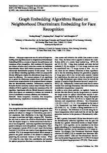
Figure 2: An illustration of the intuition behind Oriented Line Graph. Four nodes in two clusters are shown in the original graph, and edge weights, i.e., transition probabilities, are shown in the oriented line graph. If a walk from the yellow cluster randomly chooses to go to node (a → d), it must be followed by a series of walks inside the blue cluster, since backtracking is prohibited (indicated by the edge weight of 1), and vice versa. Moreover, structural hole spanners become more evident, as node (a → d) and node (d → a) are put into crucial positions with more concentrated edges weights.

Markovian process to a Markovian process by introducing an oriented line graph. Definition 3.3. (Oriented Line Graph) Given an undirected unweighted graph G = (V, E, A), its oriented ~ ·, P) is a directed weighted graph, line graph H = (E, whose node set is the set of oriented edges in G, and weighted adjacency matrix is the non-backtracking transition matrix.

Figure 2 illustrates the intuition behind the oriented line graph. It can be seen that the oriented line graph has the potential ability to characterize commuDefinition 3.2. (Non-Backtracking Transition nity boundary and emphasize structural hole spanners. Matrix) Given an undirected unweighted graph An intuitive graph embedding approach is to perform G = (V, E, A), we define its non-backtracking transition spectral decomposition on non-backtracking transition matrix P as a 2m × 2m matrix, which can be regarded matrix P. However, P is an asymmetric matrix, so it as a random walk on directed edges of graph G with is not guaranteed to have real eigenvalues and eigenbacktracking prohibited. Mathematically, vectors. Also, from the definition of P, some terms in (3.1)  P is invalid at dG (v) = 1, for v ∈ V . We propose the 1  , if v = x and u 6= y. Proposition 3.1 to make full use of P in spectral graph P[(u→v),(x→y)] = dG (v) − 1 embedding.  0, otherwise. Proposition 3.1. If the minimum degree of the conwhere u, v, x, y ∈ V and (u → v), (x → y) are edges nected graph G is at least 2, then the oriented line graph with directions taken into consideration. H is valid and strongly connected. By encoding a graph into a non-backtracking transition matrix, it allows the diffusion dynamics to be considered. Notice that, different from the original nonbacktracking operator [14], we also take the diffusion probability of the edges into account by the definition of P. In this way, it enables us to capture more information for complex topological structure of the graph. Further, non-backtracking random walk is a nonMarkovian chain, which uses non-backtracking transition matrix as its transition probability matrix. To make the analysis more tractable, we transform the non-

Proof. The proof is given in the Appendix A.1. Proposition 3.1 also means that under this condition the non-backtracking transition matrix P is irreducible and aperiodic. In particular, according to the Perron-Frobenius Theorem [11], it implies that for a strongly connected oriented line graph with nonnegative weights, matrix P has a unique left eigenvector φ with all entries positive. Let us denote r as the largest real eigenvalue of matrix P. Then, φT P = rφT .

For directed weighted graphs, nodes’ importance in topological structure is not determined by the degree of nodes as in an undirected graph, since directed edges coming in or going out of a node may be blocked or be rerouted back immediately in the next path. Hence, as discussed in lots of literatures [8], we use Perron vector φ to denote node importance in the oriented line graph. Our objective is to ensure that linked nodes in oriented line graph should be embedded into a close location in the embedding space. Suppose we want to embed nodes in the oriented line graph into one dimensional vector y. Regarding to each edge (e1 , e2 ) in the oriented line graph H, by considering its weights, our goal is to minimize (y(e1 ) − y(e2 ))2 P (e1 , e2 ). Taking source nodes’ importance indicated by φ into consideration and summing the loss over all edges, we define our loss function as X φ(e1 )[(y(e1 ) − y(e2 ))2 P (e1 , e2 )]. (3.2) min y

(e1 ,e2 )∈E(H)

Specifically, the Eq. (3.2) can be written in a matrix form by the following proposition. Proposition 3.2. Eq (3.2) has the following form (3.3)

min yT Ly, y

T

Proof. The proof is given in the Appendix A.2. Following the idea of [8], we consider the Rayleigh quotient for directed graphs as follows: yT Ly . yT Φy

The denominator of Rayleigh quotient takes the amount of weight distribution in the directed graph indicated by Φ into account. Therefore, we add yT Φy = 1 as a constraint, which can eliminate the arbitrary rescaling caused by y and Φ. By solving Eq. (3.3) with this constraint, we get the following eigenvector problem: (3.4)

Input: Graph G = (V, E); Embedding dimension k Output: Set of embedding vectors (y1 , y2 , · · · , yn ) 1: Preprocess original graph G to meet the requirement of Proposition 3.1 2: Initialize the non-backtracking transition matrix P by definition 3.2 3: Compute the second to the k + 1 smallest eigenT vectors of matrix Le = I − P+P , denoted by 2 g[1], g[2], · · · , g[k] 4: For every u ∈ V at every dimension i ∈ [1, · · · , k], P i.e., yu (i) = g[i]in u = v∈N (u) g[i]v→u , based on the in-sum rule. 5: return (y1 , y2 , · · · , yn ) Proposition 3.3. Both the sums of rows and columns of the non-backtracking transition matrix P equal one. That is, 1T P = 1T , where 1 is a column vector of ones. Proof. The proof is given in the Appendix A.3. From the Proposition 3.3, we know that P 1 is a Perron vector of P. By normalizing φ (subject to e φ(e) = 1), 1 ~ we can further have φ(e) = 2m for each node e ∈ E. Then, we have (3.5)

Φ is called combinatorial Laplawhere L = Φ − ΦP+P 2 cian for directed graphs, and Φ is a diagonal matrix with Φ(u, u) = φ(u).

R(y) =

Algorithm 1 NOBE: NOn-Backtracking Embedding

(Φ−1 L)y = λy.

e Φ−1 L = L, T

, and can be thought of as a where Le = I − P+P 2 normalized Laplacian matrix for oriented line graphs, compared to traditional Laplacian matrix for undirected T can be regarded as a symmetrication graphs. P+P 2 process on a 2m × 2m matrix. Specifically, this process will be equivalent to neutralize the weights between zero and P(e1 ,e2 ) if P(e1 ,e2 ) is not null, since P(e1 ,e2 ) and P(e2 ,e1 ) cannot be nonzero at the same time. According to Eq 3.4 and Eq 3.5, we could obtain k-dimensional embedding vectors of directed edges by e By computing k smallest non-trivial eigenvectors of L. summing these results over related embedding vectors, we can obtain node embeddings of graph G. Here we introduce two sum rules: in-sum and out-sum. Suppose we have got a one-dimensional vector of the embedding of edges denoted by g. For any P node u, we define the rule of in-sum by guin = v∈N (u) gv→u , which sums of all the incoming edges’ embeddings associated out with P u. We define the rule of out-sum by gu = v∈N (u) gu→v , which sums of all the outgoing edges’ embeddings associated with u. Our graph embedding algorithm is described in algorithm 1.

It is now clear that our task of this stage becomes selecting smallest eigenvectors of Φ−1 L to form a vector representation for directed edges from non-backtracking perspective. By using the following proposition, we can further reduce the Φ−1 L matrix into a more concise 3.3 Graph Approximation In the previous part, we present a spectral graph embedding algorithm and elegant form.

NOBE, which can preserve both macroscopic and microscopic structures of the original graph. The main procedure of NOBE uses a two-step operation sequentially: eigenvector decomposition and summation of incoming edge embeddings. The first step is conducted e which is equivalent to comon a 2m × 2m matrix L, T pute the several largest eigenvectors on P+P , denoted 2 as P. In this section, we will show how to speedup the algorithm by reversing these two steps. By graph approximation technique, we present an eigenvector decomposition algorithm acting on a 2n × 2n matrix with provable approximation guarantees. Suppose that g is an eigenvector of P of 2m dimensions on directed edges, then based on the definition of in-sum and out-sum, gin and gout are vectors of n dimensions after performing in-sum and out-sum operations. If these exists a 2n×2n matrix T and a 2m×2m matrix Q, such that !! ! ! (gT Q)in (gT P)in gin . ≈ = T (3.6) gout (gT Q)out (gT P)out This implies that if matrix Q adequately approximates P, without operating on matrix P , one can perform spectral decomposition directly on T, which is much smaller than P, to get gin and gout . We can view T as an aggregating version of matrix P, which means that T contains almost the same amount of information as P for our embedding purpose. Next, to compose T matrix, for any node u, we consider its out-sum operation when applying P matrix on it. Lemma 3.1. There exists a 2m × 2m matrix Q = P + ∆, such that for arbitrary node x, u, v ∈ V , 1 if P [(x→u),(u→v)] 6= |∆[(x→u),(u→v)] | ≤ 2(d(u)−1))(d(v)−1) 0, otherwise 0. Moreover, (gT P)out can be apu T out T out proximated as (g P) ≈ (g Q) = ( 21 − u u P P 1 1 1 in out v∈N (u) 2(d(v)−1) d(u) )gu + v∈N (u) 2(d(v)−1) gv . Proof. The proof is given in the Appendix A.5.

T in T P)in Likewise, operation, (gP u ≈ (g Q)u = P for in-sum 1 1 1 out in ( 12 − v∈N (u) 2(d(v)−1) )g + v∈N (u) 2(d(v)−1) gv . d(u) u After removing constant factors and transforming this formula into a matrix form, we have " # J I − D−1 J (3.7) T= , I − D−1 J J

directly selecting the second to the k + 1 largest eigenvectors of T as our embedding vectors. As these eigenvectors of 2n dimensions have in-sum and out-sum embedding parts, consistent with NOBE, we simply choose in-sum part as the final node embeddings. To prove the approximation guarantee of NOBEGA, we first introduce some basic notations from spectral graph theory. For a matrix A, we write A < 0, if A is positive semi-definite, Similarly, we write A < B, if A − B < 0, which is also equivalent to vT Av < vT Bv, for all v. For two graphs G and H with the same node set, we denote G < H if their Laplacian matrix LG < LH . Recall that xT LG x = P 2 (u,v)∈E WG (u, v)(x(u) − x(v)) , where WG (u, v) denotes an item in weighted adjacency matrix of G. It is clear that dropping edges will decrease the value of this quadratic form. Now, we define the approximation between two graphs based on the difference of their Laplacian matrices. Definition 3.4. (c-approximation graph) For some c > 1, a graph H is called a c-approximiation graph of graph G, if cH < G < H c . Based on the Definition 3.4, we present the Theorem 3.1, which further shows the relationship of G and its c-approximation graph H in terms of their eigenvalues. Theorem 3.1. If H is a c-approximation graph of graph G, then 1 |λk (G) − λk (H)| ≤ max{(c − 1), (1 − )}λk (G), c where λk (·) is the k-th smallest eigenvalue of the corresponding graph. Proof. The proof is given in the Appendix A.4. To relax the strict conditions in Definition 3.4, we define a probabilistic version of the c-approximation graph by using element-wise constraints. Definition 3.5. ((c, η)-approximation graph) For some c > 1, a graph H = (V, ·, WH ) is called a (c, η)-approximiation graph of graph G = (V, ·, WG )), if cWH (u, v) ≤ WG (u, v) ≤ 1c WH (u, v) is satisfied with probability at least 1 − η.

A probabilistic version of Theorem 3.1 follows accordingly. At last, we claim that matrix Q approximates matrix P well by the following Theorem, which means where I is the identity matrix and J = A(D − I)−1 . the approximation of NOBE-GA is adequate. By switching the order of spectral decomposition and summation, the approximation target is achieved. Now, Theorem 3.2. Suppose that the degree of the original our graph approximation algorithm NOBE-GA is just graph G obeys Possion distribution with parameter λ,

e = i.e., d ∼ π(λ). Then, for some small δ, graph H ~ (E, ·, Q) is a (c, η)-approximation graph of the graph ~ ·, P), where c is 1+δ, and η is 1 [ 1 + λ 3 ]. H = (E, δ λ−1 (λ−1) Proof. The proof is given in the Appendix A.6. 3.4 Time Complexity and Discussion A sparse implementation of our algorithm in Matlab is publicly available1 . For k-dimensional embedding, summation operation of NOBE requires O(mk) time. Eigenvector computation, which utilizes a variant of P Lanczos algorithm, requires O(e tk) time, where e t = v 2d(v)[d(v) − 1]. In total, the time complexity of NOBE is O(e tk+mk). The time complexity of NOBE-GA is O(nkd), where d is the average degree. Classic spectral method based on D−1 A is just a reduced version of NOBE (proof in Appendix A.7). For sparse and degree-skewed networks, nodes with a large degree will affect many related eigenvectors. Therefore, the previous leading eigenvector that corresponds to community structure will be lost in the bulk of worthless eigenvectors, and hence fail to preserve meaningful structures [14]. However, our spectral framework with non-backtracking strategy can overcome this issue. 4

Experimental Results

In this section, we first introduce datasets and compared methods used in the experiments. After that, we present empirical evaluations on clustering and structural hole spanner detection in detail. 4.1 Dataset Description All networks used here are undirected, which are publicly available on SNAP dataset platform [15]. They vary widely from a range of characteristics such as network type, network size and community profile. They include three social networks: karate (real), youtube (online), enron-email (communication); three collaboration networks: ca-hepth, dblp, ca-condmat (bipartite of authors and publications); three entity networks: dolphins (animals), us-football (organizations), polblogs (hyperlinks). The summary of the datasets is shown in Table 2. Specifically, we apply a community detection algorithm, i.e., RanCom [12], to show the detected community number and maximum community size.

Table 2: Summary of experimental datasets and their community profiles. Characteristics Datasets karate dolphins us-football polblogs ca-hepth ca-condmat email-enron youtube dblp

# Node 34 62 115 1,224 9,877 23,133 36,692 334,863 317,080

# Edge 78 159 613 19,090 25,998 93,497 183,831 925,872 1,049,866

#Community #Max members RankCom RankCom 2 18 3 29 11 17 7 675 995 446 2,456 797 3,888 3,914 15,863 37,255 25,633 1,099

• NOBE, NOBE-GA: Our spectral graph embedding method and its graph approximation version. • node2vec [9]: A feature learning framework extending Skip-gram architecture to networks. • LINE [26]: The version of combining first-order and second-order proximity is used here. • Deepwalk [21]: Truncated random walk and language modeling techniques are utilized. • HAM [10]: A harmonic modularity function is proposed to tackle the SH spanner detection. • Constraint [5]: A constraint introduced to prune nodes with certain connectivity being candidates. • Pagerank [20]: Nodes with highest pagerank score will be selected as SH spanners. • Betweenness Centrality (BC) [4]: Nodes with highest BC will be selected as SH spanners. • HIS [16]: Designing a two-stage information flow model to optimize the provided objective function. • AP BICC [23]: Approximate inverse closeness centralities and articulation points are exploited.

4.3 Performance on Clustering Clustering is an important unsupervised application used for automatically separating data points into clusters. Our graph embedding method is used for embedding nodes of a graph into vectors, on which clustering method can be directly employed. Two evaluation metrics considered are summarized as follows: • Modularity [18]: Modularity is a widely used quantitative metric that measures the likelihood of nodes’ community membership under the pertur4.2 Compared Methods We compare our methods bation of the Null model. Mathematically, Q = P d(v)·d(w) 1 with the state-of-the-art algorithms. The first three are ]δ(cv , cw ), where δ is the invw [Avw − 2m 2m graph embedding methods. The others are SH spanner dicator function. cv indicates the community node detection methods . We summarize them as follows: v belongs to. In practice, we add a penalty if a clearly wrong membership is predicted. 1 https://github.com/Jafree/NOnBacktrackingEmbedding

• Permanence [6]:

It is a vertex-based metric,

Table 3: Performance on Clustering evaluated by Modularity and Permanence(rank) Datasets

Clustering Methods k-means karate AM k-means dolphins AM k-means us-footbal AM k-means ca-hepTh AM k-means condmat AM k-means enron-email AM k-means polblogs AM

NOBE 0.449(1) 0.449(1) 0.510(2) 0.514(2) 0.610(2) 0.612(1) 0.639(1) 0.635(1) 0.515(1) 0.528(1) 0.219(2) 0.215(3) 0.428(1) 0.428(1)

NOBEGA 0.449(1) 0.449(1) 0.522(1) 0.522(1) 0.611(1) 0.609(2) 0.609(2) 0.614(2) 0.495(3) 0.502(3) 0.221(1) 0.220(1) 0.428(1) 0.427(2)

Modularity node2vec LINE 0.335(5) 0.335(4) 0.460(3) 0.458(3) 0.605(3) 0.589(3) 0.597(3) 0.606(3) 0.515(1) 0.520(2) 0.213(3) 0.218(2) 0.357(3) 0.376(3)

0.403(3) 0.239(5) 0.187(5) 0.271(5) 0.562(4) 0.492(4) 0.01(5) 0.05(5) 0(5) 0(5) 0(5) 0(5) 0.200(4) 0.266(4)

which depends on two factors: internal clustering coefficient and maximum external degree to other communities. The permanence of a node v that belongs to community c is defined as follows: 1 c P ermc (v) = [ E cIc (v)(v) × d(v) ] − [1 − Cin (v)], where max c Ic (v) is the internal degree. Emax (v) is the maximum degree that node v links to another comc (v) is the internal clustering coeffimunity. Cin cient. Generally, positive permanence indicates a good community structure. To penalize apparently wrong community assignment, P ermc (v) is set to c −1, if d(v) < 2Emax (v). For the clustering application, we summary the performance of our methods, i.e., NOBE and NOBE-GA, against three state-of-the-art embedding methods on seven datasets in terms of modularity and permanence in Table 3. Two types of classic clustering methods are used, i.e., k-means and agglomerative method (AM). From these results, we have the following observations: • In terms of modularity and permanence, NOBE and NOBE-GA outperform other graph embedding methods over all datasets under both k-means and AM. Positive permanence scores on all datasets in-

Modularity

Permanence

3.5 karate dolphins us-football ca-hepth ca-condmat enron-email polblog

1.75

3.0

1.50 2.5 1.25 2.0 1.00 1.5 0.75 1.0

0.50

0.5

k-means AM

0.25

0.0

0.00 NOBE

NOBE-GA node2vec

LINE

Deepwalk

NOBE

NOBE-GA

node2vec

Deepwalk

Figure 3: The overall performance on clustering in terms of modularity and permanence.

Deepwalk 0.396(4) 0.430(3) 0.401(4) 0.393(4) 0.464(5) 0.464(5) 0.424(4) 0.453(4) 0.357(4) 0.370(4) 0.178(4) 0.207(4) 0.084(5) 0.065(5)

NOBE 0.350(1) 0.356(1) 0.250(2) 0.233(2) 0.321(1) 0.330(1) 0.412(1) 0.435(1) 0.330(1) 0.391(1) 0.096(2) 0.120(3) 0.138(1) 0.138(1)

NOBEGA 0.350(1) 0.350(2) 0.268(1) 0.249(1) 0.321(1) 0.330(1) 0.337(3) 0.416(2) 0.288(3) 0.327(3) 0.153(1) 0.194(1) 0.136(2) 0.132(2)

Permanence node2vec LINE

Deepwalk

0.335(4) 0.205(5) 0.196(3) 0.132(4) 0.304(3) 0.279(4) 0.379(2) 0.406(3) 0.330(1) 0.388(2) 0.080(3) 0.180(2) -0.066(3) -0.096(3)

0.350(1) 0.311(3) 0.187(4) 0.189(3) 0.039(5) 0.039(5) 0.261(4) 0.338(4) 0.197(4) 0.249(4) 0.049(4) 0.108(4) -0.187(4) -0.176(4)

0.182(5) 0.232(4) -0.166(5) -0.189(5) 0.311(2) 0.307(3) -0.948(5) -0.949(5) -0.984(5) -0.994(5) -0.985(5) -0.996(5) -0.569(5) -0.509(5)

dicate that meaningful community structure is discovered. Specifically, node2vec obtains competing results on condmat under k-means. As for LINE, it fails to predict useful community structure on most large datasets except karate and us-football. Deepwalk gives mediocre results on most datasets and bad results on us-football, polblogs and enron-email under k-means. • Figure 3 reports the overall performance. NOBE and NOBE-GA achieves superior embedding performance for the clustering application. Moreover, it practically demonstrates that NOBE-GA approximates NOBE very well on various kinds of networks despite the difference on their link density, node preferences and community profiles. To our surprise, on some datasets NOBE-GA even achieve slightly better performance than NOBE. We conjecture that this improvement arises because of the introducing of the randomization and the preferences of evaluation metrics. Specifically, in terms of modularity, the percentage of improvement margin of NOBE is 8% over node2vec, 139% over LINE and 39% over Deepwalk. Regarding to permanence, the percentage of the improvement margin of NOBE is 16% over node2vec and 100% over Deepwalk. 4.4 Performance on Structural Hole Spanner Detection Generally speaking, in a network, structural hole (SH) spanners are the nodes bridging between different communities, which are crucial for many applications such as diffusion controls, viral marketing and brain functional analysis [2, 16, 5]. Detecting these bridging nodes is a non-trivial task. To exhibit the power of our embedding method in placing key nodes into accurate positions, we first employ our method to embed the graph into low-dimensional vectors and then detect structural hole spanners in that subspace. We compare our method with SH spanner detection algo-

Table 4: Structural hole spanner detection results under linear threshold and independent cascade influence models

youtube

78

dblp

42

Comparative Methods HAM Constraint PageRank 0.343 0.295 0.159 0.002 0.002 0.001 [3 20 9] [1 34 3] [34 1 33] 3.951 2.447 1.236 2.452 1.254 0.662 5.384 0.404 0.357 3.578 0.229 0.190

rithms that are directly applied on graphs. To evaluate the quantitative quality of selected SH spanners, we use a evaluation metric called Structural Hole Influence Index (SHII) proposed in [10]. This metric is designed by simulating information diffusion processes under certain information diffusion models in the given network. • Structural Hole Influence Index (SHII) [10]: Regarding a SH spanner candidate v, we compute its SHII score by performing the influence maximization process several times. For each time, to activate the influence diffusion process, we randomly select a set of nodes Sv from the community Cv that v belongs to. Node v and node set Sv is combined as seed set to propagate the influence. After the propagation, SHII score is obtained by computing the relative difference between the number of activated nodes in the community Cv and P in other communities: SHII(v, Sv ) = P Ci ∈C\Cv P

u∈Ci

Iu

, where C is the set of communities. Iu is the indicator function which equals one if node u is influenced, otherwise 0. For each SH spanner candidate, we run the information diffusion under linear threshold model (LT) and independent cascade model (IC) 10000 times to get average SHII score. To generate SH spanner candidates from embedded subspace, in which our embedding vectors lie, we devise a metric for ranking nodes: u∈Cv

Iu

• Relative Deviation Score (RDS): Suppose that for each node v ∈ V , its low-dimensional embedding vector is represented as yv ∈ Rk . We apply k-means to separate nodes into appropriate clusters with C denoting cluster set. For a cluster C ∈ C, 1 P the mean of its points is uC = |C| i∈C yi . The Relative Deviation Score, which measures how far a data point is deviating from its own community attracted by other community, is defined as: RDS(v) = max C∈C

k yv − uCv k2 /RCv k yv − uC k2 /RC

where P Cv denotes the cluster v belongs to. And RC = i∈C k yi − uC k2 indicates the radius of

BC 0.159 0.001 [1 34 33] 1.226 0.791 0.958 0.821

HIS 0.132 0.001 [32 9 14] 3.198 2.148 0.718 0.304

AP BICC 0.295 0.002 [1 3 34] 1.630 0.799 0.550 0.495

cluster C. In our low-dimensional space, nodes with highest RDS will be selected as candidates of SH spanners. We summarize our embedding method against other SH spanner detection algorithms in Table 4. Due to space limit, we omit the results of other embedding methods as they totally fail on this task. The number of SH spanners shown in the second column is chosen based on the network size and community profile. Actually, too many SH spanners will lead to the propagation activating the entire network. We outperform all SH spanner detection algorithms under LT and IC models on all three datasets. Specifically, on karate network, we identify three SH spanners, i.e., 3, 20 and 14, which can be regarded as a perfect group that can influence both clusters, seen from Figure 1. On average, our method NOBE achieves a significant 66% improvement against state-of-the-art algorithm HAM, which shows the power of our method in accurate embedding.

0.6 0.2

0.5 0.4

Permanence

3

NOBE 0.595 0.003 [3 20 14] 4.664 4.375 8.734 7.221

0.3 0.2

NOBE NOBE-GA node2vec LINE deepwalk

0.1 0.0

0

5

10

15

20

Dimension

25

0.0

−0.2 NOBE NOBE-GA node2vec LINE deepwalk

−0.4

−0.6 30

0

5

10

15

20

Dimension

25

30

(a) us-football 0.4

0.6

0.2

0.5

0.0

0.4

NOBE NOBE-GA node2vec LINE deepwalk

0.3 0.2

Permanence

karate

Influence Model LT IC SH spanners LT IC LT IC

Modularity

#SH Spanners

Modularity

Datasets

NOBE NOBE-GA node2vec LINE deepwalk

−0.2 −0.4 −0.6 −0.8

0.1

−1.0 0.0 0

25

50

75

100

Dimension

125

150

175

200

−1.2

0

25

50

75

100

Dimension

125

150

175

200

(b) ca-hepth Figure 4: Parameter Analysis of Dimension under AM.

4.5 Parameter Analysis Dimension is usually considered as a intrinsic characteristic, and often needs to be artificially predefined. With varying dimension, we report the clustering quality under AM on two datasets in Figure 4. On football network with 11 ground truth communities, NOBE, NOBE-GA and node2vec achieves reasonable results on dimension k = 7 or 8. After k = 11, NOBE, NOBE-GA, node2vec and deepwalk begin to drop. Followed by a sudden drop, node2vec still increases gradually. Reported by RankCom, ca-hepth network has 995 communities. Nevertheless, prior to dimension k = 50, NOBE, NOBE-GA, node2vec and deepwalk have already obtained community structure with good quality. The performance will slightly increase afterwards. Consistent with studies on spectral analysis of graph matrices [25], community number is a good choice for dimension. However, it’s also rather conservative, since good embedding methods could preserve great majority of graph information in much shorter vectors. The choice of a large number greater than community number should be cautious since redundant information added may deteriorate embedding results . 5 Conclusion and Outlook This paper proposes NOBE, a novel framework leveraging the non-backtracking strategy for graph embedding. It exploits highly nonlinear structure of graphs by considering a non-Markovian dynamics. As a result, it can handle both macroscopic and microscopic tasks. Experiments demonstrate the superior advantage of our algorithm over state-of-the-art baselines. In addition, we carry out a graph approximation technique with theoretical guarantees for reducing the complexity and also for analyzing the different flows on graphs. To our surprise, NOBE-GA achieves excellent performance at the same level as NOBE. We hope that our work will shed light on the analysis of algorithms based on flow dynamics of graphs, especially on spectral algorithms. Graph approximation can be further investigated by considering the perturbation of eigenvectors. We leave it for future work.

[2]

[3]

[4] [5] [6]

[7] [8] [9] [10]

[11] [12]

[13]

[14]

[15]

[16]

[17]

Acknowledgement This work is supported in part by National Key R& D Program of China through grants 2016YFB0800700, and NSF through grants IIS-1526499, and CNS1626432, and NSFC 61672313, 61672051, 61503253, and NSF of Guangdong Province 2017A030313339.

[18]

References

[21]

[1] S. Abu-El-Haija, B. Perozzi, and R. Al-Rfou,

[19]

[20]

[22]

Learning edge representations via low-rank asymmetric projections, arXiv:1705.05615, (2017). D. S. Bassett, E. T. Bullmore, A. MeyerLindenberg, J. A. Apud, D. R. Weinberger, and R. Coppola, Cognitive fitness of cost-efficient brain functional networks, PNAS, (2009). C. Bordenave, M. Lelarge, and L. Massouli´ e, Non-backtracking spectrum of random graphs: community detection and non-regular ramanujan graphs, in FOCS, 2015. U. Brandes, A faster algorithm for betweenness centrality, Journal of mathematical sociology, (2001). R. S. Burt, Structural holes: The social structure of competition, Harvard university press, 2009. T. Chakraborty, S. Srinivasan, N. Ganguly, and S. Bhowmick, On the permanence of vertices in network communities, in KDD, 2014. M. Chen, Q. Yang, and X. Tang, Directed graph embedding., in IJCAI, 2007. F. Chung, Laplacians and the cheeger inequality for directed graphs, Annals of Combinatorics, (2005). A. Grover and J. Leskovec, node2vec: Scalable feature learning for networks, in KDD, 2016. L. He, C.-T. Lu, J. Ma, J. Cao, L. Shen, and P. S. Yu, Joint community and structural hole spanner detection via harmonic modularity, in KDD, 2016. R. A. Horn and C. R. Johnson, Matrix analysis, Cambridge university press, 2012. F. Jiang, Y. Yang, S. Jin, and J. Xu, Fast search to detect communities by truncated inverse page rank in social networks, in ICMS, 2015. M. Kempton, High Dimensional Spectral Graph Theory and Non-backtracking Random Walks on Graphs, University of California, San Diego, 2015. F. Krzakala, C. Moore, E. Mossel, J. Neeman, ´ , and P. Zhang, Spectral reA. Sly, L. Zdeborova demption in clustering sparse networks, PNAS, (2013). J. Leskovec and A. Krevl, SNAP Datasets: Stanford large network dataset collection. http://snap.stanford.edu/data, 2014. T. Lou and J. Tang, Mining structural hole spanners through information diffusion in social networks, in WWW, 2013. F. Morone and H. A. Makse, Influence maximization in complex networks through optimal percolation, Nature, (2015). M. E. Newman, Modularity and community structure in networks, PNAS, (2006). M. Ou, P. Cui, J. Pei, Z. Zhang, and W. Zhu, Asymmetric transitivity preserving graph embedding, in KDD, 2016. L. Page, S. Brin, R. Motwani, and T. Winograd, The pagerank citation ranking: Bringing order to the web., tech. report, Stanford InfoLab, 1999. B. Perozzi, R. Al-Rfou, and S. Skiena, Deepwalk: Online learning of social representations, in KDD, 2014. H. Qiu and E. R. Hancock, Clustering and embed-

ding using commute times, TPAMI, (2007). [23] M. Rezvani, W. Liang, W. Xu, and C. Liu, Identifying top-k structural hole spanners in large-scale social networks, in CIKM, 2015. ´ , Spec[24] A. Saade, F. Krzakala, and L. Zdeborova tral density of the non-backtracking operator on random graphs, EPL, (2014). [25] H.-W. Shen and X.-Q. Cheng, Spectral methods for the detection of network community structure: a comparative analysis, Journal of Statistical Mechanics: Theory and Experiment, (2010). [26] J. Tang, M. Qu, M. Wang, M. Zhang, J. Yan, and Q. Mei, Line: Large-scale information network embedding, in WWW, 2015. [27] D. Wang, P. Cui, and W. Zhu, Structural deep network embedding, in KDD, 2016. [28] L. Xu, X. Wei, J. Cao, and P. S. Yu, Embedding of embedding (eoe): Joint embedding for coupled heterogeneous networks, in WSDM, 2017.

A Appendix A.1 Proposition 3.1 If the minimum degree of the connected graph G is at least 2, then the oriented line graph H is valid and strongly connected.

Proposition 3.2 Our loss function is

A.2

min yT (Φ − y

ΦP + PT Φ )y. 2

Proof. To be concise, we use V (H), E(H) denote the node set and the edge set of H separately. u,v denote nodes in V (H). Considering every node pair, we have the following loss function X

{φ(u)[(y(u)−y(v))2 P (u, v)]+φ(v)[(y(v)−y(u))2P (v, u)]}.

u,v∈V (H)

Dividing the term into two parts by regarding each node pair as ordered and expanding the formula, we get (A.1) 1 X 2

X

X

X

[φ(u)(y(u)2 + y(v)2 − 2y(u)y(v))P (u, v)]

u∈V (H) (u,v)∈E(H)

1 + 2

[φ(v)(y(u)2 + y(v)2 − 2y(u)y(v))P (v, u)]

u∈V (H) (v,u)∈E(H)

Then, we do the deduction for the first part. A similar proof can be applied to the second part. Enumerating each node in the first part, we get X 1 X p(u, v) φ(u)y(u)2 2 u∈V (H)

Proof. Assume that (w → x) and (u → v) are two arbitrary nodes in the oriented line graph H. The proposition is equivalent to prove that (u → v) can be reached from (w → x). Three situations should be considered: 1) if x = u and w 6= v, then (w → x) is directly linked to (u → v); 2) if w = v and x 6= u which means there is a directed edge from (u → v) to (w → x). We delete the node w, i.e., node v, in the original graph G. Since the minimum degree of G is at least two. Therefore, node u and node x are still mutually reachable in graph G. A Hamilton Path p from node x to node u can be selected with passing through other existing nodes only once, which satisfies the non-backtracking condition. Adding node w, i.e., node v, back into the graph G will generate a non-backtracking path (w → p → v), which means (u → v) is reachable from (w → x) in the oriented line graph H; 3) if w, x, u, v are mutually unequal. Assume that we delete edges (w, x) and (u, v) in graph G, then graph G is still connected. There exists a Hamilton path p connecting node x and u. Thus, with (w → p → v) satisfying the non-backtracking condition, there exists a directed path connecting node (w → x) and node (u → v) in the oriented line graph H. Overall, every valid node in graph H can be reached, if graph G has a minimum degree at least two.

(A.2)

1 + 2

−

1 2

X

v:(u,v)∈E(H)

y(v)2

v∈V (H)

X

X

(φ(u)P (u, v))

u:(u,v)∈E(H)

φ(u)(2y(u)y(v)P (u, v))

v:(u,v)∈E(H)

Due to proposition 3.3, the sum of each row is equal to one, i.e., X P (u, v) = 1. v:(u,v)∈E(H)

The first part of above equation becomes 1 T y Φy. 2

Here, Φ is a diagonal matrix with Φ(i, i) = φ(i). Since φT P = φT , so the second sum in the second term of equation A.2 becomes X (φ(u)P (u, v)) = φ(v). u:(u,v)∈E(H)

Then, the matrix form of the second term in equation A.2 becomes 1 T y Φy 2 Arranging the terms in a particular order, we can easily see the third part in equation A.2 X 1 2y(u)φ(u)P (u, v)y(v) = yT ΦPy. − 2 v:(u,v)∈E(H)

Adding up all terms and removing the constant factor, A.5 Lemma 3.1 There exists a 2m × 2m matrix we get our loss function Q = P + ∆, such that for arbitrary node x, u, v ∈ V , if P [(x→u),(u→v)] 6= 0, then |∆[(x→u),(u→v)] | ≤ 1 T out ΦP + PT Φ T can 2(d(u)−1))(d(v)−1) otherwise 0. Moreover, (g P)u )y. min y (Φ − y 2 1 T out T out be approximated as (g P) ≈ (g Q) = ( u u 2 − P P 1 1 1 in out )g + g . v∈N (u) 2(d(v)−1) v v∈N (u) 2(d(v)−1) d(u) u A.3 Proposition 3.3 Both the sums of rows and columns of the non-backtracking transition matrix P Proof. Considering the vector g as the information conequal one. tained on each directed edge in graph G, from the defiProof. The proof is simple, since concerning each row nition of out operation and the non-backtracking tranT out or column, the values of nonzero items are equal. For sition matrix, (g P)u is equivalent to a process that an arbitrary row related to node (u → v), the sum of first applying one step random walk with probability transition matrix P to update the vector g, and then this row in the non-backtracking matrix P is conducting out operation on node u in graph G. So, we X X 1 can get P[(u→v),(v→x)] = (A.4) d(v) − 1 X x∈N (v) x6=u

x∈N (v) x6=u

=

(gT P)out = u

X 1 1=1 d(v) − 1

(gT P)u→v

v∈N(u)

X

=

x∈N (v) x6=u

X

(

v∈N(u) x∈N(u) x6=v

1 gx→u + 2(d(u) − 1)

X y∈N(u) y6=u

1 gv→u ) 2(d(v) − 1)

Similarly, we can get the same result for each column.

For the first part in the second equation of equation A.4, by separating the non-backtracking part and switching the summation we have

A.4 Theorem 3.1 If G and H are graphs such that H is a c-approximation graph of graph G, then

(A.5) X

1 |λk (G) − λk (H)| ≤ max{(c − 1), (1 − )}λk (G), c where λk is the k-th smallest eigenvalue of corresponding graph.

X

v∈N(u) x∈N(u) x6=v

X

=

λk (G) =

minn max

x∈S S⊆R dim(S)=k

xT LG x . xT x

X

(

v∈N(u) x∈N(u)

X

=(

v∈N(u)

Proof. Applying Courant-Fisher Theorem, we have

1 gx→u 2(d(u) − 1) 1 1 gx→u − gv→u ) 2(d(u) − 1) 2(d(u) − 1

X X 1 1 gx→u − ) gv→u 2(d(u) − 1) 2(d(u) − 1 x∈N(u)

v∈N(u)

d(u) 1 =( − )guin 2(d(u) − 1) 2(d(u) − 1) 1 = guin 2

For the second part of equation A.4, we have As H is a c-approximation graph of G, then LG < 1c ·LH . (A.6) X X 1 So, we have gv→u 2(d(v) − 1) 1 T v∈N(u) y∈N(u) T x LG x ≥ x LH x. y6=u c X X 1 = gv→y Then, it becomes to 2(d(v) − 1) v∈N(u) y∈N(v) (A.3) y6=u 1 T xT LG x X c x LH x 1 λk (G) = minn max ≥ minn max (gvout − gv→u ) = x∈S x∈S S⊆R S⊆R xT x xT x 2(d(v) − 1) dim(S)=k

=

1 c

minn max

x∈S S⊆R dim(S)=k

v∈N(u)

dim(S)=k

T

1 x LH x = λk (H). T x x c

≈

X

v∈N(u)

X 1 1 1 in g out − g 2(d(v) − 1) v 2(d(v) − 1) d(u) u v∈N(u)

The approximation in the third step adopts an idea from Similarly, we can get cλk (H) ≥ λk (G). In other words, mean field theory that we assume that every incoming cλk (G) ≥ λk (H) ≥ 1c λk (G). Easy math will give the edge to a fixed node has the same amount of probability. final result. Thus, to give an unbiased estimation, we use the mean

1 (guin − Taylor series expansion around E[X]: of other edges coming into node u, i.e., d(u)−1 gv→u ), to approximate the gv→u when going through (A.7) (v → u) is prohibited by non-backtracking strategy. E[Y ] = E[ 1 ] ≤E{ 1 − 1 (X − E[X]) X E[X] E 2 [X] Note that for a neighbor x ∈ N (v), P[(x→v,v→u)] ≤ 1 1 2(d(v)−1) . By above approximation, matrix Q is ob+ 3 (X − E[X])2 } E [X] tained with Q = P + ∆, and the bound of the approx1 E 2 [X] + V ar[X] . To imation error is |∆[(x→v,v→u)] | ≤ 2(d(v)−1)(d(u)−1) = E 3 [X] sum up equation A.5 and A.6, we have (λ − 1)2 + λ X 1 1 1 (Due to Possion distribution) = T out )g in (gT P)out (λ − 1)3 u ≈ (g Q)u = ( − 2 2(d(v) − 1) d(u) u v∈N (u) λ 1 + = X 1 λ − 1 (λ − 1)3 + g out 2(d(v) − 1) v v∈N (u) So the upper bound that the relative difference ratio between corresponding elements in P and Q, which is The lemma holds. caused by the approximation, is as follows: A.6 Theorem 3.2 Suppose that the degree of the 1 1 1 λ original graph G obeys Possion distribution with paP r[ ). ≥ δ] ≤ ( + d(v) − 1 δ λ − 1 (λ − 1)3 rameter λ, i.e., d ∼ π(λ). Then, for arbitrary small e = (E, ~ ·, Q) is a (c, η)-approximation graph δ, graph H e is (1 + δ, η)~ ·, P), where c is 1 + δ, and η is Set η = 1 [ 1 + λ 3 ]. Then, graph H of the graph H = (E, δ λ−1 (λ−1) 1 1 λ approximation graph of graph H. δ [ λ−1 + (λ−1)3 ].

Claim 1 Spectral method based on lazy random e and A.7 Proof. To investigate the relationship between H walk is a reduced version of our proposed algorithm H, we first consider the relative difference between P NOBE. and Q. According to lemma 3.1, for an arbitrary nonzero item P[(x→u),(u→v)] in P, we have Proof. The proof is similar to Lemma 3.1. The detail of the approximation strategy used here is differ1 . P[(x→u),(u→v)] = ent. Again, regarding the vector g as the information 2(d(u) − 1) contained on each directed edge in graph G, (gT P)out u The maximum value of the corresponding item in ∆ is is equivalent to a process that first applying one step random walk with probability transition matrix P to 1 update the vector g, and then conducting out operation . |∆[(x→u),(u→v)] | = 2(d(v) − 1)(d(u) − 1) on node u in graph G. So, we can get So, the relative difference between P and Q is |∆[(x→u),(u→v)] | P[(x→u),(u→v)]

=

1 . d(v) − 1

(A.8) (gT P)out = u

X

(gT P)u→v

v∈N(u)

X

=

X

(

v∈N(u) x∈N(u) x6=v

1 gx→u + 2(d(u) − 1)

X y∈N(u) y6=u

1 gv→u ) 2(d(v) − 1)

Due to the arbitrary choice of node u and v, we regard For the first part in the second equation of equation A.8, the values concerning u and v as random variables. by separating non-backtracking part and switching the Thus, after applying Markov inequality, we get summation we have P r[

1 1 1 ≥ δ] ≤ E[ ]. d(v) − 1 δ d(v) − 1

Note that due to the convexity of the reciprocal function, applying Jensen’s inequality only gives us the lower 1 ], we set ranbound. To get an upper bound of E[ d(v)−1 1 dom variable X = d(v) − 1 and Y = X , one can use the

(A.9) X

X

v∈N(u) x∈N(u) x6=v

=(

X

v∈N(u)

1 = guin 2

1 gx→u 2(d(u) − 1)

X X 1 1 gx→u − ) gv→u 2(d(u) − 1) 2(d(u) − 1 x∈N(u)

v∈N(u)

For the second part of equation A.8, we have (A.10) X

X

v∈N(u) y∈N(u) y6=u

=

X

v∈N(u)

=

X v∈N(u)

≈

X

v∈N(u)

=

X v∈N(u)

1 gv→u 2(d(v) − 1)

X 1 gv→y 2(d(v) − 1) y∈N(v) y6=u

1 (gvout − gv→u ) 2(d(v) − 1) X 1 1 1 out gvout − g 2(d(v) − 1) 2(d(v) − 1) d(v) v v∈N(u)

X 1 d(v) − 1 g out = g out 2(d(v) − 1)d(v) v 2d(v) v v∈N(u)

The approximation happened on the third step of 1 gvout to approximate the above equation by using d(v) gv→u . This approximation is straightforward, since it allows one to diffuse information without inspecting the information collecting from which node. To sum up equation A.9 and equation A.10, we have X 1 1 in (gT P)out g out u ≈ gu + (A.11) 2 2d(v) v v∈N (u)

Likewise, we can get (A.12)

(gT P)in u ≈

X

v∈N (u)

1 1 g in + guout 2d(v) v 2

Assume that R is a 2n by 2n matrix, such that ! !! (gT P)in gin (A.13) = R gout (gT P)out This implies that if this equation holds, under the approximation described above, the spectral method is reduced from a spectral decomposition on the 2m × 2m matrix P to that on the 2n × 2n matrix R by dropping and approximating some information. According to equation A.13, we organize equation A.11 and A.13 into a matrix form, we get " −1 # D A I (A.14) R= , I D−1 A where I is the identity matrix. Literally, eigenvector decomposition on R and then selecting values corresponding to in component is equivalent to a conventional spectral method on lazy random walk. We set T T yT = (yin , yout ) as an eigenvector of matrix R with eigenvalue λ. Then, it becomes ( yout + D−1 Ayin = λyin (A.15) yin + D−1 Ayout = λyout

Consider two situations: 1)If yin = yout , substituting yout using yin into the first equation of the equation A.15, we obtain (D−1 A + I)yin = λyin , where B = 21 D−1 A + 21 I is the transition probability matrix of lazy random walk, which has the same eigenvectors with the transition probability matrix on classic random walk. Therefore, the eigenvectors of the transition probability matrix of the lazy random walk are contained in the in part of the eigenvectors of matrix R. 2)If yin 6= yout , substituting yout from the first equation of equation A.15 into the second equation, we get (A.16)

(λ2 I + (D−1 A)2 − 2λD−1 A − I)yin = 0.

The solution of equation A.16 is the root of (A.17)

det[λ2 I + (D−1 A)2 − 2λD−1 A − I] = 0,

where det is short for determinant. Equation A.17 has the similar form as the well-known graph zeta function det[λ2 I + D − λA − I] = 0, which facilitates many crucial problems on graphs. We argue that our framework can offer great opportunities to explore flow dynamics on graphs. This proof shows the flexibility of our framework NOBE and the applicability of graph approximation technique. Spectral decomposition algorithm based on lazy random walk is a reduced version of our proposed algorithm NOBE. The claim holds.