On Stochastic Controller Placement in Software-defined Wireless ...

On Stochastic Controller Placement in Software-defined Wireless Networks Mohammad J. Abdel-Rahman1 , EmadelDin A. Mazied2,3 , Allen MacKenzie1 , Scott Midkiff1 , Mohamed R. Rizk3 , and Mustafa El-Nainay4 1

Electrical and Computer Engineering Department Virginia Tech, USA

2

Electrical Engineering Department Sohag University, Egypt

Abstract— Software-defined networking (SDN) abstracts and centralizes the network control functions in a software entity that runs on a server, known as SDN controller. The controller needs to respond to its controlled elements in a strictly timely manner, and the controller placement has a prominent effect on its response time. Originally, all SDN architectures assumed a physical wired connection between the SDN controller and its controlled elements, and the controller placement problem (CPP) has been only studied under such wired settings. Recently, novel SDN architectures have been proposed in which a direct wireless connection is assumed between the controller and its controlled elements. In this paper, we consider the ‘wireless CPP,’ when the link between the controller and the controlled element is wireless. Specifically, our contributions are as follows. First, we propose two joint controller placement and assignment formulations, assuming wired links between the controllers and their controlled elements; the first formulation considers an average response time constraint, whereas the second one considers a per-link response time constraint. Then, using chanceconstrained stochastic programming (CCSP), we extend our formulation to the case when the links between the controllers and their controlled elements are wireless. Finally, we evaluate our joint placement and assignment schemes under various system parameters. Our results demonstrate the advantage of our joint scheme, in terms of reducing the required number of controllers, compared to a recent sequential assignment and placement scheme in the literature. They also show the ability of our CCSP-based scheme in probabilistically satisfying the controllers response time constraints.

I. I NTRODUCTION Software-defined networking (SDN) abstracts and centralizes the network control functions in a software entity that runs on a server that is known as an SDN controller [1]. Recently, SDN has been extended to include the wireless radio access network (RAN) control functionalities in many wireless architectures [2]. Robust and efficient control plane design is required to conquer the complexity of these proposed architectures of software-defined wireless networks (SDWN). The SDN controller is the key resource element in the network control plane design. It interacts with each network entity through controlling the infrastructure layer to provide This material is based upon work supported by the National Science Foundation under Grant No. 1443978.

3

Electrical Engineering/4 Computer & Systems Engineering Department Alexandria University, Egypt

a robust and flexible network management framework. This control process is carried out through logical communication design, e.g., OpenFlow [1], HyperFlow [3], CrossFlow [4], and physical communication. The controller communicates with the infrastructure network elements using either wired or wireless connection [5], [6]. To provide more flexible designs, recent advances in SDWN architectures assume wireless connectivity between the controller and the controlled element [5], [6]. Such wireless connectivity has drawn a significant attention from the researchers to develop a direct logical connectivity between the controller and its associated elements. For example, the authors in [4] developed a prototype of wireless node, using Xilinx-Artix software radio platform, with embedded soft-switch agent to enable a direct wireless communication between the wireless node and the controller. As SDN controllers play a crucial role, they need to respond to their associated nodes in a strictly timely manner (within a few milliseconds). Optimal placement of SDN controllers has a prominent effect on minimizing such response time. Distributing a minimum number of controllers at optimal locations to proceed the control functions in a strictly timely manner is known as the controller placement problem (CPP). CPP is well studied in wired networks (examples include [7]– [10]) using different objectives and constraints that are related to the network latency, reliability, and load balancing. In [11], [12], the authors studied the CPP in wireless dense networks. They developed a flow-based optimal controller placement mechanism with dynamic base station-controller assignment. Yet indelible mark of recent CPP models in SDWN, the work in [11], [12] assumes wired connectivity between the controller and the wireless base station. To the best of our knowledge, all proposed CPP models in the literature assume physical wired connections between the SDN controllers and their controlled elements. Our Contributions–In this paper, we consider the ‘wireless CPP,’ when the link between the controller and the controlled element is wireless. Specifically, the main contributions of this paper can be summarized as follows: • First, we consider the joint controller placement and

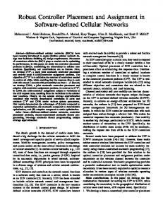
assignment problem assuming wired links between the controllers and their controlled elements. We propose two formulations of this problem considering two different QoS metrics. In the first formulation, we constrain the average response time of each controller (averaged over all nodes assigned to a given controller) to be less than a predetermined value δ. In the second formulation, we constrain the maximum response time of each controller to be less than δ across all of its assigned nodes. • Then, using chance-constrained stochastic programming (CCSP), we extend our formulation to the case when the links between the controllers and their controlled elements are wireless. Stochastic programming provides a powerful mathematical tool to handle optimization under various sources of uncertainty. It has been recently exploited to optimize resource allocation in various types of wireless networks operating under uncertainties (examples include [13]–[17]). • Finally, we evaluate our joint placement and assignment schemes under various system parameters. When the links are assumed to be wired, we evaluate our schemes using the network topologies in [18], and compare them with [10]. Our scheme for wireless links is evaluated on the grid network topology used in [11]. Paper Organization–The rest of the paper is organized as follows. We describe our system model and state our problem in Section II. Two variants of the joint placement and assignment problem when links are wired are formulated in Section III. We formulate the stochastic joint placement and assignment problem for wireless links in Section IV. All proposed formulations are numerically evaluated in Section V. Finally, we conclude the paper in Section VI. II. S YSTEM M ODEL AND P ROBLEM S TATEMENT We consider a set S = {1, 2, . . . , S} of controlled elements deployed in a geographical area, which contains a set C = {1, 2, . . . , C} of candidate locations for deploying SDN controllers. The SDN controllers will be connected to the controlled elements through wireless links. Each controlled element will have an embedded soft-switch agent with a wireless interface to communicate directly with the controller. A simplified view of our adopted architecture is depicted in Figure 1. As an example, Figure 1 presents a cellular network controlled by a set of SDN controllers, however, our study is not restricted to cellular network architectures. As illustrated in Figure 1, each wireless link, say between controller c and controlled element s, is associated with probability psc , which is the probability of successful transmission over this link. psc depends on the assumed wireless channel model. As an example, our results in Section V are obtained assuming a combined path loss and shadowing model, under which psc is given by [19]: ) ( Pmin − (Pt + 10 log10 k − 10 γ log10 (d/d0 )) psc = Q σψdB (1)

Fig. 1: SDN controller connection to infrastructure elements. where Q(·) is the Q-function, Pmin is the minimum received power below which an outage occurs (in dBm), Pt is the transmitted power (in dBm), k is a unitless constant that depends on the antenna characteristics and the average channel attenuation, γ is the path-loss exponent, d is the distance between controller c and controlled element s, d0 is a reference distance for the antenna far field, and σψdB is the standard deviation of the Gaussian distributed variable ψdB . In case the message sent by element s was not successfully delivered to controller c, s will retransmit its message to c. The number of retransmissions until the message is successfully received, denoted by n ˜ sc , is geometrically distributed as follows: Pr {˜ nsc = i} = psc (1 − psc )

i−1

, i ∈ {1, 2, 3, . . .}.

(2)

Our objective in this paper is to find the minimum number of SDN controllers, their optimal locations, and the optimal assignment of these controllers to the controlled elements, such that the delay constraints of the controlled elements are met with a minimum probability of β. To formulate our problem, we introduce xsc , s ∈ S, c ∈ C, as binary decision variables; xsc equals one if a controller is placed at location c to control element s, and equals zero otherwise. We assume that different controllers communicate with their controlled elements over orthogonal frequency channels. Multiple network elements can be controlled by the same SDN controller; all elements will communicate with the controller over the same frequency channel, but during different TDMA slots (slot duration is T seconds). Therefore, a network element will encounter a certain time delay before successfully accessing a particular channel (to send a request to its assigned SDN controller). The expected value of the delay encountered by the nodes assigned to controller c, denoted by Dac , can be expressed as: ∑

xsc −1 ∑

s∈S

E[Dac ] =

i=0 ∑

=∑

xsc −1 ∑

s∈S

T

s∈S

(i T Pr{D = i T })

xsc

i=0

T i= 2

(

∑ s∈S

) xsc − 1 .

(3)

In addition to the (i) transmission (and propagation) delays, given by 2 n ˜ sc tsc for the link between element s and controller c, and (ii) the network access delay, a controlled element will encounter (iii) a queuing delay at the controller. We model each controller as an M/M/1 queuing system, under which the mean service time (say, of controller c) can be expressed as [20]: E[Dqc ] =

µ−

∑

1 s∈S

rs xsc

Note that the objective function and constraint (7) are non-linear. The objective function can be represented in a linear form by introducing new binary decision variables, def yc = 1{∑ xsc ≥1} , ∀c ∈ C, and reformulating the indicator s∈S function as follows [21]: •

If

∑ s∈S

(4)

xsc ≥ 1 then yc = 1 can be reformulated as: ∑ xsc − (M + ϵ) yc ≤ 1 − ϵ (9) s∈S

where µ is the controller service rate (a.k.a. controller processing capacity) and rs is the request rate of element s. In the following sections, we first formulate the joint placement and assignment problem assuming a wired link between the controller and the controlled element. In this case, we do not consider the network access delay and there are no retransmissions (i.e., n ˜ sc = 1). Then, we consider the joint placement and assignment problem when the link between the controller and the controlled element is wireless. III. J OINT D ETERMINISTIC P LACEMENT & A SSIGNMENT In this section, we consider the joint controller placement and assignment problem, assuming that the links between the controllers and their controlled elements are wired. We propose two formulations of this problem considering two different QoS metrics. In the first formulation, we constrain the average response time of each controller (averaged over all elements assigned to the controller) to be less than a predetermined value δ. The second formulation is more stringent, constraining the maximum response time of each controller across all of its assigned switches to be less than δ.

•

∑ where M is an upper bound of s∈S xsc − 1 and ϵ is a small tolerance beyond which we regard the constraint as have been broken. Selecting∑ M and ϵ to be S − 1 and 1, respectively, ∑ (9) reduces to s∈S xsc ≤ S yc . If yc = 1 then s∈S xsc ≥ 1 can be reformulated as2 : ∑ xsc + m yc ≥ m + 1 (10) s∈S

∑ where m is a lower bound ∑ of s∈S xsc − 1. Selecting m to be −1, (10) reduces to s∈S xsc ≥ yc . Therefore, yc = 1{∑ xsc ≥1} ⇐⇒ yc ≤ s∈S

∑

xsc ≤ S yc , ∀c ∈ C.

s∈S

Constraint (7) can be equivalently written as: ∑ ∑ ∑ ∑ 2µ tsc xsc − 2 ts1 c rs2 xs1 c xs2 c + xsc s1 ∈S s2 ∈S

s∈S

[

−δ µ

∑

xsc −

s∈S

∑ ∑

s∈S

]

rs2 xs1 c xs2 c ≤ 0, ∀c ∈ C.

s1 ∈S s2 ∈S

(11)

A. Average Response Time Constraint Under the average response time constraint, the joint controller placement and assignment problem can be formulated as follows: Problem 1: minimize

{xsc ,s∈S,c∈C}

subject to:

∑

∑

s1 ∈S s2 ∈S

s∈S

1{∑

s∈S

c∈C

Equation (11) includes the non-linear terms xs1 c xs2 c . It can be equivalently expressed in a linear form as follows: ∑ ∑ ∑ ∑ 2µ tsc xsc − 2 ts1 c rs2 xs1 s2 c + xsc

xsc ≥1}

(5)

[

−δ µ

∑ s∈S

xsc ≥ 1, ∀s ∈ S

(6)

c∈C ∑ 1 s∈S 2 tsc xsc ∑ ∑ + ≤ δ, µ − s∈S rs xsc s∈S xsc ∀c ∈ C (7) (8) xsc ∈ {0, 1}, ∀s ∈ S, ∀c ∈ C

where 1{} is the indicator function and δ is a predefined upperbound on the controller average response time. The objective function (5) represents the minimum number of controllers needed to meet the controller average response time constraint. Constraint (6) ensures that each network element will be assigned to at least one controller. In constraint (7), we enforce the average response time of each controller to be less than δ.

xsc −

∑ ∑

]

s∈S

rs2 xs1 s2 c ≤ 0, ∀c ∈ C,

(12)

s1 ∈S s2 ∈S

after introducing the new decision variables xs1 s2 c , ∀s1 , s2 ∈ S, c ∈ C, and adding the following constraints: xs1 s2 c ≤ xs1 c , ∀s1 , s2 ∈ S, ∀c ∈ C xs1 s2 c ≤ xs2 c , ∀s1 , s2 ∈ S, ∀c ∈ C xs1 s2 c ≥ xs1 c + xs2 c − 1, ∀s1 , s2 ∈ S, ∀c ∈ C xs1 s2 c ≥ 0, ∀s1 , s2 ∈ S, ∀c ∈ C.

(13)

Therefore, Problem 1 can be equivalently written as a

∑ 2 Note that this condition is equivalent to s∈S xsc = 0 =⇒ yc = 0, which is already enforced by the objective function, since it aims at minimizing the number of controllers. Hence, (10) is redundant.

mixed-integer linear program (MILP) as follows: Equivalent Linear Reformulation of Problem 1: ∑ yc (14) minimize x ,y ,   x sc c ,  s1 s2 c c∈C s,s1 ,s2 ∈S, c∈C

subject to:

∑

We formulate this problem as a chance-constrained stochastic program, as follows: Problem 3: ∑ minimize} yc { xsc ,yc s∈S,c∈C

subject to: xsc ≥ 1, ∀s ∈ S

c∈C

yc ≤

∑

(15)

∑

(16)

yc ≤ {

s∈S

2µ

∑

tsc xsc

s∈S

∑ ∑

− 2

ts1 c rs2 xs1 s2 c +

s1 ∈S s2 ∈S

[

−δ µ

∑

∑

Pr

∑ ∑

rs2 xs1 s2 c (17) (18) (19)

xs1 s2 c ≥ xs1 c + xs2 c − 1, ∀s1 , s2 ∈ S, ∀c ∈ C

(20)

xsc , yc ∈ {0, 1}, ∀s ∈ S, ∀c ∈ C xs1 s2 c ≥ 0, ∀s1 , s2 ∈ S, ∀c ∈ C.

(21) (22)

B. Per-link Response Time Constraint Under the per-link response time constraint, the joint controller placement and assignment problem can be formulated, as an integer linear program (ILP), as follows:

xsc ,yc s∈S,c∈C

subject to:

(23)

∑

µ−

) xsc − 1

+2n ˜ sc tsc xsc

s∈S

∑

}

1 s∈S

rs xsc

≤δ

≥ β, (31)

where β ∈ (0, 1] is a predefined probability. We solve Problem 3 by deriving its deterministic equivalent program. To do this, we reformulate the chance constraint (31) for each s ∈ S and c ∈ C as follows: ) { ( ∑ T ˜ sc tsc xsc xsc − 1 + 2 n Pr 2 s∈S } 1 ∑ + ≤δ ≥β µ − s∈S rs xsc ) ] [ ( ∑ 1 1 T ∑ ⇒ xsc − 1 − δ− 2 tsc xsc 2 µ − s∈S rs xsc s∈S ⌈ ⌉ ln (1 − β) −1 ≥ Fn˜ sc (β) = (32) ln (1 − psc ) where Fn˜−1 is the inverse CDF of n ˜ sc . sc V. P ERFORMANCE E VALUATION

c∈C

∑

(

(30)

∀s ∈ S, ∀c ∈ C

s1 ∈S s2 ∈S

Problem 2: ∑ minimize} yc {

T 2

(29)

xsc ≤ S yc , ∀c ∈ C

s∈S

+

]

≤ 0, ∀c ∈ C ≤ xs1 c , ∀s1 , s2 ∈ S, ∀c ∈ C ≤ xs2 c , ∀s1 , s2 ∈ S, ∀c ∈ C

∑

xsc

s∈S

xsc −

s∈S

xs1 s2 c xs1 s2 c

xsc ≥ 1, ∀s ∈ S

c∈C

xsc ≤ S yc , ∀c ∈ C

(28)

c∈C

xsc ≥ 1, ∀s ∈ S

c∈C

yc ≤

∑

(24)

xsc ≤ S yc , ∀c ∈ C

(25)

s∈S

2 tsc xsc +

µ−

∑

1

≤ δ, rs xsc ∀s ∈ S, ∀c ∈ C

s∈S

(26)

IV. J OINT S TOCHASTIC P LACEMENT & A SSIGNMENT In this section, we consider the joint controller placement and assignment problem when the links between the controllers and their controlled elements are wireless. In this case, we express the response time of controller c to element s as: ( ) ∑ T 1 ∑ . Tr,sc = xsc − 1 + 2 n ˜ sc tsc + 2 µ − s∈S rs xsc s∈S (27)

In this section, we evaluate our joint controller placement and assignment schemes. We compare our schemes in Section III (for wired networks) with the scheme in [10], in which the controller placement and the switch-controller assignment problems are dealt with separately. Specifically, in [10], a subset of switches is assigned first to every potential controller location and then the controller placement problem is solved based on these precomputed sets of subsets. The QoS metric used in [10] is the average response time. A. Evaluation Setup We used sixteen topologies from [18] to evaluate our deterministic schemes. The characteristics of these network topologies are described in Table I. The proposed stochastic scheme is simulated for two different sizes (nine and sixteen nodes) of the grid network topology used in [11]. In [11], an n-node grid topology is√constructed by dividing the area of √ 2.5 km2 into a grid of n × n cells, and placing a node in each cell. The distance between two neighboring nodes is

15

7 6 5 4 3

3

4

5

6

7

8

9

14 12 10 8 6

2

4

1

2

0

0 10 11 12 13 14 15 16

10

20

30

Topology

40

50

60

Controller placement [11] Joint scheme, average response time

16

Number of controllers

Number of controllers

Number of controllers

5

2

Average response time Per-link response time

8

10

1

18

9

Controller placement [11] (average response time) Joint scheme, average response time Joint scheme, per-link response time

0

70

5

10

20

30

(milliseconds)

40

50

60

70 75

(milliseconds)

Fig. 2: Comparison of the number of con-

Fig. 3: Comparing the two deterministic

Fig. 4: Comparing our deterministic scheme

trollers resulting from different schemes for various network topologies of Table I (deterministic schemes).

schemes under different values of δ (topology # 2: Airtel).

(with average response time constraint) with [10] under different values of δ (topology # 1: ABVT).

Topology

# of nodes

δ (msecs)

#

Topology

# of nodes

δ (msecs)

1 2 3 4 5 6 7 8

ABVT Airtel ATT MPLS Bandcon BT North America China Net Dark Stand Deutch Telekom

22 9 25 22 33 38 28 39

20 40 7 17 5.8 4.6 4.5 17.7

9 10 11 12 13 14 15 16

IBM Fatman Intranet Janetelense Noel Oxford Sago Shentel

18 5 33 19 19 20 18 20

5 0.59 0.97 0.24 0.77 0.46 0.91 0.42

uniformly distributed between 0 and 0.5 km. To compare our deterministic schemes with [10], we used the same numerical parameters selected in [10]. We ran our experiments for different values of δ, depending on the network topology. In the stochastic scheme, we consider an outdoor environment with a combined path loss and shadowing channel model [19], where the parameters in (1) are selected as follows: K = −31.54 dBm, Pt = 24 dBm, Pmin = −115 dBm, γ = 3.7, and σψdB = 3.65 dBm [19]. We consider the transmission delay in addition to propagation delay in our model. The packet size of the flow setup request is set to 1500 Bytes and the channel data rate is set to 25 Mbps (hence, the transmission time equals 1500×8 25×106 = 0.48 milliseconds). We ran our experiments on an Intel core i5 3.3 GHz core duo with 16 GB RAM. We used CPLEX to solve our optimization problems. B. Results 1) Deterministic: In this section, we study the performance of our deterministic schemes and compare them with [10]. Figure 2 depicts the number of controllers resulting from the three schemes for the sixteen different network topologies shown in Table I. As shown in Figure 2, our proposed joint scheme results in the same or fewer controllers compared to [10]. Furthermore, the number of controllers increases significantly when the average response time constraint is replaced with a per-link response time constraint. In Figures 3 and 4, we select one topology and study the effect of δ on the number of controllers resulting from the three schemes. Specifically, in Figure 3 we compare the two proposed deterministic schemes (each with a different QoS constraint: average vs. per-link response time) under different

values of δ. Moreover, since the scheme in [10] adopts an average response time constraint, in Figure 4 we compare our joint scheme (with average response time constraint) with the scheme in [10] under different values of δ. 2) Stochastic: We study our stochastic scheme for different values of δ, β, and T , and different network sizes. Figure 5 shows the number of controllers as a function of β and δ for 9 and 16 nodes. As expected, the number of controllers increases with β and decreases with δ. The results clearly show the advantage of the stochastic scheme compared to the deterministic one. By allowing the response time constraint to be violated with a small probability (1 − β), the number of controllers can be reduced significantly, especially when δ is small. Also, the number of controllers reduces significantly if the response time constraint is slightly relaxed. 6

9 8 7 6

= 1.1 milliseconds = 1.5 milliseconds = 2.1 milliseconds 6 milliseconds

5 4 3 2 1 0.6

= 2 milliseconds = 2.5 milliseconds 3 milliseconds

5.5

Number of controllers

#

Number of controllers

TABLE I: Characteristics of different network topologies.

5 4.5 4 3.5 3 2.5 2

0.7

0.8

(a) 9 nodes

0.9

0.9999

0.9

0.9999

(b) 16 nodes

Fig. 5: Number of controllers versus β for different values of δ (T = 0.5 msecs). In Figure 6, we depict the number of retransmissions vs. β and δ. At each point, we find the maximum, minimum, and average nsc (across all assigned links). The number of retransmissions increases with β when we set δ and T to 10 and 0.5 msecs, respectively. As shown in Figure 5(a), when δ > 6 msecs, the number of controllers does not change when β increases from 0.6 to 0.9, and hence the increase in β is accounted for by increasing the number of retransmissions. To afford a large number of retransmissions (i.e., without violating the delay constraint), the optimizer selects ‘good’ links (i.e., links with high successful transmission probability). Increasing δ in Figure 6(b) allows for more retransmissions

and reduces the number of controllers as shown in Figure 5(a).

showed the ability of our stochastic scheme in probabilistically satisfying the controllers response time constraints. R EFERENCES

7

average minimum maximum

3.5

Number of retransmissions

Number of retransmissions

4

3 2.5 2 1.5 1

average minimum maximum

6 5 4 3 2 1

0.5

0.6

0.7

0.8

0.9

2

4

6

8

10

(millisecconds)

(a) δ = 10 msecs

(b) β = 0.99

Fig. 6: Number of retransmissions versus (a) β and (b) δ (T = 0.5 msecs, 9 nodes).

Figure 7 shows the effect of T on the numbers of controllers and retransmissions. Increasing T reduces the number of nodes that can be assigned to one controller, and hence increases the required number of controllers. To account for the increase in T without increasing the number of controllers (equivalently, without reducing the number of nodes assigned to each controller), the optimizer tries to minimize the number of retransmissions (reduce the second term in (27) to compensate for the increase in the first term) by assigning better links. For example, this can be observed in Figure 7 when T increases from 10 msecs to 15 msecs. average minimum maximum

7

Number of retransmissions

Number of controllers

9 8 7 6 5 4 3 2

6 5 4 3 2 1

1 0

5

10

15

20

0

T (milliseconds)

(a)

5

10

15

20

T (milliseconds)

(b)

Fig. 7: Effect of T on the (a) number of controllers and (b) number of retransmissions (β = 0.99 and δ = 10 msecs, 9 nodes).

VI. C ONCLUSIONS Motivated by recent wireless software-defined networking (SDN) architectures, in this paper we conducted the first study of the ‘wireless controller placement problem,’ when the link between the controller and the controlled element is wireless. First, we developed joint controller placement and assignment formulations when the link delays are deterministically known. Then, we extended our formulation to the case when the link delays are stochastic. We evaluated our deterministic schemes, using the network topologies in [18], and compared them with [10]. We evaluated our stochastic scheme on the grid network topology used in [11]. Our results demonstrated the advantage of our joint scheme, in terms of reducing the required number of controllers, compared to [10]. They also

[1] N. Feamster, J. Rexford, and E. Zegura, “The road to SDN: An intellectual history of programmable networks,” SIGCOMM Computer Communications Review, vol. 44, no. 2, pp. 87–98, April 2014. [2] I. F. Akyildiz, S.-C. Lin, and P. Wang, “Wireless software-defined networks (W-SDNs) and network function virtualization (NFV) for 5G cellular systems: An overview and qualitative evaluation,” Computer Networks Journal, vol. 93, Part 1, pp. 66–79, December 2015. [3] A. Tootoonchian and Y. Ganjali, “HyperFlow: A distributed control plane for OpenFlow,” in Proceedings of the Internet Network Management Conference on Research on Enterprise Networking, April 2010. [4] P. Shome, M. Yan, S. M. Najafabad, N. Mastronarde, and A. Sprintson, “CrossFlow: A cross-layer architecture for SDR using SDN principles,” in Proceedings of the IEEE NFV-SDN Conference, November 2015, pp. 37–39. [5] A. M. Akhtar, X. Wang, and L. Hanzo, “Synergistic spectrum sharing in 5G HetNets: a harmonized SDN-enabled approach,” IEEE Communications Magazine, vol. 54, no. 1, pp. 40–47, January 2016. [6] Y. Niu, Y. Li, M. Chen, D. Jin, and S. Chen, “A cross-layer design for a software-defined millimeter-wave mobile broadband system,” IEEE Communications Magazine, vol. 54, no. 2, pp. 124–130, February 2016. [7] B. Heller, R. Sherwood, and N. McKeown, “The controller placement problem,” SIGCOMM Computer Communications Review, vol. 42, no. 4, September 2012. [8] F. J. Ros and P. M. Ruiz, “On reliable controller placements in softwaredefined networks,” Computer Communications Journal, vol. 77, pp. 41– 51, March 2016. [9] S. Lange, S. Gebert, T. Zinner, P. Tran-Gia, D. Hock, M. Jarschel, and M. Hoffmann, “Heuristic approaches to the controller placement problem in large scale SDN networks,” IEEE Transactions on Network and Service Management, vol. 12, no. 1, pp. 4–17, March 2015. [10] T. Y. Cheng, M. Wang, and X. Jia, “QoS-Guaranteed controller placement in SDN,” in Proceedings of the IEEE GLOBECOM Conference, December 2015, pp. 1–6. [11] S. Auroux and H. Karl, “Flow processing-aware controller placement in wireless DenseNets,” in Proceedings of the IEEE PIMRC Conference, September 2014, pp. 1294–1299. [12] S.-C. Lin, P. Wang, and M. Luo, “Control traffic balancing in software defined networks,” Computer Networks Journal, vol. 106, pp. 260–271, 2016. [13] M. J. Abdel-Rahman, M. AbdelRaheem, A. B. MacKenzie, K. Cardoso, and M. Krunz, “On the orchestration of robust virtual LTE-U networks from hybrid half/full-duplex Wi-Fi APs,” in Proceedings of the IEEE WCNC Conference, April 2016, pp. 1–6. [14] M. J. Abdel-Rahman, K. Cardoso, A. B. MacKenzie, and L. A. DaSilva, “Dimensioning virtualized wireless access networks from a common pool of resources,” in Proceedings of the IEEE CCNC Conference, January 2016, pp. 1049–1054. [15] M. J. Abdel-Rahman, M. AbdelRaheem, and A. B. MacKenzie, “Stochastic resource allocation in opportunistic LTE-A networks with heterogeneous self-interference cancellation capabilities,” in Proceedings of the IEEE DySPAN Conference, September/October 2015, pp. 200–208. [16] M. J. Abdel-Rahman, F. Lan, and M. Krunz, “Spectrum-efficient stochastic channel assignment for opportunistic networks,” in Proceedings of the IEEE GLOBECOM Conference, December 2013, pp. 1272– 1277. [17] M. J. Abdel-Rahman and M. Krunz, “Stochastic guard-band-aware channel assignment with bonding and aggregation for DSA networks,” IEEE Transactions on Wireless Communications, vol. 14, no. 7, pp. 3888–3898, July 2015. [18] S. Knight, H. X. Nguyen, N. Falkner, R. Bowden, and M. Roughan, “The Internet topology zoo,” IEEE Journal on Selected Areas in Communications, vol. 29, no. 9, pp. 1765–1775, 2011. [19] A. Goldsmith, Wireless Communications. New York, NY, USA: Cambridge University Press, 2005. [20] D. Gross, Fundamentals of queueing theory. John Wiley & Sons, 2008. [21] J. Linderoth, “Lecture notes on integer programming,” January 2005. [Online]. Available: http://homepages.cae.wisc.edu/∼linderot/classes/ie418/lecture2.pdf