Mar 28, 2004 - Some motivations in the context of insurance premium calculation, capital ..... where D (ξ,x0) denotes the domain and is defined by. D (ξ,x0) = (.
On Tail Conditional Variance and Tail Covariances∗ Emiliano A. Valdez, PhD, FSA, FIAA School of Actuarial Studies Faculty of Commerce & Economics The University of New South Wales Sydney, AUSTRALIA 2052 First Draft: 28 March 2004
Abstract This paper examines the tail conditional variance of a risk X defined to be the variability of the risk along its right tail and tail covariances of two risks X1 and X2 defined to explain the linear dependency of the risks along their right tails, and study their potential use as risk measures. We explore properties of these indices as well as discuss their potential applications in measuring risks particularly for insurance losses where right-tail risks are given prime attention. These indices are also examined for some common parametric families of distributions. Some motivations in the context of insurance premium calculation, capital allocation, and portfolio theory are briefly discussed.
1
Introduction
It is now well-known that there is a growing interest in the finance and actuarial literature on the use of the so-called tail conditional expectation as a risk measure. Suppose we have a random variable X denoting an insurance loss or an investment loss whose distribution function we denote by FX (x) = P (X ≤ x) and tail function we denote by F X (x) = 1 − FX (x) = P (X > x). Usually this loss variable is continuous defined on the real line R so that a negative loss may be interpreted as a gain. Denote the q-th quantile of the distribution by xq with it satisfying then F X (xq ) = 1 − q where 0 ≤ q ≤ 1. The tail conditional expectation (TCE) of a risk X is defined to be T CEq (X) = E (X |X > xq ) .
(1)
This risk measure has been extensively examined in Artzner, et al. (1999) and in Landsman and Valdez (2003) in the case where the loss variable follows the parametric ∗ The author acknowledges financial support from the Australian Research Council Discovery Grant DP0345036 and the UNSW Actuarial Foundation of The Institute of Actuaries of Australia. A version of this paper will be presented at the 8th International Congress on Insurance: Mathematics & Economics in Rome, Italy, June 2004.
1
family of elliptical distributions. There are several additional ways of expressing the TCE in (1), among them of which include T CEq (X) = xq + E (X − xq |X > xq ) and T CEq (X) = xq +
£ ¤ 1 E (X − xq )+ 1−q
£ ¤ where E (X − xq )+ is a stop-loss premium defined as Z Z ∞ ¤ £ (x − xq ) dFX (x) = E (X − xq )+ = xq
∞
F X (x) dx.
(2) (3)
(4)
xq
When X is continuous, it is well-documented that the TCE preserves many desirable properties of a risk measure such as sub-additivity, stop-loss order preserving, and additivity of comonotonic risks. However, some of these may no longer hold true when X is purely discrete or X is mixed random variable. See, for example, Dhaene, et al. (2003). For purposes of simplifying our illustrations in the examination of risk measures, we shall confine ourselves to continuous random variables. A less familiar, but maybe important, statistical index of the tail of a distribution is the tail conditional variance defined to be T CVq (X) = V ar (X − µX |X > xq )
(5)
and it measures the variability about the mean of the risk along the tail of the distribution. This is particularly useful for decision makers concerned with the tail of the distribution and how the variation along the extremes can help assess the riskiness of the distribution. We may from time to time simply call this the tail variance. For this to exist, here we assume that both mean µX = E (X) and variance σ 2X = V ar (X) exist. Notice that £ ¤ V ar (X) = E (X − µX )2 ¤ £ ¤ £ = E (X − µX )2 · I (X > xq ) + E (X − µX )2 · I (X ≤ xq )
where, of course, we have
¤ £ E (X − µX )2 · I (X > xq ) =
Z
∞
(x − µX )2 fX (x) dx xq Z ∞ fX (x) = (1 − q) (x − µX )2 dx F X (xq ) xq ¤ £ = (1 − q) · E (X − µX )2 |X > xq = (1 − q) · T CVq (X) .
If xq is chosen to be the mean µX , then we have what is sometimes referred to in the finance literature the downside semi-variance of risk X which accounts for the variability above the mean. That is, Z ∞ (x − µX )2 fX (x) dx. (6) V ar+ (X) = µX
2
The downside semi-variance as a measure of risk in the mean-variance context has been introduced by Markowitz (1959). See also Goovaerts, et al. (1984) for a discussion of the semi-variance premium calculation principle. It is therefore clear that if the variance of X exists (i.e. finite), then so does the tail conditional variance. This is because 1 T CVq (X) ≤ V ar (X) < ∞. 1−q The rest of the paper has been organized as follows. In Section 2, we consider the case where we have the Normal distribution. We derive the TCV in this case, and discuss the situation when we are comparing two Normal risks with equal TCE, but with different TCV. In Section 3, we derive expressions for the tail conditional variance of some other well-known and commonly used loss distributions in insurance and actuarial science. We also give a result as alternative to computing a tail conditional variance, and we demonstrate its usefulness for some special distributions. In Section 4, we provide a motivation for using the tail conditional variance as a new insurance premium principle similar to a semivariance premium principle. In Section 5, we discuss a motivation for the conditional tail covariance based on an optimization problem for allocating capital requirements. We also demonstrate the resulting conditional covariance allocation principle in the case where the risks are multivariate Normal. We briefly describe, in Section 6, the Markowitz mean-variance portfolio principle as yet another motivation for using tail conditional variance. We give concluding remarks in Section 7.
2
Tail Conditional Variance of Normal Risks
Consider a Normal random variable X with mean µ and variance σ 2 and we write X ∼ N (µ, σ 2 ) . We express its density as " µ ¶2 # 1 1 x−µ fX (x) = √ , exp − 2 σ 2πσ and we shall use the symbols ϕ (·) and Φ (·) to denote, respectively, the density and distribution functions of a standard normal random variable. We shall use the usual notation Z to denote the standard Normal random variable. It has been demonstrated, for example, in Panjer (2002) and Landsman and Valdez (2003), that the tail conditional expectation (TCE) for the Normal distribution can be expressed as T CEq (X) = E (X |X > xq ) = µ +
ϕ (zq ) · σ, 1 − Φ (zq )
(7)
where zq = (xq − µ) /σ is the standardized q-th quantile of the distribution. Now a direct application of the tail conditional variance formula will show that by applying
3
integration by parts after transforming z = (x − µ) /σ, we have Z ∞ 1 (x − µ)2 fX (x) dx T CVq (X) = 1 − q xq Z ∞ σ2 z 2 ϕ (z) dz = 1 − Φ (zq ) zq " # Z ∞ σ2 −zϕ (z)|∞ = ϕ (z) dz zq + 1 − Φ (zq ) zq =
σ2 [zq ϕ (zq ) + 1 − Φ (zq )] . 1 − Φ (zq )
Thus, we see that the TCV for Normal is ¸ ∙ ϕ (zq ) T CVq (X) = 1 + · zq × σ 2 . 1 − Φ (zq )
(8)
Table 1 provides a numerical comparison of the quantile/Value-at-Risk, tail conditional expectation, and tail conditional variance for a risk with Normal distribution having parameters: mean (µ = 1, 000) and variance (σ 2 = 500). ¢ ¡ Table 1: Comparison of the TCE and TCV for a N µ, σ 2 Distribution q
µ
σ2
xq
T CEq (X)
T CVq (X)
0.5000 0.7500 0.9000 0.9500 0.9750 0.9900 0.9990 0.9999
1,000 1,000 1,000 1,000 1,000 1,000 1,000 1,000
500 500 500 500 500 500 500 500
1,000.00 1,015.08 1,028.66 1,036.78 1,043.83 1,052.02 1,069.10 1,083.16
1,017.84 1,028.42 1,039.24 1,046.12 1,052.27 1,059.60 1,075.29 1,088.49
500.00 928.67 1,624.55 2,196.43 2,791.01 3,600.11 5,702.25 7,858.95
Now, for purposes of simplifying the illustration, consider just two Normal risks denoted by X1 and X2 . Let X1 ∼ N (µ1 , σ 21 ) with µ1 = 100, σ 1 = 19.69 and X2 ∼ N (µ2 , σ 22 ) with µ2 = 120, σ 1 = 10. It is straightforward to show that at q = 0.95, the respective quantiles are x1,q = 132.40 and x2,q = 136.45. Both Normal risks can also be shown to have equal tail conditional expectation of T CE0.95 (X1 ) = T CE0.95 (X2 ) = 140.63 at q = 0.95. Therefore, decision maker will be indifferent between the two risks on a tail conditional expectation basis, although in terms of quantile (or valueat-risk), he will consider X2 to be more risky than X1 because of a larger quantile. See Figure 1 for a display comparing these two Normal risks. On the other hand, T CV0.95 (X1 ) = 439.29 and T CV0.95 (X2 ) = 1, 704.13 also making the X2 to be more risky than X1 . 4
X
X
2
1
TCE=140.63
0
20
40
60
80
100
120
x =132.40
140
160
180
200
x =136.45 2,q
1,q
Figure 1: Comparison of two Normal risks with equal tail conditional expectations
3
Expressions for Tail Conditional Variance
This section illustrates examples of computing the tail conditional variance for some special parametric distributions. In particular, we consider as examples the familiar Log-Normal, Exponential, and Gamma, as well as other ones also familiar to actuaries such as the Pareto and the Generalized Pareto. Example 2.1 Log-Normal Suppose X has a log-Normal distribution, that is, log X ∼ N (µ, σ 2 ) is Normal with mean µ and variance σ 2 . We can then write its density as µ ¶ log x − µ 1 fX (x) = ϕ , for x > 0. σx σ It has been shown in Dhaene, et al. (2003) that an expression for the tail conditional expectation is given by ¶ µ Φ (σ − zq ) 1 2 . (9) T CEq (X) = exp µ + σ · 2 1−q
5
Now applying integration by parts in the TCV formula, we have Z ∞³ ´2 1 µ log x − µ ¶ 1 µ+ 12 σ 2 ϕ dx x−e T CVq (X) = 1 − q xq σx σ Z ∞³ ´ 1 2 e2µ 2 = e2σu − 2eσu e 2 σ + eσ ϕ (u) du 1 − q uq Z ∞³ ´ 1 2 e2µ 2 e2σu − 2eσu e 2 σ + eσ ϕ (u) du. = 1 − q uq Therefore, the TCV for a Log-Normal risk has the expression 2 i e2µ+σ h σ2 T CVq (X) = e Φ (2σ − uq ) − 2Φ (σ − uq ) + Φ (−uq ) . 1−q
where uq = (log xq − µ) /σ is the q-th quantile of the log-Normal distribution. For several special distributions, unlike the first two examples above, it is not quite as straightforward to compute the TCV. We now prove a useful result for computing tail conditional variance. Theorem 1 Assume that X has a finite mean µX and finite variance σ 2X . Then T CVq (X) = (xq − µX )2 + 2E (X − xq |X > xq ) · [E (X ∗ ) − µX ]
(10)
where X ∗ is a new random variable with density fX ∗ (x) =
F (x) £ X ¤ , for x > xq . E (X − xq )+
Proof. Recall from the previous section that Z ∞ Z ∞ 1 −1 2 (x − µX ) fX (x) dx = (x − µX )2 dF X (x) T CVq (X) = 1 − q xq 1 − q xq and now, applying integration by parts with u = (x − µX )2 and dv = dF X (x), we have Z ∞ Z ∞ ¯ ¯∞ 2 (x − µX ) dF X (x) = (x − µX ) F X (x) ¯xq − 2 (x − µX ) F X (x) dx xq
so that
xq
2 T CVq (X) = (xq − µX ) + 1−q 2
Z
∞
xq
(x − µX ) F X (x) dx.
Define the new random variable X ∗ with density given in the theorem. Then, the tail conditional variance can be expressed as ¤Z ∞ £ E (X − xq )+ F X (x) 2 ¤ dx (x − µX ) £ T CVq (X) = (xq − µX ) + 2 1−q E (X − xq )+ xq 6
and the result immediatley follows since we know that E (X − xq |X > xq ) =
£ ¤ 1 E (X − xq )+ . 1−q
We immediately notice from (4) that the density of X ∗ is a proper density because R∞ Z ∞ Z ∞ F X (x) dx F X (x) £ ¤ dx = x£q ¤ = 1. fX ∗ (x) dx = E (X − xq )+ xq xq E (X − xq )+
Example 2.2 Exponential Let X ∼ Exp (λ) be exponential with mean parameter equal to 1/λ. Then it is straightforward to show that £ ¤ 1 E (X − xq )+ = e−λxq = (1 − q) µX λ ∗ and therefore X has density fX ∗ (x) =
λe−λx , for x > xq . 1−q
Clearly, this gives a truncated-from-below exponential distribution. Its mean is equal to E (X ∗ ) = xq + µX . Putting these results together and using the expression in the Theorem, it is not difficult to show that, for the Exponential random variable, its tail conditional variance can be written as T CVq (X) = x2q + µ2X .
(11)
Example 2.3 Gamma Let X ∼ Gamma (α, β) be Gamma distributed with parameters α and β. We express its density as follows: β α α−1 −βx fX (x) = x e , for x > 0. Γ (α) For notation, we shall use the following Z F X (x |α, β ) =
∞
xq
(12)
β α α−1 −βx x e dx Γ (α)
to denote the tail function of a Gamma distributed random variable with parameters α and β. Then we can show that Z ∞ £ ¤ α xfX (x) dx = F X (xq |α + 1, β ) E (X − xq )+ = β xq
where F X (xq |α + 1, β ) denotes the tail function of a Gamma random variable with parameters α + 1 and β. Therefore X ∗ has density F X (x |α, β ) fX ∗ (x) = α , for x > xq . F X (xq |α + 1, β ) β 7
Clearly, this gives a truncated-from-below Gamma distribution. One can use the expression in the Theorem, it is not difficult to show then that, for the Gamma random variable, its tail conditional variance can be expressed as α2 F X (xq |α + 1, β ) α2 α (α + 1) F X (xq |α + 2, β ) − 2 + 2 β2 β 2 F X (xq |α, β ) β F X (xq |α, β ) ¸ ∙ 2 F X (xq |α + 1, β ) α α + 1 F X (xq |α + 2, β ) −2 + 1 . (13) = 2 α β F X (xq |α, β ) F X (xq |α, β )
T CVq (X) =
Example 2.4 Pareto A distribution with wide application in actuarial science is the Pareto distribution. Let X be Pareto with density αxα0 for x ≥ x0 > 0, (14) xα+1 where the shape parameter α > 0 provides a measure of how heavy the tail of the distribution is. See, for example, Klugman, et al. (1998) and Kleiber and Kotz (2003) for further discussion about the applications of this distribution. It is not difficult to show that its distribution function can be expressed as µ ¶−α x FX (x) = 1 − for x ≥ x0 > 0 x0 αx0 and its mean can be expressed as E (X) = µX = , provided α > 1. Its quantile α−1 xq clearly satisfies µ ¶α x0 = 1 − q. xq fX (x) =
It is easy to demonstrate, using (4) that the stop-loss premium can be expressed, for the Pareto, as µ ¶α Z ∞ µ ¶−α Z ∞ ¤ £ x xq x0 F X (x) dx = dx = E (X − xq )+ = x0 α − 1 xq xq xq provided α > 1. Thus, we have
£ ¤ 1 xq 1 E (X − xq )+ = E [X − xq |X > xq ] = 1−q 1−qα−1
µ
x0 xq
¶α
=
xq . α−1
The new random variable X ∗ in Theorem (1) has density function ³ ´−α x x0 α − 1 ³ xq ´α (α − 1) xα−1 q ³ ´α = = , for x > xq . fX ∗ (x) = (α−1)+1 xq x0 xq x x α−1
xq
This is clearly another Pareto distribution with parameters xq and a shape parameter α − 1. Its mean is therefore ¶ µ α−1 ∗ xq , E (X ) = α−2 8
provided α > 2. Putting these results together and using the expression in the Theorem, it is not difficult to show that, for the Pareto distribution, its tail conditional variance can be written as ¸ ¶ ∙µ 2 α−1 2 (15) xq · xq − µX . T CVq (X) = (xq − µX ) + α−1 α−2 In Figure 2, we give a comparison of the TCV between the Pareto and the Gamma distributions. For the Gamma, we selected the parameters α = 200 and β = 2, while for the Pareto, we chose α = 15.18 and x0 = 107.05. These parameters have been chosen so that the means and the variances between the distributions match.
Tail Conditional Variance (TCV)
4000
3000
2000
1000 Gamma distribution Pareto distribution 0 0.0
0.2
0.4
0.6
0.8
1.0
q
Figure 2: Comparison of TCV between Gamma and Pareto distributions Example 2.5 Generalized Pareto [This example has yet to be confirmed.] A distribution with wide application in extreme value theory is a generalization of the Pareto distribution. Let X be Generalized Pareto with distribution function ¶−1/ξ µ x FX (x) = 1 − 1 + ξ for x ∈ D (ξ, x0 ) x0 where D (ξ, x0 ) denotes the domain and is defined by ½ x ≥ 0, for ξ ≥ 0 . D (ξ, x0 ) = 0 ≤ x ≤ −1/ξ, for ξ < 0 9
See, for example, Embrechts, et al. (1997) and Mikosch (2004) for discussion about the applications of this distribution in insurance and finance. For the parameters, ξ ∈ R is the shape parameter while x0 > 0 is the scale parameter. Its mean can be x0 expressed as E (X) = µX = , provided ξ < 1. Its quantile xq clearly satisfies 1−ξ i x0 h (1 − q)−ξ − 1 . xq = ξ It is easy to demonstrate, using (4) that the stop-loss premium can be expressed, for the Pareto, as ¶−1/ξ Z ∞µ Z ∞ ¤ £ x 1+ξ F X (x) dx = dx E (X − xq )+ = x0 xq xq Z x0 ∞ x0 = u−1/ξ du = (1 − q)1−ξ , −ξ ξ (1−q) 1−ξ provided ξ < 1. Thus, we have the tail conditional expectation £ ¤ x0 1 1 E (X − xq )+ = (1 − q)1−ξ 1−q 1−q1−ξ ¶ µ x0 + ξxq x0 ξ = , 1 + xq = 1−ξ x0 1−ξ
E [X − xq |X > xq ] =
provided x0 + ξxq > 0. This corresponds exactly that shown on page 113 of Mikosch (2004). Now the new random variable X ∗ in Theorem (1) therefore has density function ³ ´−1/ξ µ ¶−1/ξ 1 + ξ xx0 x 1−ξ fX ∗ (x) = x0 1+ξ = , for x > xq . x0 x0 (1 − q)1−ξ (1 − q)1−ξ 1−ξ Its mean can be directly computed as ∗
E (X ) =
Z
1−ξ
∞
¶−1/ξ µ x x 1+ξ dx x0
x0 (1 − q)1−ξ xq Z x0 (1 − ξ) /ξ 2 ∞
(u − 1) u−1/ξ du (1 − q) (1−q) ∙ ¸ x0 1 − ξ −ξ (1 − q) − 1 , = ξ 1 − 2ξ =
1−ξ
−ξ
provided ξ < 1/2. Putting these results together and using the expression in the Theorem, it is not difficult to show that the tail conditional variance for the Generalized Pareto can be written as ¾ µ ¸ ¶ ½ ∙ x0 + ξxq x0 1 − ξ 2 −ξ T CVq (X) = (xq − µX ) + 2 · (1 − q) − 1 − µX . (16) 1−ξ ξ 1 − 2ξ 10
4
A New Insurance Premium Principle
Consider an insurance company which has the option of accepting a risk X with known distribution function in exchange for a loaded premium π. See Wang, et al. (1997) for axiomatic treatment of insurance premium calculations and Goovaerts, et al. (1984) for discussion of several premium calculation principles and their properties. A premium calculation principle assigns a value π to a given risk X. There are several already well-known premium principles such as the variance/standard deviation principle, the zero utility principle, and the Esscher principle. We recommend the following premium calculation principle based on the tail conditional variance of a risk X: q π (X) = µX + β T CVq (X), (17)
for some fixed positive parameter β. This principle induces the intuitive interpretation that the insurance company gives special emphasis on the importance of the variability along the tail of the distribution, or in short, the extreme events causing large losses. It is suspected that this premium principle, similar to the semivariance, can be derived using the argument of utility theory with the insurance company having a mixture of quadratic and linear terms in its utility of wealth function as depicted in Figure 3.
utility
linear
quadratic
L wealth
Figure 3: A mixed Quadratic/Linear utility of wealth function We next consider some properties of this premium principle. 11
Property 4.1 Non-negative Loading Note that because T CVq (X) ≥ 0, there is always a non-negative risk premium associated with this premium principle. In fact, we have π (X) − µX ≥ 0. Property 4.2 Positive Homogeneous Consider the random variable Y = αX for some positive α. Then, it is clear that its quantile is equal to yq = αxq and its mean is equal to µY = αµX . Thus, its tail conditional variance is given by T CVq (Y ) = V ar [Y − µY |Y > yq ] = V ar [α (X − µX ) |X > xq ] Z ∞ 1 α2 (x − µX )2 fX (x) dx = α2 T CVq (X) . = 1 − q xq Thus, q q π (Y ) = µY + β · T CVq (Y ) = αµX + β · α2 T CVq (X) = απ (X) .
Property 4.3 Translation Invariant Consider the random variable Y = X + α for some positive α. Then, it is clear that its quantile is equal to yq = xq + α and its mean is equal to µY = µX + α. Thus, its tail conditional variance is given by T CVq (Y ) = V ar [Y − µY |Y > yq ] = V ar [X + α − µX − α |X + α > xq + α] = T CVq (X) . Thus, q q π (Y ) = µY + β · T CVq (Y ) = µX + α + β · T CVq (X) = π (X) + α.
Thus, this premium principle is translation invariant.
Property 4.4 Sub-additivity Consider two random variables X1 and X2 and denote its sum by S = X1 + X2 . Denote the q-th quantile of the sum by sq and its mean by µS = µ1 + µ2 . Thus, its tail conditional variance is given by T CVq (S) = V ar [S − µS |S > sq ] = V ar [(X1 − µ1 ) + (X2 − µ2 ) |S > sq ] = V ar [X1 − µ1 |S > sq ] + 2Cov [X1 − µ1 , X2 − µ2 |S > sq ] + V ar [X2 − µ2 |S > sq ] ≤ V ar [X1 − µ1 |S > sq ] + 2V ar [X1 − µ1 |S > sq ] V ar [X2 − µ2 |S > sq ] +V ar [X2 − µ2 |S > sq ] = {V ar [X1 − µ1 |S > sq ] + V ar [X2 − µ2 |S > sq ]}2 = {T CVq (X1 ) + T CVq (X2 )}2 . The sub-additivity of the premium should immediately follow. 12
Property 4.5 Stop-Loss Order Preserving Consider two random variables X1 and X2 where X1 ≤sl X2 in stop-loss order. Then according to this property, we must also have X1 ≤sl X2 =⇒ T CVX1 (x1q ) ≤ T CVX2 (x2q ) . Property 4.6 Additivity for Comonotonic Risks Consider two random variables X1 and X2 . Then, according to this property, we must have ¡ ¢ T CVS c scq ≤ T CVX1C (x1q ) + T CVX2C (x2q ) .
Here we assume that the random vector (X1c , X2c ) denotes the comonotonic counterpart of (X1 , X2 ), which means that both vectors have the same marginal distributions, but the former vector exhibits the comonotonic dependency. See Dhaene, et al. (2003). Since X1 + X2 ≤ X1c + X2c , we find the following subadditivity property also holds: T CVS (sq ) ≤ T CVX1C (x1q ) + T CVX2C (x2q ) . [Properties 3.5 and 3.6 have yet to be verified!!!!]
5
Applications in Capital Allocation
This section discusses the usefulness of the tail conditional variance as a risk measure for capital allocation and as a consequence of introducing the resulting allocation formula, we define the tail covariance. The solvency of any financial institution is of utmost importance to consumers, regulators, shareholders and investors. In the insurance industry, for example, companies are obligated to hold a sufficient amount of capital to be able to continue conducting business. Policyholders view the presence of strong capital very positively because this helps ensure that claims will be met, with a high probability, when they become due. Investors rely on the capital to assess company’s relative financial strength as well as the return on their capital investments. The accounting of the required amount of capital in the company’s balance sheet depend on the purpose of the financial reporting. From a regulatory point-of-view, Risk-Based Capital (RBC) requirements are often prescribed when determining the required capital to hold. It is important that the insurance company, or any other financial insitution, holds the appropriate amount of capital. It can hold sufficiently large amounts of capital but doing so comes with a premium called the cost of capital which investors usually demand in exchange for lending them. On the other hand, holding small amounts of capital are often viewed negatively by investors as well as policyholders because capital helps detect the company’s capacity to bear risks. The same can be said about ratings agencies that frequently assess the financial strengths of the company. In this section, we mainly focus on the issue of capital allocation, a term commonly used in the insurance and finance literature to refer to the process of fairly subdividing the total capital resource of a diversified financial institution across its various constituents. For example, a diversified insurance company may wish to sub-divide its total capital across its various lines of business (e.g. life, general/casualty, health). 13
The same can be said about a financial firm (e.g. bank) with a diversified portfolio of investments across various industries (e.g. manufacturing, financial services) or some other categorical divisions deemed appropriate. The same principles are equally applicable to an insurance company with a single major line of business, but with several types of products (e.g. traditional whole life, universal life in the case of a life company). We examine existing methods of capital allocation by expressing the allocation formula as a solution to an optimization problem. By doing so, we are also able to offer additional methods of capital allocation. The primary advantage of the optimization techniques is that it offers intuitive insights as to the usefulness of the allocation method, thereby giving the users the flexibility to decide on the fairness of the allocation method. Some of the more common reasons for capital allocation have appropriately been documented in Valdez and Chernih (2003). Most insurance companies write several lines of business and want their total capital allocated across these lines of business for a few reasons. First, there is need to redistribute the total cost associated with holding capital across various business units so that this cost is equitably distributed and transferred back to the policyholders in the form of equitable premiums. Second, capital allocation formulas provide a useful device for fairly assessing the performance of managers of the various lines of business. Salaries and bonuses may be linked to this performance. Third, capital allocation may assist in making further business decisions of re-allocating future additional capital, prioritizing new capital budgeting projects, and deciding business expansions, reductions, or even eliminations. Lastly, the allocation of expenses across business units is a necessary activity for financial reporting purposes and the capital allocation formulas may be used to assist in such expense allocation. In the literature, there is an increasing focus on the area of formulating capital requirements and developing capital standards. However, there appears to be little work done in the subject of capital allocation. In its request for research proposals in 2002, the Casualty Actuarial Society specifically recognized the significance of addressing strategies for capital allocation. In Valdez and Chernih (2003), the authors developed Wang’s capital allocation formula when risks are considered multivariate elliptical. We re-examine this so-called covariance-based allocation principle by expressing the allocation formula as a solution to an optimization problem. See also Wang (2002). In Dhaene, Gooavaerts, and Kaas (2003), the authors considered some examples of risk measures used for computing economic capital and that led to optimal capital allocation formulas. Panjer (2002) calculates capital allocation based on the Tail Value-at-Risk (Tail VaR) and provides the explicit form when risks follow a multivariate normal distribution. In Landsman and Valdez (2003), these capital allocation formulas are extended to the case when risks follow the larger class of multivariate elliptical distributions recovering the Panjer’s formulas when risks are multivariate normal.
14
5.1
Notation and Definitions
Suppose that a firm has n different business units, each unit faces the risk of losing X1 , X2 , ..., Xn , respectively, at the end of a single period. We assume that for i = 1, 2, ..., n, Xi is a random variable on a well-defined probability space and that the random vector XT = (X1 , X2 , ..., Xn ) has a dependency structure characterized by its joint distribution. Let S be the total company loss random variable. Clearly, for the insurance company: S = X1 + X2 + · · · + Xn . (18)
Other types of financial firm may be interested in a total weighted loss random variable such as (19) S = w1 X1 + w2 X2 + · · · + wn Xn Pn where (w1 , w2 , ..., wn ) is a weight vector satisfying i=1 wi = 1. This article focuses on the total loss in (18) although the ideas developed here can easily extend to the situation in (19). We now assume that the company has already determined the level of capital for the entire company. Denote this total capital by K and assume that it has been determined by a risk measure ρ (S) : S → R which is a functional of the risk S to the set of real numbers R, that is, K = ρ (S) ∈ R. The company wishes to decompose this total company across its various business units. For discussion of risk measures such as requirements of a coherent risk measure, see Artzner, et al. (1999). Also see Dhaene, Goovaerts, and Kaas (2003) for further discussion of risk measures more applicable to insurance situations. Definition 2 Denote the vector of losses by XT = (X1 , X2 , ..., Xn ). An allocation A is the mapping A : XT → Rn ¡ ¢ such that A XT = (K1 , K2 , ..., Kn )T ∈ Rn where n X
Ki = K = ρ (S) ,
(20)
i=1
S is the total company loss and K is the total company capital. Each component Ki in the allocation represents the i-th business unit’s contribution to the total company. The requirement in (20) is referred to as the “full allocation” requirement. In principle, if the i-th business unit operates as a single entity separated from the rest of the company, its capital requirement would have been, applying the same risk measure, ρ (Xi ). If the sub-additivity property (Artzner, et al. 1999) of the risk measure holds, that is, ρ (S) ≤ ρ (X1 ) + · · · + ρ (Xn ) , 15
(21)
then clearly, we have
n X i=1
[ρ (Xi ) − Ki ] ≥ 0
which represents the total company’s diversification benefit. Each component ρ (Xi )− Ki in the summation represents each company’s contribution to this total benefit. Definition 3 For a company with n business units and facing a vector of losses XT = (X1 , X2 , ..., Xn ), the i-th business unit’s diversification benefit is given by for i = 1, ..., n.
δ i = ρ (Xi ) − Ki
(22)
Although the total company’s diversification benefit is non-negative if sub-additivity holds, each business unit’s contribution to this total is not necessarily non-negative, i.e. δ i can be negative. Clearly if δ i ≥ 0, the unit is better off joining the firm. Otherwise, if δ i < 0, the unit is better off operating marginally as a separate entity.
5.2
Optimization Principles for Capital Allocation
The allocation (K1 , ..., Kn ) is a decision made by the company and is subject to some potential mistake or error. Denote the loss associated with such a decision by D (Ki ; Xi , ρ) for the i-th business unit. We shall call D the decision loss function. The total loss associated with the decision (K1 , ..., Kn ) is then n X D (Ki ; Xi , ρ) . (23) L= i=1
The company wishes then to minimize this loss subject to the full allocation requirement in (20). Thus, the decision is then to search for the allocation (K1 , ..., Kn ) by solving the optimization problem: n X D (Ki ; Xi , ρ) . (24) min K1 ,...,Kn P i=1 Ki =K
Writing up the lagrange function, we have à n ! n X X L (K1 , ..., Kn ) = D (Ki ; Xi , ρ) − λ Ki − K . i=1
(25)
i=1
For an optimum then, the first-order conditions can be expressed as: ∂D (Ki ; Xi , ρ) ∂L (K1 , ..., Kn ) = − λ = 0, for all i = 1, ..., n (26) ∂Ki ∂Ki and ∂L (K1 , ..., Kn ) = 0. (27) ∂λ The last of these conditions in (27) is clearly the full allocation requirement. We now examine different decision loss functions leading to some allocation formulas. 16
5.3
The Covariance Allocation Principle
Assume that the mean vector is µT = (µ1 , µ2 , ..., µn ) for the vector of losses XT , that is, µi = E (Xi ) for i = 1, ..., n. The decision loss function leading to the covariance allocation formula is given by " #2 n Ki X D (Ki ; Xi , ρ) = E (Xi − µi ) − (Xi − µi ) . (28) · K i=1 Without loss of generality, consider the transformed variables Xi∗ = Xi − µi which clearly has zero mean. The decision loss function becomes ¶2 µ Ki ∗ ∗ ∗ D (Ki ; Xi , ρ) = E Xi − ·S K P where S ∗ = ni=1 Xi∗ . According to (26), we have ∙µ ¶ µ ∗ ¶¸ S Ki ∗ ∗ −2E Xi − ·S − λ = 0. K K Multiplying both sides by 12 K 2 and simplifying, we get ¡ ¢ 1 Ki E Z ∗2 = KE (Xi∗ S ∗ ) + λK 2 . 2
Since E (S ∗2 ) = V ar (S ∗ ) and E (Xi∗ S ∗ ) = Cov (Xi∗ , S ∗ ), we have 1 Ki V ar (S ∗ ) = KCov (Xi∗ , S ∗ ) + λK 2 . 2 Now, summing both sides from i = 1 to n, we have ! " n # Ã n X X n Ki V ar (S ∗ ) = K Cov (Xi∗ , S ∗ ) + λK 2 2 i=1 i=1 ! Ã n X n = KCov Xi∗ , S ∗ + λK 2 2 i=1 n = KCov (S ∗ , S ∗ ) + λK 2 2 n ∗ = KV ar (S ) + λK 2 2 which implies the lagrange multiplier λ = 0. This leads to the allocation formula Ki =
Cov (Xi∗ , S ∗ ) · K. V ar (S ∗ )
Notice that because Cov (Xi∗ , S ∗ ) Cov (Xi − µi , S − µS ) Cov (Xi , S) = = , ∗ V ar (S ) V ar (S − µS ) V ar (S) 17
where µS =
Pn
i=1
µi , the result then is equivalent to the following allocation formula Ki =
Cov (Xi , S) ·K V ar (S)
(29)
which is called the covariance allocation formula. [Note: discuss how this allocation is related to the β in the CAPM.] See also Valdez and Chernih (2003) for discussion of this allocation formula when the claims follow a multivariate elliptical distribution.
5.4
The Tail Covariance Allocation Principle
Consider now a variation to the covariance allocation principle where the decision loss function is expressed as ⎧" ⎫ #2 ¯¯ n ⎨ ⎬ X ¯ Ki (Xi − µi ) − (Xi − µi ) ¯¯ S > FS−1 (q) . (30) · D (Ki ; Xi , ρ) = E ⎩ ⎭ K ¯ i=1
Again without loss of generality, consider the transformed variables Si∗ = Xi − µi which clearly has zero mean. The decision loss function becomes "µ # ¶2 ¯¯ K ¯ i · S ∗ ¯ S > FS−1 (q) Xi∗ − D (Ki ; Xi∗ , ρ) = E ¯ K P where S ∗ = ni=1 Si∗ . Following the same reasoning as in the covariance allocation principle, except now there is a conditioning event, the resulting allocation formula can be displayed as ¯ ¢ ¡ Cov Xi − µi , S − µS ¯S > FS−1 (q) ¯ ¡ ¢ ·K (31) Ki = V ar S − µS ¯S > F −1 (q) S
which we call the tail covariance allocation formula. If FS−1 (q) is chosen to be the total capital K, then we have the special case where the allocation formula is given by Cov (Xi − µi , S − µS |S > K ) · K. Ki = V ar (S − µS |S > K ) We now define the tail covariance between two random variables. Definition 4 Consider a bivariate vector YT = (Y1 , Y2 ) with mean vector µT = (µ1 , µ2 ). The tail covariance of YT , conditional on Y2 > FY−1 (q) is defined to be 2 ¯ ¡ ¢ (q) , (32) T CCq (Y1 |Y2 ) = Cov Y1 − µ1 , Y2 − µ2 ¯Y2 > FY−1 2 where FY−1 (q) denotes the q-th quantile of the distribution of Y2 . 2 Thus, we can write the tail covariance allocation formula as Ki =
T CCq (Xi |S ) · K, T CVq (S)
where sq = FS−1 (q). 18
5.5
The Case of the Multivariate Normal
Now, consider the special case where the loss random vector XT = (X1 , X2 , ..., Xn ) follows a multivariate Normal distribution with mean vector µT = (µ1 , µ2 , ..., µn ) and variance-covariance matrix Σ = (σ ij ) for i, j = 1, 2, ..., n. For simplicity, σ ii = σ 2i . It is well-known that the sum S = Normal distribution with mean n X µi µS =
Pn
i=1
Xi also has a
i=1
and variance
σ 2S
= V ar (S) =
n n X X
σ ij .
i=1 j=1
It is less known that for i = 1, 2, ...n, the random vector XTi,S = (Xi , S) is also jointly distributed as a bivariate Normal with mean vector µTi,S = (µi , µS ) and covariance matrix ¶ µ σ 2i σ 2i + ρσ i σ S . V ar (Xi,S ) = Σi,S = σ 2i + ρσ i σ S σ 2S Landsman and Valdez (2003) extended this result to the multivariate Elliptical case for which the Normal family belongs to. Panjer (2002) has demonstrated that the tail conditional expectation has the following explicit form: T CEq (S) = µS +
(1/σ S ) ϕ [(sq − µS ) /σ S ] 2 σ 1 − Φ [(sq − µS ) /σ S ] S
(33)
where sq = FS−1 (q) denotes the q-th quantile of the distribution of S. The following capital decomposition was also shown in Panjer (2002): E (Xi |S > sq ) = µi +
(1/σ S ) ϕ [(sq − µS ) /σ S ] σ i,S 1 − Φ [(sq − µS ) /σ S ]
(34)
where σ i,S = Cov (Xi , S) denotes the covariance of Xi and S. Both formulas (33) and (34) have been similarly demonstrated in the case where the losses follow a multivariate Elliptical distribution. See Landsman and Valdez (2003). In the following, we derive an expression for the tail covariance T CCq (Xi |S ) = Cov (Xi − µi , S − µS |S > sq ) in the case of Normal distribution. The conditional tail variance of S has been derived in (8). Write the correlation coefficient of Xi and S as ρi,S =
σ i,S Cov (Xi , S) = . V ar (Xi ) V ar (S) σi σS 19
Using the definition of the conditional tail covariance, we have Z ∞Z ∞ 1 T CCq (Xi |S ) = (xi − µi ) (s − µS ) fXi ,S (xi , s) dsdxi F S (sq ) −∞ sq
(35)
where fXi ,S (·, ·) denotes the bivariate Normal density of (Xi , S) and is given by, for completeness purposes, "µ ( ¶2 xi − µi 1 1 ¢ q fXi ,S (xi , s) = exp − ¡ σi 2 1 − ρ2i,S 2πσ i σ S 1 − ρ2i,S µ ¶µ ¶ µ ¶2 #) xi − µi s − µS s − µS . (36) + −2ρi,S σi σS σS Now making the transformation xi − µi z1 = and z2 = σi
µ
s − µS σS
,
the Jacobian of this transformation is |J| = 1/ (σ i σ S ) so that σiσS T CCq (Xi |S ) = F S (sq ) where
s∗q
Z
∞
−∞
Z
∞
s∗q
z1 z2 ·
1
2π
q 1 − ρ2i,S
−
1 2 1−ρ2 i,S
e (
)
(z12 −2ρi,S z1 z2 +z22 )
dz2 dz1 , (37)
= (sq − µS ) /σ S . Thus, it is clear from (35) and (37) that ¯ ¡ ¢ Cov (Xi − µi , S − µS |S > sq ) = σ i σ S Cov Z1 , Z2 ¯Z2 > s∗q
where (Z1 , Z2 ) has a standard bivariate Normal distribution. We now state and prove the result for the multivariate Normal. Theorem 5 Suppose that XT = (X1 , X2 , ..., Xn ) follows a multivariate Normal distribution with mean vector µT = (µ1 , µ2 , ..., µn ) and variance-covariance matrix Σ = (σ ij ) for i, j = 1, 2, ..., n. Then the conditional tail covariance of (Xi , S), for i = 1, 2, ..., n, can be expressed as " # ¡ ¢ ϕ s∗q ¡ ¢ s∗ , (38) T CCq (Xi |S ) = ρi,S σ i σ S 1 + 1 − Φ s∗q q where ρi,S =
σ i,S is the correlation coefficient of Xi and S, and s∗q = (sq − µS ) /σ S . σi σS 20
Proof. Completing squares in (37), the double integral can be expressed as ⎫ ⎧ Z ∞ ⎬ ⎨Z ∞ √ 2 1 1 − 2 [(z2 −ρi,S z1 )/ 1−ρ2i,S ] q z1 ϕ (z1 ) z · e dz2 dz1 . ⎭ ⎩ s∗q 2 √2π 1 − ρ2 −∞ i,S
¡ ¡ ∗ ¢ q ¢ q 2 By letting u = z2 − ρi,S z1 / 1 − ρi,S and defining uq = sq − ρi,S z1 / 1 − ρ2i,S , then the integral inside the brace becomes Z ∞ ³q Z ∞ ´ 1 − 12 [(z2 −ρi,S z1 )/√1−ρ2i,S ]2 z2 · √ e dz2 = 1 − ρ2i,S u + ρi,S z1 ϕ (u) du 2π s∗q uq q = 1 − ρ2i,S [−ϕ (u)]∞ uq + ρi,S z1 [1 − Φ (uq )] q = 1 − ρ2i,S ϕ (uq ) + ρi,S z1 [1 − Φ (uq )] .
What we have thus far is that
T CCq (Xi |S ) Z ∞ nq o σi σS z1 ϕ (z1 ) 1 − ρ2i,S ϕ (uq ) + ρi,S z1 [1 − Φ (uq )] dz1 = F S (sq ) −∞ ⎫ ⎧ q ´i h ³¡ ¢ q ∗ 2 2 ⎬ ⎨ 1 − ρ E Z ϕ s − ρ z 1 − ρ / 1 1 i,S σi σS q i,S i,S n ´io h ³ q . (39) = ¡ ¢ ⎭ F S (sq ) ⎩ +ρ E (Z 2 ) − E Z 2 Φ s∗ − ρ z1 / 1 − ρ2 i,S
1
1
q
i,S
i,S
The following results can be found in Valdez (2004a): E [Z1 ϕ (a − bZ1 )] = and
ab (1 + b2 )3/2
µ
a ·ϕ √ 1 + b2
¶ ¶ µ µ £ 2 ¤ ab2 a a E Z1 Φ (a − bZ1 ) = Φ √ − . ·ϕ √ 1 + b2 1 + b2 (1 + b2 )3/2
(40)
(41)
q See the appendix for a detailed proof of these two results. By choosing a = s∗q / 1 − ρ2i,S q and b = ρi,S / 1 − ρ2i,S , we have q ab ab2 a ∗ ∗ 2 √ = sq , = ρi,S 1 − ρi,S sq , and = ρ2i,S s∗q . 3/2 3/2 2 2 2 1+b (1 + b ) (1 + b )
Therefore, from (39), it can be verified that ¡ ¢ ¡ ¢ ¾ ½ σiσS ρi,S 1£− ρ2i,S ¡s∗q ¢ϕ s∗q ¡ ¢¤ ¡ ¢ T CCq (Xi |S ) = +ρi,S 1 − Φ s∗q + ρ2i,S s∗q ϕ s∗q 1 − Φ s∗q ¡ ¢ £ ¡ ¢¤ª © σiσS ¡ ¢ ρi,S s∗q ϕ s∗q + ρi,S 1 − Φ s∗q = 1 − Φ s∗q " # ¡ ¢ ϕ s∗q ¡ ¢ s∗ . = ρi,S σ i σ S 1 + 1 − Φ s∗q q 21
Notice that it is straightforward to verify that if we sum the tail covariance above from i = 1 to i = n, " ¡ ¢ # n n X X s∗q ϕ s∗q ¡ ¢ T CCq (Xi |S ) = ρi,S σ i σ S 1 + 1 − Φ s∗q i=1 i=1 " ¡ ¢ # s∗q ϕ s∗q 2 ¡ ¢ , = σS 1 + 1 − Φ s∗q
which gives clearly T CVq (S) , the correct conditional variance for the Normal as given in (8). This follows immediately from the fact that n X i=1
T CCq (Xi |S ) =
n X i=1
Cov (Xi − µi , S − µS |S > sq )
= Cov
à n X i=1
Xi −
n X i=1
µi , S − µS |S > sq
!
= Cov (S − µS , S − µS |S > sq ) = V ar (S − µS |S > sq ) = T CVq (S) . Hence, the tail covariance allocation principle preserves the full allocation. Furthermore, it is also interesting to notice that in terms of percentage allocation, it would be the same as that of the covariance allocation principle. This is because, in the Normal distribution case, we have ∙ ¸ s∗q ϕ(s∗q ) ρi,S σ i σ S 1 + 1−Φ s∗ ( q) Cov (Xi , S) T CCq (Xi |S ) σi,S ∙ ¸ = . = 2 = ∗ ∗ T CVq (S) σS V ar (S) sq ϕ(sq ) 2 σ S 1 + 1−Φ s∗ ( q)
6
Mean-Variance Portfolio Analysis
In this section, we explore the use of the tail conditional variance within the framework of asset allocation in investments. The fundamental problem here, just like in the Markowitz setting, is to select from a universe of available assets for investment to minimize some sort of a measure of risk subject to a target level of expected return and some other possible constraints. Consider the investor problem of determining the proportions to invest in each of n available assets, which may include a risk-free asset. Suppose that the rate-of-return, in a single period, for these assets is a random vector represented by RT = (R1 , ..., Rn ). Now if wi denotes the proportion of wealth invested in asset i, then the portfolio rate
22
P of return can be expressed as Rp = ni=1 wi Ri . To construct the Markowitz (1952) mean-variance portfolio, one would solve the following optimization problem min V ar (Rp ) w1 ,...,wn P wi =1
subject to: (i) a target rate of return, say µT , that is, E (Rp ) = µT , and (ii) no negative holdings, wi ≥ 0. Instead of minimizing the variance believed to measure the risk of the portfolio, one may wish to minimize some other risk measure such as the quantile or the tail conditional expectation. Alternatively, one can minimize the tail variance of the portfolio. Investment problems are the opposite of insurance losses so that the downside risk is normally considered. Thus, when considering tail variance, the conditioning must be on the downside risk, either that or consider the negative of the portfolio return which can be interpreted then as a loss. For purposes of illustration, let us consider the simple example of choosing to invest in one risky asset and one risk-free asset. Denote by RF the return on the risk-free asset and is considered non-random. Denote by R the random rate of return on the risky asset and assume that it has a Normal distribution with mean µ and variance σ 2 . If a proportion α is invested in risky asset, then the portfolio return will be Rp = αR + (1 − α) RF which clearly also has a Normal distribution with mean E (Rp ) = αµ + (1 − α) RF and variance V ar (Rp ) = α2 σ 2 . Its q-th quantile can be expressed as rpq = ασΦ−1 (q) + αµ + (1 − α) RF . Its conditional tail variance is therefore, using the result in (8), ∙ ¸ ϕ (zq ) 2 2 T CVq (Rp ) = α σ 1 + zq , 1 − Φ (zq ) where zq = Φ−1 (q) is the standardized q-th quantile of the distribution, and is independent of α. Thus, this TCV can similarly be represented as ∙ ¸ ϕ (Φ−1 (q)) −1 2 2 Φ (q) . (42) T CVq (Rp ) = α σ 1 + 1−q Suppose we allow for negative holdings. Now, consider the utility function U = Rp − β [Rp − E (Rp )]2 I (Rp ≤ rpq ) ,
(43)
where I (Rp ≤ rpq ) is an indicator that the portfolio return falls below some threshold. Thus for this utility function, the investor is risk-neutral up until the point it falls below this threshold. Taking the expected utility, we have © ª E (U) = E (Rp ) − βE [Rp − E (Rp )]2 I (Rp ≤ rpq ) © ª = E (Rp ) − βV ar (Rp ) + βE [Rp − E (Rp )]2 I (Rp > rpq ) = E (Rp ) − βV ar (Rp ) + β (1 − q) T CVq (Rp ) . 23
For the case where the returns are Normal, we would have ∙ ¸ q ϕ (zq ) 2 2 − zq . E (U) = αµ + (1 − α) RF − β (1 − q) α σ 1 − q 1 − Φ (zq )
(44)
Minimizing (44), we differentiate ∙ ¸ q ϕ (zq ) ∂ 2 E (U ) = (µ − RF ) − 2αβ (1 − q) σ − zq ∂α 1 − q 1 − Φ (zq ) Thus, we solve for α once this derivative is set to zero. The solution for α, the proportion invested in the risky asset, can be expressed as a Merton-type ratio α=
(µ − RF ) h q 2β (1 − q) σ 2 1−q −
ϕ(zq ) z 1−Φ(zq ) q
i=
(µ − RF ) . 2β [σ 2 − T CVq (R)]
For numerical illustration, consider the case where risk-free rate of return is RF = 0.02 and the return from the risky asset has a Normal distribution with mean µ = 0.05 and variance σ 2 = 0.0025. Choose q = 0.05 h i and β = 100. Then it is straightforward to ϕ(zq ) 2 show that T CVq (R) = σ 1 + 1−Φ(zq ) zq = 0.002054 so that the optimal proportion to invest in risky asset is α = 33.6%. In Figure 4, we i proportion varies h show how this
with q noting that we can write σ 2 = T CVq (R) × 1 +
ϕ(zq ) z 1−Φ(zq ) q
−1
.
2
1
Alpha
0
-1
-2
-3
0.0
0.2
0.4
0.6
0.8
q
Figure 4: Proportion invested in risky assets as a function of q 24
1.0
The proportion α as a function of q can actually be re-written as α (q) =
(µ − RF ) (1 − q) . 2βσ 2 ϕ (Φ−1 (q)) Φ−1 (q)
As also observed from the Figure 4, it is not difficult to show that lim α (q) =
q−→0+
lim
q−→1/2−
α (q) = ∞,
lim α (q) = −∞,
q−→1/2+
and lim α (q) = 0.
q−→1−
7
Concluding Remarks
The paper examines the tail conditional variance of a risk X defined to be the variability of the risk along its right tail and tail covariances of two risks X1 and X2 defined to explain the linear dependency of the risks along their right tails. There are potential benefits of using the tail variance as a risk measure, particularly when measuring risks associated with insurance losses where right-tail risks are given prime attention. These statistical indices are also examined for some common parametric families of distributions. Some motivations in the context of insurance premium calculation, capital allocation, and Markowitz portfolio theory are also discussed. We were able to derive explicit forms of the tail covariance in the case where the risks are multivariate Normal. For further research, it would be interesting to extend these results in the case of multivariate Elliptical as was done in Landsman and Valdez (2003) for the tail conditional expectation. Some work in progress on these results are in Valdez (2004b).
25
8
Appendix
In this appendix, we prove the results in equations (40) and (41). These results can similarly be found in Valdez (2004a). Proposition 6 Suppose Z ∼ N (0, 1), the standard normal random variable. Then the following holds for any constants a and b: ¶ µ 1 a (i) E [ϕ (a − bZ)] = √ (45) ·ϕ √ 1 + b2 1 + b2 and (ii)
E [Zϕ (a − bZ)] =
ab (1 + b2 )3/2
µ
a ·ϕ √ 1 + b2
.
(46)
Proof. The proof is straightforward integration problem. First, notice that we can re-write ½ ¾ 1 1£ 2 1 2¤ ϕ (z) ϕ (a − bz) = √ · √ exp − z + (a − bz) 2 2π 2π ¾ ½ ¢ ¤ 1 1£ 2¡ 1 2 2 = √ · √ exp − z 1 + b − 2abz + a 2 2π 2π ½ ¸¾ ∙ 1 2 a2 b2 1 = √ exp − a − 2 1 + b2 2π ⎧ ⎡à !2 ⎤⎫ ab ⎬ ⎨ z − 1+b2 1 1 ⎦ √ × √ exp − ⎣ ⎭ ⎩ 2 1/ 1 + b2 2π after completing squares. Further simplifying, we have " µ ¶2 # 1 a 1 √ ϕ (z) ϕ (a − bz) = √ exp − 2 2π 1 + b2 ⎧ ⎡à !2 ⎤⎫ ab ⎨ ⎬ 1 ⎣ z − 1+b2 1 ⎦ √ × √ exp − ⎩ 2 ⎭ 2π 1/ 1 + b2 ! µ ¶ à ab z − 1+b a 2 √ = ϕ √ . ϕ 1 + b2 1/ 1 + b2
It therefore follows that E [ϕ (a − bZ)] =
Z
∞
ϕ (z) ϕ (a − bz) dz ! ¶Z ∞ Ã µ ab z − 1+b a 2 √ dz ϕ = ϕ √ 1 + b2 1/ 1 + b2 −∞ ¶ µ a 1 ·ϕ √ = √ 1 + b2 1 + b2 −∞
26
which proves the first part of the proposition. For the second part, we have Z ∞ zϕ (z) ϕ (a − bz) dz E [Z · ϕ (a − bZ)] = −∞ ! Ã ¶Z ∞ µ ab z − 1+b a 2 √ dz zϕ = ϕ √ 2 1+b 1/ 1 + b2 −∞ ¶ µ ab a 1 · ·ϕ √ = √ 1 + b2 1 + b2 1 + b2 and the result follows. Proposition 7 Suppose Z ∼ N (0, 1), the standard normal random variable. Then the following holds for any constants a and b: ¶ µ a −b . (47) ·ϕ √ (i) E [Z · Φ (a − bZ)] = √ 1 + b2 1 + b2 and (ii)
¶ ¶ µ µ £ 2 ¤ ab a a − . E Z · Φ (a − bZ) = Φ √ ·ϕ √ 1 + b2 1 + b2 (1 + b2 )3/2
(48)
Proof. The proof of the first part of the proposition is a straightforward application of integration by parts. Observe that ¶ µ 1 2 dϕ (z) 1 d 1 − 1 z2 √ e 2 = √ e− 2 z · (−z) = −zϕ (z) . = dz dz 2π 2π Now applying integration by parts, we have Z ∞ Z ∞ zϕ (z) Φ (a − bz) dz = − Φ (a − bz) d (ϕ (z)) −∞ −∞ Z ∞ ∞ bϕ (z) ϕ (a − bz) dz = − ϕ (z) Φ (a − bz)|−∞ − −∞ Z ∞ bϕ (z) ϕ (a − bz) dz = −bE [ϕ (a − bz)] = − −∞
where clearly (48) immediately follows using the result (45) in Proposition 5. For the second part, we again apply integration by parts Z ∞ Z ∞ 2 z ϕ (z) Φ (a − bz) dz = − zΦ (a − bz) d (ϕ (z)) −∞ −∞ Z ∞ ∞ Φ (a − bz) ϕ (z) dz = − zϕ (z) Φ (a − bz)|−∞ + −∞ Z ∞ zϕ (a − bz) ϕ (z) dz −b −∞
= E [Φ (a − bz)] − bE [zϕ (a − bz)] ¶ µ ab2 a = E [Φ (a − bz)] − . ·ϕ √ 1 + b2 (1 + b2 )3/2 27
It is not difficult to show that µ
a E [Φ (a − bZ)] = Φ √ 1 + b2
.
See Valdez (2004a) for a detailed proof.
References [1] Artzner, P., Delbaen, F., Eber, J.M., Heath D. (1999) “Coherent Measures of Risk,” Mathematical Finance 9: 203-228. [2] Denault, M. (2001) “Coherent Allocation of Risk Capital,” Journal of Risk 4: 1-34. [3] Dhaene, J., Valdez, E.A., Vanduffel, S. (2004) “Optimal Capital Allocation Principles,” working paper, K.U. Leuven, Belgium. [4] Dhaene, J., Goovaerts, M., Kaas, R. (2003) “Economic Capital Allocation Derived from Risk Measures,” North American Actuarial Journal 7: 44-59. [5] Dhaene, J., Vanduffel, S., Tang, Q., Goovaerts, M., Kaas, R., Vyncke, D. (2003) “Risk Measures and Comonotonicity,” working paper, K.U. Leuven, Belgium. [6] Dhaene, J., Denuit, M., Goovaerts, M., Kaas, R., Vyncke, D. (2002a) “The Concept of Comonotonicity in Actuarial Science and Finance: Theory,” Insurance: Mathematics & Economics 31: 3-33. [7] Dhaene, J., Denuit, M., Goovaerts, M., Kaas, R., Vyncke, D. (2002b) “The Concept of Comonotonicity in Actuarial Science and Finance: Applications,” Insurance: Mathematics & Economics 31: 133-161. [8] Embrechts, P., Kluppelberg, C., Mikosch, T. (1997) Modelling Extremal Events for Insurance and Finance Heidelberg: Springer-Verlag. [9] Gerber, H.U., Pafumi, G. (1998) “Utility Functions: From Risk Theory to Finance,” North American Actuarial Journal 2: 74-100. [10] Goovaerts, M.J., De Vylder, F., Haezendonck, J. (1984) Insurance Premiums: Theory and Applications Amsterdam: Elsevier Science Publishers B.V. [11] International Actuarial Association (IAA) Solvency Working Party Report, 2003. [12] Joe, H. (1997) Multivariate Models and Dependence Concepts London: Chapman & Hall. [13] Kaas, R., Goovaerts, M., Dhaene, J., Denuit, M. (2001), Modern Actuarial Risk Theory, Boston, Dordrecht, London, Kluwer Academic Publishers. 28
[14] Kleiber, C. Kotz, S. (2003) Statistical Size Distributions in Economics and Actuarial Sciences New Jersey: John Wiley & Sons, Inc. [15] Klugman, S., Panjer, H.H., Willmot, G. (1998) Loss Models: From Data to Decisions New York: John Wiley & Sons, Inc. [16] Landsman, Z., Valdez, E.A. (2003) “Tail Conditional Expectations for Elliptical Distributions,” North American Actuarial Journal 7: 55-71. [17] Markowitz, H.M. (1952) “Portfolio Selection,” Journal of Finance 7: 77-91. [18] Markowitz, H.M. (1971) Portfolio Selection: Efficient Diversification of Investments Connecticut: Yale University Press. [19] Mikosch, T. (2004) Non-Life Insurance Mathematics: An Introduction with Stochastic Processes Heidelberg: Springer-Verlag. [20] Panjer, H.H. (2002) Measurement of Risk, Solvency Requirements, and Allocation of Capital within Financial Conglomerates. Research Report 01-14. Institute of Insurance and Pension Research, University of Waterloo, Canada. [21] Valdez, E.A. (2004a) “Some Less-Known but Useful Results for Normal Distribution,” working paper, UNSW, Sydney, Australia. Available at . [22] Valdez, E.A. (2004b) “Tail Conditional Variance for Elliptically Contoured Distributions,” working paper, UNSW, Sydney, Australia. Available at . [23] Valdez, E.A., Chernih, A. (2003) “Wang’s Capital Allocation Formula for Elliptically Contoured Distributions,” Insurance: Mathematics & Economics 33: 517-532. [24] Wang, S. (1998) A Set of New Methods and Tools for Enterprise Risk Capital Management and Portfolio Optimization. Working paper. SCOR Reinsurance Company. Available at
29