SCHOOL OF COMPUTER STUDIES. RESEARCH ... Division of Computer Science ..... just reverts to the conventional adaptive algorithm of gure 4 of course.
University of Leeds
SCHOOL OF COMPUTER STUDIES RESEARCH REPORT SERIES Report 96.13
On the Adaptive Finite Element Solution of Partial Di�erential Equations Using h-r-Re nement by
P J Capon & P K Jimack Division of Computer Science
April 1996
Abstract This work considers the application of the nite element method to a variety of two-dimensional partial di�erential equations using unstructured meshes of triangles. Conventional mesh re nement strategies involve estimating the local error on each triangle and then subdividing those triangles for which the error exceeds some prede ned tolerance. Whilst this form of adaptivity (h-re nement) is generally quite robust, the work described in this paper demonstrates that the additional use of mesh movement via nodal relocation (r-re nement) can signi cantly enhance the overall e�ciency of the adaptive method. Moreover, these e�ciency gains may be obtained very cheaply in terms of the extra software development overhead. Key words.
Finite Element Methods, mesh adaptivity, mesh quality, stability, e�ciency.
1 Introduction In this paper we consider the use of adaptive nite element algorithms for the solution of a variety of steady, elliptic-type, partial di�erential equations (PDEs) (although our computational examples are taken from problems in Computational Fluid Dynamics (CFD)). The algorithms that we consider are based upon the use of unstructured grids of triangles for problems in two dimensions. Such grids allow a high degree of exibility with respect to both the domain geometry and the application of mesh adaptivity. The purpose of the paper is to demonstrate that an adaptive algorithm which combines more than one approach to mesh re nement is able to deliver both qualitative and quanti able improvements over algorithms which use either of the re nement procedures alone. Whilst this may not be a particularly surprising result, we also show how these gains may be achieved at a relatively small extra cost in terms of programming e�ort. In the next section of the paper we brie y review some of the commonly used strategies for mesh adaptivity. We concentrate in particular on the approaches known as h-re nement (in which elements may be divided into more than one, smaller, element of the same geometry) and r-re nement (in which the mesh topology is xed but the locations of the knot points may be altered), focusing on the advantages and disadvantages of each of these approaches. In section 3 a new hybrid algorithm is then proposed which seeks to combine both of these re nement strategies into a single algorithm. This new algorithm is then tested on a number of demanding test problems in section 4.
2 Review of some common strategies for mesh adaptivity When using the nite element method (FEM) to solve a PDE with 2 independent variables it is necessary to rst produce a mesh of triangles or quadrilaterals which cover the problem domain. If 1
the solution is smooth everywhere then a uniform mesh will generally be adequate provided it contains a su�cient number of elements. If on the other hand there are regions of the domain in which the solution is not smooth, or it varies rapidly, then a uniform mesh will not generally be the most appropriate. This is because, in order to resolve the \di�cult" features of the solution accurately, a very ne mesh will usually be required yet to have a mesh which is extremely ne everywhere is likely to be exceedingly computationally ine�cient. It is for this reason that adaptive numerical methods are of great importance in most of today's engineering software. In adaptive algorithms an attempt is made to automatically identify those regions of the domain which require the most degrees of freedom to accurately represent the solution, and those which require the least. The nite element mesh (or sometimes the choice of trial functions) is then modi ed accordingly. For nite element analysis using grids of triangles in 2-d there are three common types of adaptivity in current use. Two of these, called h-re nement and r-re nement, involve altering the nite element mesh in some way and are discussed in some detail below. The third, known as p-re nement, involves altering the degree of the nite element approximation in di�erent regions of the domain. Hence, on some triangles the approximation will be linear, on others it will be quadratic, etc. Since this paper is concerned with adaptivity based upon mesh re nement we do not consider the p-re nement approach here. Nevertheless, it is of great importance in its own right ([1]) and can be combined with the use of mesh adaptivity to good e�ect ([10, 11]). Whatever technique is nally used to modify the nite element approximation and/or the mesh of triangles, a common feature is the requirement to be able to identify which regions of the domain require the most/least accuracy. This is frequently achieved through the use of a posteriori error estimates or indicators based upon a preliminary solution found on an initial choice of grid. It is not the aim of this paper to discuss the theory behind such approximations. We refer the interested reader to any of the following sample papers for suggestions on, and analysis of, suitable error estimates and indicators for a variety of problems: [2, 3, 12, 13, 18].
2.1 An algorithm based upon h-re nement Probably the most widely used form of mesh adaptivity is the approach referred to as h-re nement. This involves choosing a coarse starting mesh and estimating the error over each of the triangles. Those triangles for which the estimated error is unacceptably large are subdivided into smaller triangles and the process is then repeated using a new error estimate on this new mesh. In two dimensions it is conventional to subdivide each triangle that is being re ned into four children by bisecting each of its edges as shown in gure 1. The algorithms described in [16, 19, 23] all follow this approach, which is described in more detail below. It should be noted however that there do exist adaptivity algorithms 2
which only subdivide those triangles being re ned into two children (see [4] for example).
Figure 1: Typical h-re nement of a triangle. As a typical example of an h-re nement algorithm we now brie y describe the software produced by Jimack in [16]. This is based upon the hierarchical h-re nement of an initial coarse mesh of triangles where, at each level, an a posteriori error estimate is used to determine which triangles should be re ned. In order to keep the mesh conforming any triangle which has a neighbour that has been re ned is also re ned: if not into four children then into two, as shown in gure 2. (If one of these bisected triangles needs to be subsequently re ned then the parent triangle is divided into four so as to avoid the unnatural occurrence of very thin triangles.) A tree-like data structure, consisting of parent and child elements, is used to store the layout of the mesh. The initial coarse mesh forms the top level of the data structure and the actual mesh used for the nite element discretization is given by the leaves of the tree. Figure 3 shows this data structure for the mesh section shown in gure 2. By starting with quite a coarse initial mesh and solving and re ning on this and subsequent levels, it is possible to obtain a converged solution on a xed mesh which allows the accurate representation of all of the main solution features but which also avoids the use of an excessive number of elements. In practice however there are a number of restrictions on how e�ectively this may be achieved. Clearly the error indicator must be robust and reliable, but in addition the user must select an error tolerance which is realistic for the problem being solved (to prevent an excessive number of elements being created it is common to impose a maximum depth on the re nement tree). Also, as is demonstrated in section 4, the choice of initial mesh can often have a signi cant bearing on the nature of the nal, fully-re ned grid. Figure 4 shows a diagram of how the algorithm may be implemented in practice. For a complex nonlinear problem convergence to steady-state is often most e�ciently achieved through the use of arti cial time-stepping (or the use of some other continuation parameter), hence such an approach has been incorporated into this algorithm1 . The e�ect of having two convergence tolerances Note that the use of a small number of very large (stable) time-steps will have the same e�ect as solving the true steady-state problem at each level of mesh re nement, so this possibility is not precluded by the algorithm outlined. 1
3
2
1
7 4
13
8
10 14 11 9
5
12
Figure 2: Re nement of triangles into two or four children. for the norm of the residual of the algebraic equations (TOL1 > TOL2 ), is to save the unnecessary work of obtaining complete convergence of the nonlinear solver on the early grids, whilst still ensuring that the nal solution is fully converged and therefore as accurate as possible.
2.2 An algorithm based upon r-re nement An alternative mesh adaptivity strategy to h-re nement is the approach, often referred to as rre nement, in which the number of elements in the nite element mesh is not altered, but their shape and position is. A number of algorithms have been proposed for allowing such a relocation of mesh points, both for problems which are time-dependent ([8, 21, 22, 25]) and those which are steady-state ([9, 15, 17]). As with the previous subsection on h-re nement, we will only describe one speci c technique in detail here (based upon the approach used in [15]) however there are a number of general points relating to r-re nement which should be noted. Typically an initial mesh topology is selected and this is allowed to evolve so as to reduce (or equidistribute [8]) some measure of the error. This measure may be based upon a formal error estimate but more usually it depends upon a residual ([21, 22]) or energy ([9, 17]) calculation. The meshes produced through the use of r-re nement are frequently capable of allowing extremely accurate representations of sharp solution features, such as cracks, shocks, boundary layers, etc. Unfortunately this form of adaptivity tends to lack the robustness of h-re nement. It may not be possible to reduce 4
1
2
3
6 4
9
10
11
12
5
7
13
8
14
Figure 3: Tree data structure for the triangles shown in gure 2. the error to within a required tolerance for a given mesh topology for example. Also, many techniques are susceptible to falling into local minima traps which may well be far from a truly optimal mesh. Other problems in two dimensions include the occasional tangling of meshes, where elements attempt to cross over with each other (although this is usually arti cially prevented in most implementations). One particular r-re nement algorithm which appears to work well in practice is described in [15]. This is cheap to implement and can be modi ed, as described here, to work with an arbitrary error indicator, we say, on an element. This method seeks to position the nodes so that the estimated error is evenly distributed across the mesh. However, rather than compute the new mesh globally it moves nodes locally in an iterative fashion. The formula used to compute the updated position snew of a node is m X snew = Pm1 w wese (2.1) e=1 e e=1
where m is the number of surrounding elements, s1; ::; sm are the centroids of these elements and w1; ::; wm are the error indicators de ned above. The result of carrying out this procedure for each node is to place the node at the weighted average of the centroids of the surrounding triangles as shown in gure 5. In practice, all the new node positions are computed prior to being updated (a Jacobi-type process), rather than in a Gauss-Seidel fashion which is dependent upon the order in which the nodes are updated. The implementation of this node movement algorithm within a solution procedure is straightforward: one or more iterations are performed once an approximate solution has been found on the original mesh, a solution is then found on the new mesh and the process is repeated. As with the h-re nement algorithm illustrated in gure 4 it is not necessary to solve the PDE to full accuracy 5
Initialize Solve "time"-step
no
Partially converged (||residual|| 2< TOL1)? yes Fully converged (||residual|| 2 < TOL2 )? no
yes
Estimate error on each element
no
Error too large on any elements? yes Attempt to refine by one level Output solution
Figure 4: Flowchart to illustrate the h-re nement algorithm. on the early meshes since these are only used to guide the mesh evolution. Also, an arti cial time parameter may be added to improve convergence if this is necessary or desirable. In practice, a minor modi cation is actually made to the updating formula (2.1) to prevent mesh tangling from occurring: m X (2.2) snew = Pm1 wese + (1 ? )sold : e=1 we e=1
Here,
; �s) = min (�s�max s
where �s is the displacement calculated using (2.1),
Area( i) �smax = min i maxj =1;2;3 Length(i; j ) and in this last expression i denotes those elements which surround the node and Length(i; j ) denotes the lengths of the sides of these triangles. Finally, further modi cations are possible if the positions of nodes on the domain boundary are to be updated (although the implementation actually used in section 4 keeps the boundary nodes xed).
6
1 1
2
4
1 2
Figure 5: Local node movement, showing error estimates for each element.
3 Combining h- and r-re nement We now discuss a new algorithm which takes the form of a cheap and simple modi cation to the hre nement approach described in subsection 2.1. This h-r-re nement algorithm seeks to improve the e�ciency of the original subdivision method by also allowing the relocation of nodes in the manner described in subsection 2.2. Unlike the r-re nement algorithm however, this hybrid approach retains all of the robustness and reliability provided by the use of h-re nement. The procedure is based upon the algorithm illustrated in gure 4, with the straightforward modi cation that the node locations are now updated prior to each application of the subdivision step. This node relocation is based upon the same formula, (2.2), as is used in subsection 2.2, with the weights, we , being the local error estimates on each element, e . Figure 6 illustrates this modi ed algorithm, where the node relocation may be implemented with one or more iterations of the Jacobi update procedure described in 2.2. (If zero updates of the node positions are used then the algorithm just reverts to the conventional adaptive algorithm of gure 4 of course.) In the practical implementation used for testing in the next section the latest estimate of the solution value at each node is not modi ed when that node is relocated, however when new nodes are created as a result of h-re nement an initial nodal value is obtained through linear interpolation. It is possible that the convergence of the nonlinear solver could be improved a little by using more sophisticated updates of the estimated solution after each adaptive step but this has not been investigated.
4 Some numerical examples We now illustrate the use of the h-r-re nement algorithm discussed in the previous section and contrast its performance with the algorithms of section 2. This is done with the aid of two computational test 7
Initialize Solve "time"-step Partially converged (||residual|| 2< TOL1)? yes
no
Fully converged (||residual|| 2 < TOL2 )? no
yes
Estimate error on each element
no
Error too large on any elements? yes Update position of node points Attempt to refine by one level Output solution
Figure 6: Flowchart to illustrate the new h-r-re nement algorithm. problems involving the solution of systems of nonlinear PDEs in two dimensions. The rst example is a system of two equations on a simple domain and has been selected because it has a known analytical solution. The second example is more complicated and involves solving a form of the compressible Navier-Stokes equations for a transonic laminar ow around a Naca0012 aerofoil. Although we do not have an analytic solution for this problem, it is a standard test case (see [5] for example) and so the quality of our numerical solutions may be veri ed.
4.1 Numerical methods In each of the calculations that follow a system of equations of the form 2 2 X @u ? @ (X @u )) = f ) (4.1) (Ai (u) @x K ( u ij @xj i @xi j =1 i=1 has been solved on a domain which consists of a mesh of triangles, and each component of the solution, u, has been approximated by a continuous piecewise linear function on this triangulation. As indicated in the previous sections an arti cial time parameter may be introduced to aid convergence.
8
Hence, in practice, a system of the form 2 2 @u + X @u ? @ (X @u ( A ( u ) (4.2) @t i=1 i @xi @xi j=1 Kij (u) @xj )) ? f = 0 is actually solved to steady-state (with no regard for accuracy in time of course). This is achieved by using a variation on the Galerkin least-squares approach of Hughes and co-workers (see [14] or [24] for example) in order to obtain a stable spatial discretization of (4.2). This leads to the following system of equations for the nite element solution uh , where v h are piecewise linear test functions: Z @uh X 2 @v h 2 2 X h h X [( + Ai (uh ) @u ) � v h + � Kij (uh ) @u ? f � vh] dx+
@t
i=1
@xi
XZ e
e
@xi
i=1 j =1
L(vh ) � � L(uh ) dx ?
@xj
Z X 2 2 X @ i=1 j =1
h ni vh � Kij (uh ) @u @x ds = 0 : j
(4.3)
The rst and last integrals in (4.3) constitute the usual Galerkin semi-discretization, whilst the second term consists of a sum over each of the triangular elements, e , and makes use of the least-squares operator 2 2 X @u ? @ (X @u )) ? f ; L(u) = @u ) ) (4.4) + ( A ( u K ( u i ij @t @x @x @x i=1
i
i j =1
j
as suggested in [24] (which also includes details on the de nition of � ). This term adds stability to the discretization whilst keeping it consistent2 . Unlike in [24] however, we now use the backward Euler formula to discretize in time (rather than using space-time nite elements). This is unconditionally stable and, since we are only interested in the steady-state solution, we use local time-stepping to increase the speed of convergence to this steady state (again see [24], for example). Hence at each implicit time-step it is necessary to solve a nonlinear system of the form
F (U ) = 0 ;
(4.5)
where U is a vector of the unknown values of uh at the vertices of the mesh at the new time level. These systems of equations, (4.5), are solved using a quasi-Newton method with a new estimate of the Jacobian (based upon the assembly of nite di�erence approximations to the element Jacobians) calculated at each iteration3 . Since the assembled Jacobian matrices are generally sparse, It is also possible to add a further, shock-capturing, term to the nite element formulation (see [24]) but such a term is not required for the test problems considered in this paper. 3 Perhaps surprisingly, the approach of estimating the Jacobian in this manner turned out to be computationally superior to using the exact Jacobian by calculating the exact element Jacobians and assembling them. This is because the number of Newton iterations was never in practice increased through using the quasi-Newton approach, yet fewer calculations were required to estimate each element Jacobian than to calculate them exactly for complex problems such as the compressible Navier-Stokes equations. Moreover, the task of programming is made signi cantly simpler when exact Jacobians do not need to be calculated and then encoded. 2
9
non-symmetric and inde nite it is appropriate to use an iterative solver such as GMRES ([6]) in order to calculate each linear update. We also make use of an incomplete LU factorization (with zero ll-in) as a preconditioner for each of these linear problems to allow an improved rate of convergence without increasing the memory overhead ([20]). More complete details of the implementation of the solver used in this section appear in [7]. Having discussed the various mesh adaptivity algorithms that we wish to compare and brie y described a nite element solution strategy for a general class of nonlinear second order systems, the rest of this section is devoted to the numerical solution of some test problems of this form. In order to allow a fair comparison between the di�erent re nement algorithms all of the calculations which follow have been carried out using the same parameter values in the algebraic solver. In particular, the convergence tolerances TOL1 and TOL2 are chosen to be 10?4 and 10?8 respectively and a maximum dimension of 25 is imposed on the Krylov subspace used in the GMRES solver. In addition the local time-step is initially chosen to be equal to 50 times the local mesh size (i.e. Courant number = 50), although this is allowed to increase as steady-state is approached. It is not suggested that this choice of parameters is optimal but it certainly appears to be robust, and it is hoped that this consistency allows the relative performance of the di�erent adaptivity strategies to be judged fairly.
4.2 A system of Burgers' equations Suppose u(x) :