Automated Solution of Differential Equations by the Finite Element ...

Automated Solution of Differential Equations by the Finite Element Method Logg, Mardal, Wells (Eds.) June 14, 2011

Copyright © 2011 The FEniCS Project. Permission is granted to copy, distribute and/or modify this document under the terms of the GNU Free Documentation License, Version 1.3 or any later version published by the Free Software Foundation; with no Invariant Sections, no Front-Cover Texts, and no Back-Cover Texts. A copy of the license is included in the chapter entitled "GNU Free Documentation License". First printing, June 2011

Preface The FEniCS Project set out in 2003 with the idea to automate the solution of mathematical models based on differential equations. Initially, the FEniCS Project consisted of two libraries: DOLFIN and FIAT. Since then, the project has grown and now consists of the core components DOLFIN, FFC, FIAT, Instant, UFC and UFL. Other FEniCS components and applications described in this book are SyFi/SFC, FErari, AScot, Unicorn, CBC.Block, CBC.RANS, CBC.Solve and DOLFWAVE. Editor note: Check that we are not missing any applications/components. This book is written by researchers and developers behind the FEniCS Project. The presentation spans mathematical background, software design and the use of FEniCS in applications. The mathematical framework is outlined in Part I, the implementation of central components is described in Part II, while Part III concerns a wide range of applications. New users of FEniCS may find the tutorial included as the opening chapter particularly useful. Feedback on this book is welcome, and can be given at https://launchpad.net/fenics-book. Use the Launchpad system to file bug reports if you find errors in the text. For more information about the FEniCS Project, access to the software presented in this book, documentation, articles and presentations, visit the FEniCS Project web site at http://www.fenicsproject.org. Some of the chapters in this book are accompanied by supplementary material in the form of code examples. These code examples can be downloaded from http://www.fenicsproject.org/book. Editor note: GNW/KAM: Comment on code license. AL: Which code license? Anders Logg, Kent-Andre Mardal and Garth N. Wells Oslo and Cambridge, June 2011

Contents

1

Tutorial

I

Methodology

69

2

The finite element method

71

3

Common and unusual finite elements

91

4

Constructing general reference finite elements

121

5

Finite element variational forms

133

6

Finite element assembly

141

7

Quadrature representation of finite element variational forms

147

8

Tensor representation of finite element variational forms

161

9

Discrete optimization of finite element matrix evaluation

165

II

1

173

Implementation

10 DOLFIN: A C++/Python finite element library

175

11 FFC: the FEniCS form compiler

225

12 FErari: an optimizing compiler for variational forms

237

13 FIAT: numerical construction of finite element basis functions

245

14 Instant: just-in-time compilation of C/C++ in Python

255

15 SyFi and SFC: symbolic finite elements and form compilation

271

16 UFC: a finite element code generation interface

281

17 UFL: a finite element form language

301

18 Unicorn: a unified continuum mechanics solver

337

v

CONTENTS

vi 19 Lessons learned in mixed language programming

361

III

381

Applications

20 Finite elements for incompressible fluids

383

21 A comparison of some finite element schemes for the incompressible Navier–Stokes equations 399 22 Simulation of transitional flows

423

23 Turbulent flow and fluid–structure interaction

445

24 An adaptive finite element solver for fluid–structure interaction problems

457

25 Multiphase flow through porous media

475

26 Improved Boussinesq equations for surface water waves

477

27 Computational hemodynamics

515

28 Cerebrospinal fluid flow

531

29 A computational framework for nonlinear elasticity

549

30 Applications in solid mechanics

567

31 Modeling evolving discontinuities

589

32 Automatic calibration of depositional models

603

33 Dynamic simulations of convection in the Earth’s mantle

615

34 A coupled stochastic and deterministic model of Ca2+ dynamics in the dyadic cleft

631

35 Electromagnetic waveguide analysis

647

36 Block preconditioning of systems of PDEs

661

37 Automated testing of saddle point stability conditions

673

List of authors

689

GNU Free Documentation License

697

References

730

1

Tutorial

By Hans Petter Langtangen

This chapter presents a FEniCS tutorial to get new users quickly up and running with solving differential equations. FEniCS can be programmed both in C++ and Python, but this tutorial focuses exclusively on Python programming, since this is the simplest approach to exploring FEniCS for beginners and since it actually gives high performance. After having digested the examples in this tutorial, the reader should be able to learn more from the FEniCS documentation and from the other chapters in this book.

1.1

Fundamentals

FEniCS is a user-friendly tool for solving partial differential equations (PDEs). The goal of this tutorial is to get you started with FEniCS through a series of simple examples that demonstrate • how to define the PDE problem in terms of a variational problem, • how to define simple domains, • how to deal with Dirichlet, Neumann, and Robin conditions, • how to deal with variable coefficients, • how to deal with domains built of several materials (subdomains), • how to compute derived quantities like the flux vector field or a functional of the solution, • how to quickly visualize the mesh, the solution, the flux, etc., • how to solve nonlinear PDEs in various ways, • how to deal with time-dependent PDEs, • how to set parameters governing solution methods for linear systems, • how to create domains of more complex shape. The mathematics of the illustrations is kept simple to better focus on FEniCS functionality and syntax. This means that we mostly use the Poisson equation and the time-dependent diffusion equation as model problems, often with input data adjusted such that we get a very simple solution that can be exactly reproduced by any standard finite element method over a uniform, structured mesh. This latter property greatly simplifies the verification of the implementations. Occasionally we insert a physically more relevant example to remind the reader that changing the PDE and boundary conditions to something more real might often be a trivial task. 1

CHAPTER 1. TUTORIAL

2

FEniCS may seem to require a thorough understanding of the abstract mathematical version of the finite element method as well as familiarity with the Python programming language. Nevertheless, it turns out that many are able to pick up the fundamentals of finite elements and Python programming as they go along with this tutorial. Simply keep on reading and try out the examples. You will be amazed of how easy it is to solve PDEs with FEniCS! Reading this tutorial obviously requires access to a machine where the FEniCS software is installed. Section 1.8.3 explains briefly how to install the necessary tools. 1.1.1

The Poisson equation

Our first example regards the Poisson problem,

−∆u = f in Ω, u = u0 on ∂Ω.

(1.1)

Here, u = u( x ) is the unknown function, f = f ( x ) is a prescribed function, ∆ is the Laplace operator (also often written as ∇2 ), Ω is the spatial domain, and ∂Ω is the boundary of Ω. A stationary PDE like this, together with a complete set of boundary conditions, constitute a boundary-value problem, which must be precisely stated before it makes sense to start solving it with FEniCS. In two space dimensions with coordinates x and y, we can write out the Poisson equation (1.1) in detail: ∂2 u ∂2 u − 2 − 2 = f ( x, y). (1.2) ∂x ∂y The unknown u is now a function of two variables, u( x, y), defined over a two-dimensional domain Ω. The Poisson equation (1.1) arises in numerous physical contexts, including heat conduction, electrostatics, diffusion of substances, twisting of elastic rods, inviscid fluid flow, and water waves. Moreover, the equation appears in numerical splitting strategies of more complicated systems of PDEs, in particular the Navier–Stokes equations. Solving a physical problem with FEniCS consists of the following steps: 1. Identify the PDE and its boundary conditions. 2. Reformulate the PDE problem as a variational problem. 3. Make a Python program where the formulas in the variational problem are coded, along with definitions of input data such as f , u0 , and a mesh for Ω in (1.1). 4. Add statements in the program for solving the variational problem, computing derived quantities such as ∇u, and visualizing the results. We shall now go through steps 2–4 in detail. The key feature of FEniCS is that steps 3 and 4 result in fairly short code, while most other software frameworks for PDEs require much more code and more technically difficult programming. 1.1.2

Variational formulation

FEniCS makes it easy to solve PDEs if finite elements are used for discretization in space and the problem is expressed as a variational problem. Readers who are not familiar with variational problems will get a brief introduction to the topic in this tutorial, and in the forthcoming chapter, but getting and reading a proper book on the finite element method in addition is encouraged. Section 1.8.4 contains a list of some suitable books.

1.1. FUNDAMENTALS

3

The core of the recipe for turning a PDE into a variational problem is to multiply the PDE by a function v, integrate the resulting equation over Ω, and perform integration by parts of terms with second-order derivatives. The function v which multiplies the PDE is in the mathematical finite element literature called a test function. The unknown function u to be approximated is referred to as a trial function. The terms test and trial function are used in FEniCS programs too. Suitable function spaces must be specified for the test and trial functions. For standard PDEs arising in physics and mechanics such spaces are well known. In the present case, we first multiply the Poisson equation by the test function v and integrate:

−

Z

Ω

(∆u)v dx =

Z

Ω

f v dx.

(1.3)

Then we apply integration by parts to the integrand with second-order derivatives:

−

Z

Ω

(∆u)v dx =

Z

Ω

∇u · ∇v dx −

Z

∂Ω

∂u v ds, ∂n

(1.4)

where ∂u/∂n is the derivative of u in the outward normal direction on the boundary. The test function v is required to vanish on the parts of the boundary where u is known, which in the present problem implies that v = 0 on the whole boundary ∂Ω. The second term on the right-hand side of (1.4) therefore vanishes. From (1.3) and (1.4) it follows that Z

Ω

∇u · ∇v dx =

Z

Ω

f v dx.

(1.5)

ˆ The trial function u lies in some This equation is supposed to hold for all v in some function space V. (possibly different) function space V. We refer to (1.5) as the weak form of the original boundary-value problem (1.1). The proper statement of our variational problem now goes as follows: find u ∈ V such that Z

Ω

∇u · ∇v dx =

Z

Ω

f v dx

ˆ ∀ v ∈ V.

(1.6)

The trial and test spaces V and Vˆ are in the present problem defined as V = {v ∈ H 1 (Ω) : v = u0 on ∂Ω}, Vˆ = {v ∈ H 1 (Ω) : v = 0 on ∂Ω}.

(1.7)

In short, H 1 (Ω) is the mathematically well-known Sobolev space containing functions v such that v2 and |∇v|2 have finite integrals over Ω. The solution of the underlying PDE must lie in a function space where also the derivatives are continuous, but the Sobolev space H 1 (Ω) allows functions with discontinuous derivatives. This weaker continuity requirement of u in the variational statement (1.6), caused by the integration by parts, has great practical consequences when it comes to constructing finite elements. To solve the Poisson equation numerically, we need to transform the continuous variational problem (1.6) to a discrete variational problem. This is done by introducing finite-dimensional test ˆ The discrete variational problem reads: find and trial spaces, often denoted as Vh ⊂ V and Vˆh ⊂ V. uh ∈ Vh ⊂ V such that Z Z ˆ ∇uh · ∇v dx = f v dx ∀ v ∈ Vˆh ⊂ V. (1.8) Ω

Ω

The choice of Vh and Vˆh follows directly from the kind of finite elements we want to apply in our

CHAPTER 1. TUTORIAL

4

problem. For example, choosing the well-known linear triangular element with three nodes implies that Vh and Vˆh are the spaces of all piecewise linear functions over a mesh of triangles, where the functions in Vˆh are zero on the boundary and those in Vh equal u0 on the boundary. The mathematics literature on variational problems writes uh for the solution of the discrete problem and u for the solution of the continuous problem. To obtain (almost) a one-to-one relationship between the mathematical formulation of a problem and the corresponding FEniCS program, we shall use u for the solution of the discrete problem and ue for the exact solution of the continuous problem, if we need to explicitly distinguish between the two. In most cases, we will introduce the ˆ PDE problem with u as unknown, derive a variational equation a(u, v) = L(v) with u ∈ V and v ∈ V, and then simply discretize the problem by saying that we choose finite-dimensional spaces for V ˆ This restriction of V implies that u becomes a discrete finite element function. In practice and V. this means that we turn our PDE problem into a continuous variational problem, create a mesh and specify an element type, and then let V correspond to this mesh and element choice. Depending upon whether V is infinite- or finite-dimensional, u will be the exact or approximate solution. It turns out to be convenient to introduce a unified notation for a weak form like (1.8): a(u, v) = L(v).

(1.9)

In the present problem we have that a(u, v) = L(v) =

Z

ZΩ

Ω

∇u · ∇v dx,

(1.10)

f v dx.

(1.11)

From the mathematics literature, a(u, v) is known as a bilinear form and L(v) as a linear form. We shall in every problem we solve identify the terms with the unknown u and collect them in a(u, v), and similarly collect all terms with only known functions in L(v). The formulas for a and L are then coded directly in the program. To summarize, before making a FEniCS program for solving a PDE, we must first perform two steps: 1. Turn the PDE problem into a discrete variational problem: find u ∈ V such that a(u, v) = L(v)

ˆ ∀ v ∈ V.

(1.12)

ˆ that is, the mesh and type of finite elements. 2. Specify the choice of spaces (V and V); 1.1.3

Implementation

The test problem so far has a general domain Ω and general functions u0 and f . However, we must specify Ω, u0 , and f prior to our first implementation. It will be wise to construct a specific problem where we can easily check that the solution is correct. Let us choose u( x, y) = 1 + x2 + 2y2 to be the solution of our Poisson problem since the finite element method with linear elements over a uniform mesh of triangular cells should exactly reproduce a second-order polynomial at the vertices of the cells, regardless of the size of the elements. This property allows us to verify the code by using very few elements and checking that the computed and the exact solution are equal to the machine precision. Test problems with this property will be frequently constructed throughout the present tutorial. Specifying u( x, y) = 1 + x2 + 2y2 in the problem from Section 1.1.2 implies u0 ( x, y) = 1 + x2 + 2y2 and f ( x, y) = −6. We let Ω be the unit square for simplicity. A FEniCS program for solving (1.1) with

1.1. FUNDAMENTALS

5

the given choices of u0 , f , and Ω may look as follows (the complete code can be found in the file Poisson2D_D1.py): Python code from dolfin import * # Create mesh and define function space mesh = UnitSquare(6, 4) V = FunctionSpace(mesh, "CG", 1) # Define boundary conditions u0 = Expression("1 + x[0]*x[0] + 2*x[1]*x[1]") def u0_boundary(x, on_boundary): return on_boundary bc = DirichletBC(V, u0, u0_boundary) # u v f a L

Define variational problem = TrialFunction(V) = TestFunction(V) = Constant(-6.0) = inner(grad(u), grad(v))*dx = f*v*dx

# Compute solution problem = VariationalProblem(a, L, bc) u = problem.solve() # Plot solution and mesh plot(u) plot(mesh) # Dump solution to file in VTK format file = File("poisson.pvd") file h1 > h2 · · · and compute the corresponding errors E0 , E1 , E3 and so forth. Assuming Ei = Chri for unknown constants C and r, we can compare two consecutive experiments, Ei = Chri and Ei−1 = Chri−1 , and solve for r: r=

ln( Ei /Ei−1 ) . ln(hi /hi−1 )

(1.26)

The r values should approach the expected convergence rate degree+1 as i increases. The procedure above can easily be turned into Python code: Python code import sys degree = int(sys.argv[1]) # read degree as 1st command-line arg h = [] # element sizes E = [] # errors for nx in [4, 8, 16, 32, 64, 128, 264]: h.append(1.0/nx) E.append(compute(nx, nx, degree)) # Convergence rates from math import log as ln # (log is a dolfin name too) for i in range(1, len(E)): r = ln(E[i]/E[i-1])/ln(h[i]/h[i-1]) print "h=%10.2E r=%.2f" % (h[i], r)

The resulting program has the name Poisson2D_D4.py and computes error norms in various ways. Running this program for elements of first degree and ω = 1 yields the output Output h=1.25E-01 h=6.25E-02 h=3.12E-02 h=1.56E-02 h=7.81E-03 h=3.79E-03

E=3.25E-02 E=8.37E-03 E=2.11E-03 E=5.29E-04 E=1.32E-04 E=3.11E-05

r=1.83 r=1.96 r=1.99 r=2.00 r=2.00 r=2.00

That is, we approach the expected second-order convergence of linear Lagrange elements as the meshes become sufficiently fine. Running the program for second-degree elements results in the expected value r = 3, Output h=1.25E-01 h=6.25E-02 h=3.12E-02 h=1.56E-02 h=7.81E-03

E=5.66E-04 E=6.93E-05 E=8.62E-06 E=1.08E-06 E=1.34E-07

r=3.09 r=3.03 r=3.01 r=3.00 r=3.00

CHAPTER 1. TUTORIAL

20 h=3.79E-03 E=1.53E-08 r=3.00

However, using (u - u_exact)**2 for the error computation, which implies interpolating u_exact onto the same space as u, results in r = 4 (!). This is an example where it is important to interpolate u_exact to a higher-order space (polynomials of degree 3 are sufficient here) to avoid computing a too optimistic convergence rate. Running the program for third-degree elements results in the expected value r = 4: Output h=1.25E-01 h=6.25E-02 h=3.12E-02 h=1.56E-02 h=7.81E-03

r=4.09 r=4.03 r=4.01 r=4.00 r=4.00

Checking convergence rates is the next best method for verifying PDE codes (the best being exact recovery of a solution as in Section 1.1.4 and many other places in this tutorial). Flux functionals. To compute flux integrals like (1.23) we need to define the n vector, referred to as facet normal in FEniCS. If Γ is the complete boundary we can perform the flux computation by Python code n = FacetNormal(mesh) flux = -p*inner(grad(u), n)*ds total_flux = assemble(flux)

It is possible to restrict the integration to a part of the boundary using a mesh function to mark the relevant part, as explained in Section 1.6.3. Assuming that the part corresponds to subdomain number n, the relevant form for the flux is -p*inner(grad(u), n)*ds(n). 1.1.8

Quick visualization with VTK

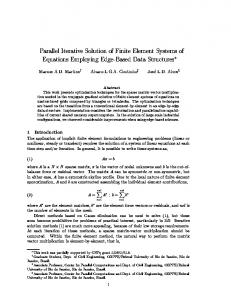
As we go along with examples it is fun to play around with plot commands and visualize what is computed. This section explains some useful visualization features. The plot(u) command launches a FEniCS component called Viper, which applies the VTK package to visualize finite element functions. Viper is not a full-fledged, easy-to-use front-end to VTK (like ParaView or VisIt), but rather a thin layer on top of VTK’s Python interface, allowing us to quickly visualize a DOLFIN function or mesh, or data in plain Numerical Python arrays, within a Python program. Viper is ideal for debugging, teaching, and initial scientific investigations. The visualization can be interactive, or you can steer and automate it through program statements. More advanced and professional visualizations are usually better done with advanced tools like MayaVi2, ParaView, or VisIt. We have made a program membrane1v.py for the membrane deflection problem in Section 1.1.5 and added various demonstrations of Viper capabilities. You are encouraged to play around with membrane1v.py and modify the code as you read about various features. The membrane1v.py program solves the two-dimensional Poisson equation for a scalar field w (the membrane deflection). The plot function can take additional arguments, such as a title of the plot, or a specification of a wireframe plot (elevated mesh) instead of a colored surface plot: Python code plot(mesh, title="Finite element mesh") plot(w, wireframe=True, title="solution")

1.1. FUNDAMENTALS

21

Figure 1.4: Plot of the deflection of a membrane.

1.00

Y

0.00

-1.00 0.00 -1.00

Z

0.00

1.00

X

The three mouse buttons can be used to rotate, translate, and zoom the surface. Pressing h in the plot window makes a printout of several key bindings that are available in such windows. For example, pressing m in the mesh plot window dumps the plot of the mesh to an Encapsulated PostScript (.eps) file, while pressing i saves the plot in PNG format. All file names are automatically generated as simulationX.eps, where X is a counter 0000, 0001, 0002, etc., being increased every time a new plot file in that format is generated (the extension of PNG files is .png instead of .eps). Pressing o adds a red outline of a bounding box around the domain. One can alternatively control the visualization from the program code directly. This is done through a Viper object returned from the plot command. Let us grab this object and use it to 1) tilt the camera −65 degrees in latitude direction, 2) add x and y axes, 3) change the default name of the plot files (generated by typing m and i in the plot window), 4) change the color scale, and 5) write the plot to a PNG and an EPS file. Here is the code: Python code viz_w = plot(w, wireframe=False, title="Scaled membrane deflection", rescale=False, axes=True, # include axes basename="deflection", # default plotfile name ) viz_w.elevate(-65) # tilt camera -65 degrees (latitude dir) viz_w.set_min_max(0, 0.5*max_w) # color scale viz_w.update(w) # bring settings above into action viz_w.write_png("deflection.png") viz_w.write_ps("deflection", format="eps")

The format argument in the latter line can also take the values "ps" for a standard PostScript file and "pdf" for a PDF file. Note the necessity of the viz_w.update(w) call – without it we will not see the effects of tilting the camera and changing the color scale. Figure 1.4 shows the resulting scalar surface.

CHAPTER 1. TUTORIAL

22 1.1.9

Combining Dirichlet and Neumann conditions

Let us make a slight extension of our two-dimensional Poisson problem from Section 1.1.1 and add a Neumann boundary condition. The domain is still the unit square, but now we set the Dirichlet condition u = u0 at the left and right sides, x = 0 and x = 1, while the Neumann condition

−

∂u =g ∂n

(1.27)

is applied to the remaining sides y = 0 and y = 1. The Neumann condition is also known as a natural boundary condition (in contrast to an essential boundary condition). Let Γ D and Γ N denote the parts of ∂Ω where the Dirichlet and Neumann conditions apply, respectively. The complete boundary-value problem can be written as

−∆u = f in Ω, u = u0 on Γ D , ∂u − = g on Γ N . ∂n

(1.28) (1.29) (1.30)

Again we choose u = 1 + x2 + 2y2 as the exact solution and adjust f , g, and u0 accordingly: f = −6, −4, g= 0,

(1.31) y=1 y=0

(1.32)

u0 = 1 + x2 + 2y2 .

(1.33)

For ease of programming we may introduce a g function defined over the whole of Ω such that g takes on the right values at y = 0 and y = 1. One possible extension is g( x, y) = −4y.

(1.34)

The first task is to derive the variational problem. This time we cannot omit the boundary term arising from the integration by parts, because v is only zero on Γ D . We have

−

Z

Ω

and since v = 0 on Γ D ,

−

(∆u)v dx =

Z

∂Ω

Z

Ω

∂u v ds = − ∂n

∇u · ∇v dx −

Z

Z

Z

ΓN

∂u v ds = ∂n

∂Ω

ΓN

∂u v ds, ∂n

(1.35)

gv ds,

(1.36)

by applying the boundary condition on Γ N . The resulting weak form reads Z

Ω

∇u · ∇v dx +

Z

ΓN

gv ds =

Z

Ω

f v dx.

(1.37)

Expressing (1.37) in the standard notation a(u, v) = L(v) is straightforward with a(u, v) = L(v) =

Z

ZΩ

Ω

∇u · ∇v dx, f v dx −

Z

ΓN

(1.38) gv ds.

(1.39)

1.1. FUNDAMENTALS

23

How does the Neumann condition impact the implementation? The code in the file Poisson2D_D2.py remains almost the same. Only two adjustments are necessary: 1. The function describing the boundary where Dirichlet conditions apply must be modified. 2. The new boundary term must be added to the expression in L. Step 1 can be coded as Python code def Dirichlet_boundary(x, on_boundary): if on_boundary: if x[0] == 0 or x[0] == 1: return True else: return False else: return False

A more compact implementation reads Python code def Dirichlet_boundary(x, on_boundary): return on_boundary and (x[0] == 0 or x[0] == 1)

As pointed out already in Section 1.1.3, testing for an exact match of real numbers is not good programming practice so we introduce a tolerance in the test: Python code def Dirichlet_boundary(x, on_boundary): tol = 1E-14 # tolerance for coordinate comparisons return on_boundary and \ (abs(x[0]) < tol or abs(x[0] - 1) < tol)

We may also split the boundary functions into two separate pieces, one for each part of the boundary: Python code tol = 1E-14 def Dirichlet_boundary0(x, on_boundary): return on_boundary and abs(x[0]) < tol def Dirichlet_boundary1(x, on_boundary): return on_boundary and abs(x[0] - 1) < tol bc0 = DirichletBC(V, Constant(0), Dirichlet_boundary0) bc1 = DirichletBC(V, Constant(1), Dirichlet_boundary1) bc = [bc0, bc1]

The second adjustment of our program concerns the definition of L, where we have to add a boundary integral and a definition of the g function to be integrated: Python code g = Expression("-4*x[1]") L = f*v*dx - g*v*ds

The ds variable implies a boundary integral, while dx implies an integral over the domain Ω. No more modifications are necessary. Running the resulting program, found in the file Poisson2D_DN1.py, shows a successful verification – u equals the exact solution at all the nodes, regardless of how many elements we use.

CHAPTER 1. TUTORIAL

24 1.1.10 Multiple Dirichlet conditions

The PDE problem from the previous section applies a function u0 ( x, y) for setting Dirichlet conditions at two parts of the boundary. Having a single function to set multiple Dirichlet conditions is seldom possible. The more general case is to have m functions for setting Dirichlet conditions on m parts of the boundary. The purpose of this section is to explain how such multiple conditions are treated in FEniCS programs. Let us return to the case from Section 1.1.9 and define two separate functions for the two Dirichlet conditions:

−∆u = −6 in Ω, u = u L on Γ0 , u = u R on Γ1 , ∂u = g on Γ N . − ∂n

(1.40) (1.41) (1.42) (1.43)

Here, Γ0 is the boundary x = 0, while Γ1 corresponds to the boundary x = 1. We have that u L = 1 + 2y2 , u R = 2 + 2y2 , and g = −4y. For the left boundary Γ0 we define the usual triple of a function for the boundary value, a function for defining the boundary of interest, and a DirichletBC object: Python code u_L = Expression("1 + 2*x[1]*x[1]") def left_boundary(x, on_nboundary): tol = 1E-14 # tolerance for coordinate comparisons return on_boundary and abs(x[0]) < tol Gamma_0 = DirichletBC(V, u_L, left_boundary)

For the boundary x = 1 we define a similar code: Python code u_R = Expression("2 + 2*x[1]*x[1]") def right_boundary(x, on_boundary): tol = 1E-14 # tolerance for coordinate comparisons return on_boundary and abs(x[0] - 1) < tol Gamma_1 = DirichletBC(V, u_R, right_boundary)

The various essential conditions are then collected in a list and passed onto our problem object of type VariationalProblem: Python code bc = [Gamma_0, Gamma_1] ... problem = VariationalProblem(a, L, bc)

If the u values are constant at a part of the boundary, we may use a simple Constant object instead of an Expression object. The file Poisson2D_DN2.py contains a complete program which demonstrates the constructions above. An extended example with multiple Neumann conditions would have been quite natural now, but this requires marking various parts of the boundary using the mesh function concept and is therefore left to Section 1.6.3.

1.1. FUNDAMENTALS

25

1.1.11 A linear algebra formulation Given a(u, v) = L(v), the discrete solution u is computed by inserting u = ∑ N j=1 U j φ j into a ( u, v ) and demanding a(u, v) = L(v) to be fulfilled for N test functions φˆ 1 , . . . , φˆ N . This implies N

∑ a(φj , φˆ i )Uj = L(φˆ i ),

i = 1, . . . , N,

(1.44)

j =1

which is nothing but a linear system, AU = b,

(1.45)

where the entries in A and b are given by Aij = a(φj , φˆ i ),

(1.46)

bi = L(φˆ i ).

The examples so far have constructed a VariationalProblem object and called its solve method to compute the solution u. The VariationalProblem object creates a linear system AU = b and calls an appropriate solution method for such systems. An alternative is dropping the use of a VariationalProblem object and instead asking FEniCS to create the matrix A and right-hand side b, and then solve for the solution vector U of the linear system. The relevant statements read Python code A = assemble(a) b = assemble(L) bc.apply(A, b) u = Function(V) solve(A, u.vector(), b)

The variables a and L are as before; that is, a refers to the bilinear form involving a TrialFunction object (say u) and a TestFunction object (v), and L involves a TestFunction object (v). From a and L, the assemble function can compute the matrix elements Ai,j and the vector elements bi . The matrix A and vector b are first assembled without incorporating essential (Dirichlet) boundary conditions. Thereafter, the bc.apply(A, b) call performs the necessary modifications to the linear system. The first three statements above can alternatively be carried out by4 Python code A, b = assemble_system(a, L, bc)

When we have multiple Dirichlet conditions stored in a list bc, as explained in Section 1.1.10, we must apply each condition in bc to the system: Python code # bc is a list of DirichletBC objects for condition in bc: condition.apply(A, b)

Alternatively, we can make the call Python code A, b = assemble_system(a, L, bc) 4 The

essential boundary conditions are now applied to the element matrices and vectors prior to assembly.

CHAPTER 1. TUTORIAL

26

The assemble_system function incorporates the boundary conditions in a symmetric way in the coefficient matrix. (For each degree of freedom that is known, the corresponding row and column is zeroed out and 1 is placed on the main diagonal, and the right-hand side b is modified by subtracting the column in A times the value of the degree of freedom, and then the corresponding entry in b is replaced by the known value of the degree of freedom.) With condition.apply(A, b), the matrix A is modified in an unsymmetric way. (The row is zeroed out and 1 is placed on the main diagonal, and the degree of freedom value is inserted in b.) Note that the solution u is, as before, a Function object. The degrees of freedom, U = A−1 b, are filled into u’s Vector object (u.vector()) by the solve function. The object A is of type Matrix, while b and u.vector() are of type Vector. We may convert the matrix and vector data to numpy arrays by calling the array() method as shown before. If you wonder how essential boundary conditions are incorporated in the linear system, you can print out A and b before and after the bc.apply(A, b) call: Python code if mesh.num_cells() < 16: print A.array() print b.array() bc.apply(A, b) if mesh.num_cells() < 16: print A.array() print b.array()

# print for small meshes only

With access to the elements in A as a numpy array we can easily do computations on this matrix, such as computing the eigenvalues (using the numpy.linalg.eig function). We can alternatively dump the matrix to file in MATLAB format and invoke MATLAB or Octave to perform computations: Python code mfile = File("A.m"); mfile tol and iter < maxiter: iter += 1 A, b = assemble_system(a, L, bc_du) solve(A, du.vector(), b) eps = numpy.linalg.norm(du.vector().array(), ord=numpy.Inf) print "Norm:", eps u.vector()[:] = uk.vector() + omega*du.vector() uk.assign(u)

There are other ways of implementing the update of the solution as well: Python code u.assign(uk) # u = uk u.vector().axpy(omega, du.vector()) # or u.vector()[:] += omega*du.vector()

The axpy(a, y) operation adds a scalar a times a Vector y to a Vector object. It is usually a fast operation calling up an optimized BLAS routine for the calculation. Mesh construction for a d-dimensional problem with arbitrary degree of the Lagrange elements can be done as explained in Section 1.1.14. The complete program appears in the file nlPoisson_algNewton.py. 1.2.3

A Newton method at the PDE level

Although Newton’s method in PDE problems is normally formulated at the linear algebra level; that is, as a solution method for systems of nonlinear algebraic equations, we can also formulate the method at the PDE level. This approach yields a linearization of the PDEs before they are discretized. FEniCS users will probably find this technique simpler to apply than the more standard method of Section 1.2.2. Given an approximation to the solution field, uk , we seek a perturbation δu so that uk+1 = uk + δu

(1.77)

fulfills the nonlinear PDE. However, the problem for δu is still nonlinear and nothing is gained. The idea is therefore to assume that δu is sufficiently small so that we can linearize the problem with

1.2. NONLINEAR PROBLEMS

39

respect to δu. Inserting uk+1 in the PDE, linearizing the q term as q(uk+1 ) = q(uk ) + q0 (uk )δu + O((δu)2 ) ≈ q(uk ) + q0 (uk )δu,

(1.78)

and dropping other nonlinear terms in δu, we get ∇ · q(uk )∇uk + ∇ · q(uk )∇δu + ∇ · q0 (uk )δu∇uk = 0.

We may collect the terms with the unknown δu on the left-hand side, ∇ · q(uk )∇δu + ∇ · q0 (uk )δu∇uk = −∇ · q(uk )∇uk ,

(1.79)

The weak form of this PDE is derived by multiplying by a test function v and integrating over Ω, integrating the second-order derivatives by parts: Z Ω

Z q(uk )∇δu · ∇v + q0 (uk )δu∇uk · ∇v dx = − q(uk )∇uk · ∇v dx. Ω

(1.80)

ˆ where The variational problem reads: find δu ∈ V such that a(δu, v) = L(v) for all v ∈ V, a(δu, v) =

Z Ω

L(v) = −

Z

q(uk )∇δu · ∇v + q0 (uk )δu∇uk · ∇v dx,

Ω

q(uk )∇uk · ∇v dx.

(1.81) (1.82)

ˆ being continuous or discrete, are as in the linear Poisson problem from The function spaces V and V, Section 1.1.2. We must provide some initial guess, e.g., the solution of the PDE with q(u) = 1. The corresponding weak form a0 (u0 , v) = L0 (v) has a0 (u, v) =

Z

Ω

∇u · ∇v dx,

L(v) = 0.

(1.83)

Thereafter, we enter a loop and solve a(δu, v) = L(v) for δu and compute a new approximation uk+1 = uk + δu. Note that δu is a correction, so if u0 satisfies the prescribed Dirichlet conditions on some part Γ D of the boundary, we must demand δu = 0 on Γ D . Looking at (1.81) and (1.82), we see that the variational form is the same as for the Newton method at the algebraic level in Section 1.2.2. Since Newton’s method at the algebraic level required some “backward” construction of the underlying weak forms, FEniCS users may prefer Newton’s method at the PDE level, which is more straightforward. There is seemingly no need for differentiations to derive a Jacobian matrix, but a mathematically equivalent derivation is done when nonlinear terms are linearized using the first two Taylor series terms and when products in the perturbation δu are neglected. The implementation is identical to the one in Section 1.2.2 and is found in the file nlPoisson_pdeNewton.py (for the fun of it we use a VariationalProblem object instead of assembling a matrix and vector and calling solve). The reader is encouraged to go through this code to be convinced that the present method actually ends up with the same program as needed for the Newton method at the linear algebra level in Section 1.2.2.

CHAPTER 1. TUTORIAL

40 1.2.4

Solving the nonlinear variational problem directly

DOLFIN has a built-in Newton solver and is able to automate the computation of nonlinear, stationary boundary-value problems. The automation is demonstrated next. A nonlinear variational problem (1.58) can be solved by Python code VariationalProblem(J, F, bc)

where F corresponds to the nonlinear form F (u; v) and J is a form for the derivative of F. The F form corresponding to (1.59) is straightforwardly defined (assuming q(u) is coded as a Python function): Python code v = TestFunction(V) u = Function(V) # the unknown F = inner(q(u)*grad(u), grad(v))*dx

Note here that u is a Function, not a TrialFunction. We could, alternatively, define F (u; v) directly in terms of a trial function for u and a test function for v, and then created the proper F by Python code u = v = Fuv u = F =

TrialFunction(V) TestFunction(V) = inner(q(u)*grad(u), grad(v))*dx Function(V) # previous guess action(Fuv, u)

The latter statement is equivalent to F (u = u0 ; v), where u0 is an existing finite element function representing the most recently computed approximation to the solution. The derivative J (J) of F (F) is formally the Gateaux derivative DF (uk ; δu, v) of F (u; v) at u = uk in the direction of δu. Technically, this Gateaux derivative is derived by computing d Fi (uk + eδu; v) e→0 de lim

(1.84)

The δu is now the trial function and uk is as usual the previous approximation to the solution u. We start with Z d ∇v · q(uk + eδu)∇(uk + eδu) dx (1.85) de Ω and obtain

which leads to

Z

Ω

h i ∇v · q0 (uk + eδu)δu∇(uk + eδu) + q(uk + eδu)∇δu dx, Z

Ω

(1.86)

h i ∇v · q0 (uk )δu∇(uk ) + q(uk )∇δu dx,

(1.87)

as e → 0. This last expression is the Gateaux derivative of F. We may use J or a(δu, v) for this derivative, the latter having the advantage that we easily recognize the expression as a bilinear form. However, in the forthcoming code examples J is used as variable name for the Jacobian. The specification of J goes as follows: Python code du = TrialFunction(V) J = inner(q(u)*grad(du), grad(v))*dx + \

1.3. TIME-DEPENDENT PROBLEMS

41

inner(Dq(u)*du*grad(u), grad(v))*dx

where u is a Function representing the most recent solution. The UFL language that we use to specify weak forms supports differentiation of forms. This means that when F is given as above, we can simply compute the Gateaux derivative by Python code J = derivative(F, u, du)

The differentiation is done symbolically so no numerical approximation formulas are involved. The derivative function is obviously very convenient in problems where differentiating F by hand implies lengthy calculations. The solution of the nonlinear problem is now a question of two statements: Python code problem = VariationalProblem(J, F, bc) u = problem.solve(u)

The u we feed to problem.solve is filled with the solution and returned, implying that the u on the lefthand side actually refers to the same u as provided on the right-hand side5 . The file nlPoisson_vp1.py contains the complete code, where J is calculated manually, while nlPoisson_vp2.py is a counterpart where J is computed by derivative(F, u, du). The latter file represents clearly the most automated way of solving the present nonlinear problem in FEniCS.

1.3

Time-dependent problems

The examples in Section 1.1 illustrate that solving linear, stationary PDE problems with the aid of FEniCS is easy and requires little programming. That is, FEniCS automates the spatial discretization by the finite element method. The solution of nonlinear problems, as we showed in Section 1.2, can also be automated (see Section 1.2.4), but many scientists will prefer to code the solution strategy of the nonlinear problem themselves and experiment with various combinations of strategies in difficult problems. Time-dependent problems are somewhat similar in this respect: we have to add a time discretization scheme, which is often quite simple, making it natural to explicitly code the details of the scheme so that the programmer has full control. We shall explain how easily this is accomplished through examples. 1.3.1

A diffusion problem and its discretization

Our time-dependent model problem for teaching purposes is naturally the simplest extension of the Poisson problem into the time domain; that is, the diffusion problem ∂u = ∆u + f in Ω, for t > 0, ∂t u = u0 on ∂Ω, for t > 0, u = I at t = 0.

(1.88) (1.89) (1.90)

5 Python has a convention that all input data to a function or class method are represented as arguments, while all output data are returned to the calling code. Data used as both input and output, as in this case, will then be arguments and returned. It is not necessary to have a variable on the left-hand side, as the function object is modified correctly anyway, but it is convention that we follow here.

CHAPTER 1. TUTORIAL

42

Here, u varies with space and time, e.g., u = u( x, y, t) if the spatial domain Ω is two-dimensional. The source function f and the boundary values u0 may also vary with space and time. The initial condition I is a function of space only. A straightforward approach to solving time-dependent PDEs by the finite element method is to first discretize the time derivative by a finite difference approximation, which yields a recursive set of stationary problems, and then turn each stationary problem into a variational formulation. Let superscript k denote a quantity at time tk , where k is an integer counting time levels. For example, uk means u at time level k. A finite difference discretization in time first consists in sampling the PDE at some time level, say k: ∂ k u = ∆uk + f k . (1.91) ∂t The time-derivative can be approximated by a finite difference. For simplicity and stability reasons we choose a simple backward difference: ∂ k u k − u k −1 u ≈ , ∂t dt

(1.92)

where dt is the time discretization parameter. Inserting (1.92) in (1.91) yields u k − u k −1 = ∆uk + f k . dt

(1.93)

This is our time-discrete version of the diffusion PDE (1.88). Reordering (1.93) so that uk appears on the left-hand side only, shows that (1.93) is a recursive set of spatial (stationary) problems for uk (assuming uk−1 is known from computations at the previous time level): u0 = I,

(1.94)

uk − dt∆uk = uk−1 + dt f k ,

k = 1, 2, . . .

(1.95)

Given I, we can solve for u0 , u1 , u2 , and so on. We use a finite element method to solve the equations (1.94) and (1.95). This requires turning the equations into weak forms. As usual, we multiply by a test function v ∈ Vˆ and integrate secondderivatives by parts. Introducing the symbol u for uk (which is natural in the program too), the resulting weak form can be conveniently written in the standard notation: a0 (u, v) = L0 (v) for (1.94) and a(u, v) = L(v) for (1.95), where a0 (u, v) = L0 ( v ) = a(u, v) = L(v) =

Z

ZΩ

ZΩ

uv dx,

(1.96)

Iv dx,

(1.97)

(uv + dt∇u · ∇v) dx, uk−1 + dt f k v dx.

(1.98)

ZΩ Ω

(1.99)

ˆ The continuous variational problem is to find u0 ∈ V such that a0 (u0 , v) = L0 (v) holds for all v ∈ V, k k ˆ and then find u ∈ V such that a(u , v) = L(v) for all v ∈ V, k = 1, 2, . . .. Approximate solutions in space are found by restricting the functional spaces V and Vˆ to finitedimensional spaces, exactly as we have done in the Poisson problems. We shall use the symbol u for the finite element approximation at time tk . In case we need to distinguish this space-time discrete


43

approximation from the exact solution of the continuous diffusion problem, we use ue for the latter. By uk−1 we mean, from now on, the finite element approximation of the solution at time tk−1 . Note that the forms a0 and L0 are identical to the forms met in Section 1.1.6, except that the test and trial functions are now scalar fields and not vector fields. Instead of solving (1.94) by a finite element method; that is, projecting I onto V via the problem a0 (u, v) = L0 (v), we could simply interpolate u0 0 from I. That is, if u0 = ∑ N j=1 U j φ j , we simply set U j = I ( x j , y j ), where ( x j , y j ) are the coordinates of node number j. We refer to these two strategies as computing the initial condition by either projecting I or interpolating I. Both operations are easy to compute through one statement, using either the project or interpolate function. 1.3.2

Implementation

Our program needs to perform the time stepping explicitly, but can rely on FEniCS to easily compute a0 , L0 , a, and L, and solve the linear systems for the unknowns. We realize that a does not depend on time, which means that its associated matrix also will be time independent. Therefore, it is wise to explicitly create matrices and vectors as in Section 1.1.11. The matrix A arising from a can be computed prior to the time stepping, so that we only need to compute the right-hand side b, corresponding to L, in each pass in the time loop. Let us express the solution procedure in algorithmic form, writing u for uk and uprev for the previous solution uk−1 : define Dirichlet boundary condition (u0 , Dirichlet boundary, etc.) if uprev is to be computed by projecting I: define a0 and L0 assemble matrix M from a0 and vector b from L0 solve MU = b and store U in uprev else: (interpolation) let uprev interpolate I define a and L assemble matrix A from a set some stopping time T t = dt while t 6 T assemble vector b from L apply essential boundary conditions solve AU = b for U and store in u t ← t + dt uprev ← u (be ready for next step) Before starting the coding, we shall construct a problem where it is easy to determine if the calculations are correct. The simple backward time difference is exact for linear functions, so we decide to have a linear variation in time. Combining a second-degree polynomial in space with a linear term in time, u = 1 + x2 + αy2 + βt, (1.100) yields a function whose computed values at the nodes may be exact, regardless of the size of the elements and dt, as long as the mesh is uniformly partitioned. Inserting (1.100) in the PDE problem (1.88), it follows that u0 must be given as (1.100) and that f ( x, y, t) = β − 2 − 2α and I ( x, y) = 1 + x2 + αy2 . A new programming issue is how to deal with functions that vary in space and time, such as the boundary condition u0 given by (1.100). Given a mesh and an associated function space V, we can specify the u0 function as

CHAPTER 1. TUTORIAL

44

Python code alpha = 3; beta = 1.2 u0 = Expression("1 + x[0]*x[0] + alpha*x[1]*x[1] + beta*t", {"alpha": alpha, "beta": beta}) u0.t = 0

This function expression has the components of x as independent variables, while alpha, beta, and t are parameters. The parameters can either be set through a dictionary at construction time, as demonstrated for alpha and beta, or anytime through attributes in the function object, as shown for the t parameter. The essential boundary conditions, along the whole boundary in this case, are set in the usual way, Python code def boundary(x, on_boundary): return on_boundary

# define the Dirichlet boundary

bc = DirichletBC(V, u0, boundary)

The initial condition can be computed by either projecting or interpolating I. The I ( x, y) function is available in the program through u0, as long as u0.t is zero. We can then do Python code u_prev = interpolate(u0, V) # or u_prev = project(u0, V)

Note that we could, as an equivalent alternative to using project, define a0 and L0 as we did in Section 1.1.6 and form a VariationalProblem object. To actually recover (1.100) to machine precision, it is important not to compute the discrete initial condition by projecting I, but by interpolating I so that the nodal values are exact at t = 0 (projection will imply approximative values at the nodes). The definition of a and L goes as follows: Python code dt = 0.3

# time step

u = TrialFunction(V) v = TestFunction(V) f = Constant(beta - 2 - 2*alpha) a = u*v*dx + dt*inner(grad(u), grad(v))*dx L = (u_prev + dt*f)*v*dx A = assemble(a)

# assemble only once, before the time stepping

Finally, we perform the time stepping in a loop: Python code u = Function(V) T = 2 t = dt

# the unknown at a new time level # total simulation time

while t 1. As N → ∞, the solve operation will dominate for α > 1, but for the values of N typically used on smaller computers, the assembly step may still represent a considerable part of the total work at each time level. Avoiding repeated assembly can therefore contribute to a significant speed-up of a finite element code in time-dependent problems. To see how repeated assembly can be avoided, we look at the L(v) form in (1.99), which in general varies with time through uk−1 , f k , and possibly also with dt if the time step is adjusted during the simulation. The technique for avoiding repeated assembly consists in expanding the finite element functions in sums over the basis functions φi , as explained in Section 1.1.11, to identify matrix-vector k −1 products that build up the complete system. We have uk−1 = ∑ N φj , and we can expand f k as j =1 U j k ˆ f k = ∑N j=1 F φ j . Inserting these expressions in L ( v ) and using v = φi result in j

Z Ω

uk−1 + dt f k v dx =

Z

Ω

N

=

∑

j =1

N

N

j =1

j =1

∑ Ujk−1 φj + dt ∑ Fjk φj

Z

Ω

φˆ i φj dx

Ujk−1

! N

+ dt ∑

j =1

φˆ i dx, Z

Ω

φˆ i φj dx

(1.101) Fjk .

CHAPTER 1. TUTORIAL

46 Introducing Mij =

R

Ω

φˆ i φj dx, we see that the last expression can be written N

∑

j =1

N

Mij Ujk−1 + dt ∑ Mij Fjk ,

(1.102)

j =1

which is nothing but two matrix-vector products, MU k−1 + dtMF k ,

(1.103)

k −1 T ) , U k−1 = (U1k−1 , . . . , UN

(1.104)

k T F k = ( F1k , . . . , FN ) .

(1.105)

if M is the matrix with entries Mij and

and We have immediate access to U k−1 in the program since that is the vector in the u_prev function. The F k vector can easily be computed by interpolating the prescribed f function (at each time level if f varies with time). Given M, U k−1 , and F k , the right-hand side b can be calculated as b = MU k−1 + dtMF k .

(1.106)

That is, no assembly is necessary to compute b. k The coefficient matrix A can also be split into two terms. We insert v = φˆ i and uk = ∑ N j=1 U j φ j in the expression (1.98) to get N

∑

j =1

Z

Ω

N Z k ˆ ˆ φi φj dx Uj + dt ∑ ∇φi · ∇φj dx Ujk , j =1

Ω

(1.107)

which can be written as a sum of matrix-vector products, MU k + dtKU k = ( M + dtK )U k ,

(1.108)

if we identify the matrix M with entries Mij as above and the matrix K with entries Kij =

Z

Ω

∇φˆ i · ∇φj dx.

(1.109)

The matrix M is often called the “mass matrix” while “stiffness matrix” is a common nickname for K. The associated bilinear forms for these matrices, as we need them for the assembly process in a FEniCS program, become aK (u, v) = a M (u, v) =

Z

ZΩ Ω

∇u · ∇v dx,

(1.110)

uv dx.

(1.111)

The linear system at each time level, written as AU k = b, can now be computed by first computing M and K, and then forming A = M + dtK at t = 0, while b is computed as b = MU k−1 + dtMF k at each time level. The following modifications are needed in the diffusion2D_D1.py program from the previous


47

section in order to implement the new strategy of avoiding assembly at each time level: 1. Define separate forms a M and aK 2. Assemble a M to M and aK to K 3. Compute A = M + dt K 4. Define f as an Expression 5. Interpolate the formula for f to a finite element function F k 6. Compute b = MU k−1 + dtMF k The relevant code segments become Python code # 1. a_K = inner(grad(u), grad(v))*dx a_M = u*v*dx # M K A

2. and 3. = assemble(a_M) = assemble(a_K) = M + dt*K

# 4. f = Expression("beta - 2 - 2*alpha", {"beta": beta, "alpha": alpha}) # 5. and 6. while t -0.5/4 && x[0] < 0.5/4 && x[1] > -1.0/2 && x[1] < -1.0/2 + 1.0/4 ? 1e-03 : 0.2

for D = 1 and W = D/2 (the string is one line, but broken into two here to fit the page width). It is very important to have a D that is float and not int, otherwise one gets integer divisions in the C++ expression and a completely wrong κ function. We are now ready to define the initial condition and the a and L forms of our problem: Python code T_prev = interpolate(Constant(T_R), V) rho = 1 c = 1 period = 2*pi/omega t_stop = 5*period dt = period/20 # 20 time steps per period theta = 1 T v f a L

= = = = =

TrialFunction(V) TestFunction(V) Constant(0) rho*c*T*v*dx + theta*dt*kappa*inner(grad(T), grad(v))*dx (rho*c*T_prev*v + dt*f*v (1-theta)*dt*kappa*inner(grad(T), grad(v)))*dx

1.4. CONTROLLING THE SOLUTION OF LINEAR SYSTEMS

51

A = assemble(a) b = None # variable used for memory savings in assemble calls

We could, alternatively, break a and L up in subexpressions and assemble a mass matrix and stiffness matrix, as exemplified in Section 1.3.3, to avoid assembly of b at every time level. This modification is straightforward and left as an exercise. The speed-up can be significant in 3D problems. The time loop is very similar to what we have displayed in Section 1.3.2: Python code T = Function(V) # unknown at the current time level t = dt while t 1, stretches the mesh toward ξ = 0 (x = a), while η = ξ 1/s makes a stretching toward ξ = 1 (x = b). Mapping the η ∈ [0, 1] coordinates back to [ a, b] gives new, stretched x coordinates, x¯ = a + (b − a) (( x − a) b − a)s toward x = a, or x¯ = a + (b − a)

x−a b−a

1/s

(1.122)

(1.123)

toward x = b One way of creating more complex geometries is to transform the vertex coordinates in a rectangular mesh according to some formula. Say we want to create a part of a hollow cylinder of Θ degrees, with inner radius a and outer radius b. A standard mapping from polar coordinates to Cartesian ¯ y¯ ) space such that coordinates can be used to generate the hollow cylinder. Given a rectangle in ( x, a 6 x¯ 6 b and 0 6 y¯ 6 1, the mapping xˆ = x¯ cos(Θy¯ ),

yˆ = x¯ sin(Θy¯ ),

(1.124)

¯ y¯ ) geometry and maps it to a point ( x, ˆ yˆ ) in a hollow cylinder. takes a point in the rectangular ( x, The corresponding Python code for first stretching the mesh and then mapping it onto a hollow cylinder looks as follows: Python code Theta = pi/2 a, b = 1, 5.0 nr = 10 # divisions in r direction nt = 20 # divisions in theta direction mesh = Rectangle(a, 0, b, 1, nr, nt, "crossed") # x y s

First make a denser mesh towards r=a = mesh.coordinates()[:,0] = mesh.coordinates()[:,1] = 1.3

def denser(x, y): return [a + (b-a)*((x-a)/(b-a))**s, y] x_bar, y_bar = denser(x, y) xy_bar_coor = numpy.array([x_bar, y_bar]).transpose() mesh.coordinates()[:] = xy_bar_coor plot(mesh, title="stretched mesh")

1.6. HANDLING DOMAINS WITH DIFFERENT MATERIALS

57

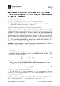
Figure 1.8: A hollow cylinder generated by mapping a rectangular mesh, stretched toward the left side.

def cylinder(r, s): return [r*numpy.cos(Theta*s), r*numpy.sin(Theta*s)] x_hat, y_hat = cylinder(x_bar, y_bar) xy_hat_coor = numpy.array([x_hat, y_hat]).transpose() mesh.coordinates()[:] = xy_hat_coor plot(mesh, title="hollow cylinder") interactive()

The result of calling denser and cylinder above is a list of two vectors, with the x and y coordinates, respectively. Turning this list into a numpy array object results in a 2 × M array, M being the number of vertices in the mesh. However, mesh.coordinates() is by a convention an M × 2 array so we need to take the transpose. The resulting mesh is displayed in Figure 1.8. Setting boundary conditions in meshes created from mappings like the one illustrated above is most conveniently done by using a mesh function to mark parts of the boundary. The marking is easiest to perform before the mesh is mapped since one can then conceptually work with the sides in a pure rectangle.

1.6

Handling domains with different materials

Solving PDEs in domains made up of different materials is a frequently encountered task. In FEniCS, these kind of problems are handled by defining subdomains inside the domain. The subdomains may represent the various materials. We can thereafter define material properties through functions, known in FEniCS as mesh functions, that are piecewise constant in each subdomain. A simple example with two materials (subdomains) in 2D will demonstrate the basic steps in the process. 1.6.1

Working with two subdomains

Suppose we want to solve

∇ · [k( x, y)∇u( x, y)] = 0,

(1.125)

in a domain Ω consisting of two subdomains where k takes on a different value in each subdomain. For simplicity, yet without loss of generality, we choose for the current implementation the domain

CHAPTER 1. TUTORIAL

58 y

Figure 1.9: Sketch of a Poisson problem with a variable coefficient that is constant in each of the two subdomains Ω0 and Ω1 .

6 u=1

Ω1 ∂u ∂n

∂u ∂n

=0

=0

Ω0 x

u=0

Ω = [0, 1] × [0, 1] and divide it into two equal subdomains, as depicted in Figure 1.9, Ω0 = [0, 1] × [0, 1/2],

Ω1 = [0, 1] × (1/2, 1].

(1.126)

We define k( x, y) = k0 in Ω0 and k( x, y) = k1 in Ω1 , where k0 > 0 and k1 > 0 are given constants. As boundary conditions, we choose u = 0 at y = 0, u = 1 at y = 1, and ∂u/∂n = 0 at x = 0 and x = 1. One can show that the exact solution is now given by u( x, y) =

(

2yk1 k0 +k1 , (2y−1)k0 +k1 , k0 +k1

y 6 1/2 y > 1/2

(1.127)

As long as the element boundaries coincide with the internal boundary y = 1/2, this piecewise linear solution should be exactly recovered by Lagrange elements of any degree. We use this property to verify the implementation. Physically, the present problem may correspond to heat conduction, where the heat conduction in Ω1 is ten times more efficient than in Ω0 . An alternative interpretation is flow in porous media with two geological layers, where the layers’ ability to transport the fluid differs by a factor of 10. 1.6.2

Implementation

The new functionality in this subsection regards how to define the subdomains Ω0 and Ω1 . For this purpose we need to use subclasses of class SubDomain, not only plain functions as we have used so far for specifying boundaries. Consider the boundary function Python code def boundary(x, on_boundary): tol = 1E-14 return on_boundary and abs(x[0]) < tol

for defining the boundary x = 0. Instead of using such a stand-alone function, we can create an instance6 of a subclass of SubDomain, which implements the inside method as an alternative to the 6 The

term instance means a Python object of a particular type (such as SubDomain, Function, FunctionSpace, etc.). Many use instance and object as interchangeable terms. In other computer programming languages one may also use the term variable for


59

boundary function:

Python code class Boundary(SubDomain): def inside(x, on_boundary): tol = 1E-14 return on_boundary and abs(x[0]) < tol boundary = Boundary() bc = DirichletBC(V, Constant(0), boundary)

A subclass of SubDomain with an inside method offers functionality for marking parts of the domain or the boundary. Now we need to define one class for the subdomain Ω0 where y 6 1/2 and another for the subdomain Ω1 where y > 1/2: Python code class Omega0(SubDomain): def inside(self, x, on_boundary): return True if x[1] = 0.5 else False

Notice the use of = in both tests. For a cell to belong to, e.g., Ω1 , the inside method must return True for all the vertices x of the cell. So to make the cells at the internal boundary y = 1/2 belong to Ω1 , we need the test x[1] >= 0.5. The next task is to use a MeshFunction to mark all cells in Ω0 with the subdomain number 0 and all cells in Ω1 with the subdomain number 1. Our convention is to number subdomains as 0, 1, 2, . . .. A MeshFunction is a discrete function that can be evaluated at a set of so-called mesh entities. Examples on mesh entities are cells, facets, and vertices. A MeshFunction over cells is suitable to represent subdomains (materials), while a MeshFunction over facets is used to represent pieces of external or internal boundaries. Mesh functions over vertices can be used to describe continuous fields. Since we need to define subdomains of Ω in the present example, we must make use of a MeshFunction over cells. The MeshFunction constructor is fed with three arguments: 1) the type of value: "int" for integers, "uint" for positive (unsigned) integers, "double" for real numbers, and "bool" for logical values; 2) a Mesh object, and 3) the topological dimension of the mesh entity in question: cells have topological dimension equal to the number of space dimensions in the PDE problem, and facets have one dimension lower. Alternatively, the constructor can take just a filename and initialize the MeshFunction from data in a file. We start with creating a MeshFunction whose values are non-negative integers ("uint") for numbering the subdomains. The mesh entities of interest are the cells, which have dimension 2 in a two-dimensional problem (1 in 1D, 3 in 3D). The appropriate code for defining the MeshFunction for two subdomains then reads Python code subdomains = MeshFunction("uint", mesh, 2) # Mark subdomains with numbers 0 and 1 subdomain0 = Omega0() subdomain0.mark(subdomains, 0) subdomain1 = Omega1() subdomain1.mark(subdomains, 1)

the same thing. We mostly use the well-known term object in this text.

CHAPTER 1. TUTORIAL

60

Calling subdomains.values() returns a numpy array of the subdomain values. That is, subdomain.values()[i] is the subdomain value of cell number i. This array is used to look up the subdomain or material number of a specific element. We need a function k that is constant in each subdomain Ω0 and Ω1 . Since we want k to be a finite element function, it is natural to choose a space of functions that are constant over each element. The family of discontinuous Galerkin methods, in FEniCS denoted by "DG", is suitable for this purpose. Since we want functions that are piecewise constant, the value of the degree parameter is zero: Python code V0 = FunctionSpace(mesh, "DG", 0) k = Function(V0)

To fill k with the right values in each element, we loop over all cells (the indices in subdomain.values()), extract the corresponding subdomain number of a cell, and assign the corresponding k value to the k.vector() array: Python code k_values = [1.5, 50] # values of k in the two subdomains for cell_no in range(len(subdomains.values())): subdomain_no = subdomains.values()[cell_no] k.vector()[cell_no] = k_values[subdomain_no]

Long loops in Python are known to be slow, so for large meshes it is preferable to avoid such loops and instead use vectorized code. Normally this implies that the loop must be replaced by calls to functions from the numpy library that operate on complete arrays (in efficient C code). The functionality we want in the present case is to compute an array of the same size as subdomain.values(), but where the value i of an entry in subdomain.values() is replaced by k_values[i]. Such an operation is carried out by the numpy function choose: Python code help = numpy.asarray(subdomains.values(), dtype=numpy.int32) k.vector()[:] = numpy.choose(help, k_values)

The help array is required since choose cannot work with subdomain.values() because this array has elements of type uint32. We must therefore transform this array to an array help with standard int32 integers. Having the k function ready for finite element computations, we can proceed in the normal manner with defining essential boundary conditions, as in Section 1.1.10, and the a(u, v) and L(v) forms, as in Section 1.1.12. All the details can be found in the file Poisson2D_2mat.py. 1.6.3

Multiple Neumann, Robin, and Dirichlet conditions

Let us go back to the model problem from Section 1.1.10 where we had both Dirichlet and Neumann conditions. The term v*g*ds in the expression for L implies a boundary integral over the complete boundary, or in FEniCS terms, an integral over all exterior cell facets. However, the contributions from the parts of the boundary where we have Dirichlet conditions are erased when the linear system is modified by the Dirichlet conditions. We would like, from an efficiency point of view, to integrate v*g*ds only over the parts of the boundary where we actually have Neumann conditions. And more importantly, in other problems one may have different Neumann conditions or other conditions like the Robin type condition. With the mesh function concept we can mark different parts of the boundary and integrate over specific parts. The same concept can also be used to treat multiple Dirichlet conditions. The forthcoming text illustrates how this is done.


61

Essentially, we still stick to the model problem from Section 1.1.10, but replace the Neumann condition at y = 0 by a Robin condition7 :

−

∂u = p ( u − q ), ∂n

(1.128)

where p and q are specified functions. Since we have prescribed a simple solution in our model problem, u = 1 + x2 + 2y2 , we adjust p and q such that the condition holds at y = 0. This implies that q = 1 + x2 + 2y2 and p can be arbitrary (the normal derivative at y = 0: ∂u/∂n = −∂u/∂y = −4y = 0). Now we have four parts of the boundary: Γ N which corresponds to the upper side y = 1, Γ R which corresponds to the lower part y = 0, Γ0 which corresponds to the left part x = 0, and Γ1 which corresponds to the right part x = 1. The complete boundary-value problem reads

−∆u = −6 in Ω, u = u L on Γ0 , u = u R on Γ1 , ∂u − = p(u − q) on Γ R , ∂n ∂u − = g on Γ N . ∂n

(1.129) (1.130) (1.131) (1.132) (1.133)

The involved prescribed functions are u L = 1 + 2y2 , u R = 2 + 2y2 , q = 1 + x2 + 2y2 , p is arbitrary, and g = −4y. R Integration by parts of − Ω v∆u dx becomes as usual

−

Z

Ω

v∆u dx =

Z

Ω

∇u · ∇v dx −

Z

∂Ω

∂u v ds. ∂n

(1.134)

The boundary integral vanishes on Γ0 ∪ Γ1 , and we split the parts over Γ N and Γ R since we have different conditions at those parts:

−

Z

v ∂Ω

∂u ds = − ∂n

Z

ΓN

v

∂u ds − ∂n

Z

ΓR

v

∂u ds = ∂n

Z

ΓN

vg ds +

Z

ΓR

vp(u − q) ds.

(1.135)

The weak form then becomes Z

Ω

∇u · ∇v dx +

Z

ΓN

gv ds +

Z

ΓR

p(u − q)v ds =

Z

Ω

f v dx,

(1.136)

We want to write this weak form in the standard notation a(u, v) = L(v), which requires that we identify all integrals with both u and v, and collect these in a(u, v), while the remaining integrals with v and not u go into L(v). The integral from the Robin condition must of this reason be split in two parts: Z Z Z ΓR

7 The

p(u − q)v ds =

ΓR

puv ds −

ΓR

pqv ds.

(1.137)

Robin condition is most often used to model heat transfer to the surroundings and arise naturally from Newton’s cooling law.

CHAPTER 1. TUTORIAL

62 We then have a(u, v) = L(v) =

Z

Z

Ω

∇u · ∇v dx +

Ω

f v dx −

Z

ΓN

Z

ΓR

puv ds,

(1.138)

Z

(1.139)

gv ds +

ΓR

pqv ds.

A natural starting point for implementation is the Poisson2D_DN2.py program, which we now copy to Poisson2D_DNR.py. The new aspects are 1. definition of a mesh function over the boundary, 2. marking each side as a subdomain, using the mesh function, 3. splitting a boundary integral into parts. Task 1 makes use of the MeshFunction object, but contrary to Section 1.6.2, this is not a function over cells, but a function over cell facets. The topological dimension of cell facets is one lower than the cell interiors, so in a two-dimensional problem the dimension becomes 1. In general, the facet dimension is given as mesh.topology().dim()-1, which we use in the code for ease of direct reuse in other problems. The construction of a MeshFunction object to mark boundary parts now reads Python code boundary_parts = \ MeshFunction("uint", mesh, mesh.topology().dim()-1)

As in Section 1.6.2 we use a subclass of SubDomain to identify the various parts of the mesh function. Problems with domains of more complicated geometries may set the mesh function for marking boundaries as part of the mesh generation. In our case, the y = 0 boundary can be marked by Python code class LowerRobinBoundary(SubDomain): def inside(self, x, on_boundary): tol = 1E-14 # tolerance for coordinate comparisons return on_boundary and abs(x[1]) < tol Gamma_R = LowerRobinBoundary() Gamma_R.mark(boundary_parts, 0)

The code for the y = 1 boundary is similar and is seen in Poisson2D_DNR.py. The Dirichlet boundaries are marked similarly, using subdomain number 2 for Γ0 and 3 for Γ1 : Python code class LeftBoundary(SubDomain): def inside(self, x, on_boundary): tol = 1E-14 # tolerance for coordinate comparisons return on_boundary and abs(x[0]) < tol Gamma_0 = LeftBoundary() Gamma_0.mark(boundary_parts, 2) class RightBoundary(SubDomain): def inside(self, x, on_boundary): tol = 1E-14 # tolerance for coordinate comparisons return on_boundary and abs(x[0] - 1) < tol Gamma_1 = RightBoundary() Gamma_1.mark(boundary_parts, 3)

1.7. MORE EXAMPLES

63

Specifying the DirichletBC objects may now make use of the mesh function (instead of a SubDomain subclass object) and an indicator for which subdomain each condition should be applied to: Python code u_L = Expression("1 + 2*x[1]*x[1]") u_R = Expression("2 + 2*x[1]*x[1]") bc = [DirichletBC(V, u_L, boundary_parts, 2), DirichletBC(V, u_R, boundary_parts, 3)]

Some functions need to be defined before we can go on with the a and L of the variational problem: Python code g q p u v f

= = = = = =

Expression("-4*x[1]") Expression("1 + x[0]*x[0] + 2*x[1]*x[1]") Constant(100) # arbitrary function can go here TrialFunction(V) TestFunction(V) Constant(-6.0)

The new aspect of the variational problem is the two distinct boundary integrals. Having a mesh function over exterior cell facets (our boundary_parts object), where subdomains (boundary parts) are numbered as 0, 1, 2, . . ., the special symbol ds(0) implies integration over subdomain (part) 0, ds(1) denotes integration over subdomain (part) 1, and so on. The idea of multiple ds-type objects generalizes to volume integrals too: dx(0), dx(1), etc., are used to integrate over subdomain 0, 1, etc., inside Ω. The variational problem can be defined as Python code a = inner(grad(u), grad(v))*dx + p*u*v*ds(0) L = f*v*dx - g*v*ds(1) + p*q*v*ds(0)

For the ds(0) and ds(1) symbols to work we must obviously connect them (or a and L) to the mesh function marking parts of the boundary. This is done by a certain keyword argument to the assemble function: Python code A = assemble(a, exterior_facet_domains=boundary_parts) b = assemble(L, exterior_facet_domains=boundary_parts)

Then essential boundary conditions are enforced, and the system can be solved in the usual way: Python code for condition in bc: condition.apply(A, b) u = Function(V) solve(A, u.vector(), b)

At the time of this writing, it is not possible to perform integrals over different parts of the domain or boundary using the assemble_system function or the VariationalProblem object.

1.7

More examples

Many more topics could be treated in a FEniCS tutorial, e.g., how to solve systems of PDEs, how to work with mixed finite element methods, how to create more complicated meshes and mark boundaries, and how to create more advanced visualizations. However, to limit the size of this tutorial, the examples end here. There are, fortunately, a rich set of FEniCS demos. The FEniCS documentation

CHAPTER 1. TUTORIAL

64

explains a collection of PDE solvers in detail: the Poisson equation, the mixed formulation for the Poission equation, the Biharmonic equation, the equations of hyperelasticity, the Cahn-Hilliard equation, and the incompressible Navier-Stokes equations. Both Python and C++ versions of these solvers are explained. An eigenvalue solver is also documented. In the dolfin/demo directory of the DOLFIN source code tree you can find programs for these and many other examples, including the advection-diffusion equation, the equations of elastodynamics, a reaction-diffusion equation, various finite element methods for the Stokes problem, discontinuous Galerkin methods for the Poisson and advection-diffusion equations, and an eigenvalue problem arising from electromagnetic waveguide problem with Nédélec elements. There are also numerous demos on how to apply various functionality in FEniCS, e.g., mesh refinement and error control, moving meshes (for ALE methods), computing functionals over subsets of the mesh (such as lift and drag on bodies in flow), and creating separate subdomain meshes from a parent mesh. The project cbc.solve (https://launchpad.net/cbc.solve) offers more complete PDE solvers for the Navier-Stokes equations (Chapter 24), the equations of hyperelasticity (Chapter 29), fluid-structure interaction (Chapter 24), viscous mantle flow (Chapter 33), and the bidomain model of electrophysiology. Another project, cbc.rans (https://launchpad.net/cbc.rans), offers an environment for very flexible and easy implementation of systems of nonlinear PDEs in general, and a collection of NavierStokes solvers and turbulence models in particular Mortensen et al. [2011b,a]. For example, cbc.rans contains an elliptic relaxation model for turbulent flow involving 18 nonlinear PDEs. FEniCS proved to be an ideal environment for implementing such complicated PDE models.

1.8

Miscellaneous topics

1.8.1

Glossary

Below we explain some key terms used in this tutorial. FEniCS: name of a software suite composed of many individual software components (see fenicsproject.org). Some components are DOLFIN and Viper, explicitly referred to in this tutorial. Others are FFC and FIAT, heavily used by the programs appearing in this tutorial, but never explicitly used from the programs. DOLFIN: a FEniCS component, more precisely a C++ library, with a Python interface, for performing important actions in finite element programs. DOLFIN makes use of many other FEniCS components and many external software packages. Viper: a FEniCS component for quick visualization of finite element meshes and solutions. UFL: a FEniCS component implementing the unified form language for specifying finite element forms in FEniCS programs. The definition of the forms, typically called a and L in this tutorial, must have legal UFL syntax. The same applies to the definition of functionals (see Section 1.1.7). Class (Python): a programming construction for creating objects containing a set of variables and functions. Most types of FEniCS objects are defined through the class concept. Instance (Python): an object of a particular type, where the type is implemented as a class. For instance, mesh = UnitInterval(10) creates an instance of class UnitInterval, which is reached by the name mesh. (Class UnitInterval is actually just an interface to a corresponding C++ class in the DOLFIN C++ library.) Class method (Python): a function in a class, reached by dot notation: instance_name.method_name self parameter (Python): required first parameter in class methods, representing a particular

1.8. MISCELLANEOUS TOPICS

65

object of the class. Used in method definitions, but never in calls to a method. For example, if method(self, x) is the definition of method in a class Y, method is called as y.method(x), where y is an instance of class X. In a call like y.method(x), method is invoked with self=y. Class attribute (Python): a variable in a class, reached by dot notation: instance_name.attribute_name 1.8.2

Overview of objects and functions

Most classes in FEniCS have an explanation of the purpose and usage that can be seen by using the general documentation command pydoc for Python objects. You can type Output pydoc dolfin.X

to look up documentation of a Python class X from the DOLFIN library (X can be UnitSquare, Function, Viper, etc.). Below is an overview of the most important classes and functions in FEniCS programs, in the order they typically appear within programs. UnitSquare(nx, ny): generate mesh over the unit square [0, 1] × [0, 1] using nx divisions in x direction and ny divisions in y direction. Each of the nx*ny squares are divided into two cells of triangular shape. UnitInterval, UnitCube, UnitCircle, UnitSphere, Interval, Rectangle, and Box: generate mesh over domains of simple geometric shape, see Section 1.5. FunctionSpace(mesh, element_type, degree): a function space defined over a mesh, with a given element type (e.g., "Lagrange" or "DG"), with basis functions as polynomials of a specified

degree. Expression(formula): a scalar- or vector-valued function, given as a mathematical expression formula (string) written in C++ syntax. Function(V): a scalar- or vector-valued finite element field in the function space V. If V is a FunctionSpace object, Function(V) becomes a scalar field, and with V as a VectorFunctionSpace object, Function(V) becomes a vector field. SubDomain: class for defining a subdomain, either a part of the boundary, an internal boundary, or a part of the domain. The programmer must subclass SubDomain and implement the inside(self, x, on_boundary) function (see Section 1.1.3) for telling whether a point x is inside the subdomain or not. Mesh: class for representing a finite element mesh, consisting of cells, vertices, and optionally faces,

edges, and facets. MeshFunction: tool for marking parts of the domain or the boundary. Used for variable coefficients (“material properties”, see Section 1.6.1) or for boundary conditions (see Section 1.6.3). DirichletBC(V, value, where): specification of Dirichlet (essential) boundary conditions via a function space V, a function value(x) for computing the value of the condition at a point x, and a specification where of the boundary, either as a SubDomain subclass instance, a plain function, or as a MeshFunction instance. In the latter case, a 4th argument is provided to describe which subdomain number that describes the relevant boundary. TrialFunction(V): define a trial function on a space V to be used in a variational form to represent the unknown in a finite element problem. TestFunction(V): define a test function on a space V to be used in a variational form.

CHAPTER 1. TUTORIAL

66

assemble(X): assemble a matrix, a right-hand side, or a functional, given a from X written with

UFL syntax. assemble_system(a, L, bc): assemble the matrix and the right-hand side from a bilinear (a) and linear (L) form written with UFL syntax. The bc parameter holds one or more DirichletBC objects. VariationalProblem(a, L, bc): define and solve a variational problem, given a bilinear (a) and linear (L) form, written with UFL syntax, and one or more DirichletBC objects stored in bc. solve(A, U, b): solve a linear system with A as coefficient matrix (Matrix object), U as unknown (Vector object), and b as right-hand side (Vector object). Usually, U is replaced by u.vector(), where u is a Function object representing the unknown finite element function of the problem, while A and b are computed by calls to assemble or assemble_system. plot(q): quick visualization of a mesh, function, or mesh function q, using the Viper component

in FEniCS. interpolate(func, V): interpolate a formula or finite element function func onto the function

space V. project(func, V): project a formula or finite element function func onto the function space V.

1.8.3

Installing FEniCS

The FEniCS software components are available for Linux, Windows and Mac OS X platforms. Detailed information on how to get FEniCS running on such machines are available at the fenicsproject.org website. Here are just some quick descriptions and recommendations by the author. To make the installation of FEniCS as painless and reliable as possible, the reader is strongly recommended to use Ubuntu Linux8 . Any standard PC can easily be equipped with Ubuntu Linux, which may live side by side with either Windows or Mac OS X or another Linux installation. Basically, you download Ubuntu from http://www.ubuntu.com/getubuntu/download, burn the file on a CD, reboot the machine with the CD, and answer some usually straightforward questions (if necessary). The graphical user interface (GUI) of Ubuntu is quite similar to both Windows 7 and Mac OS X, but to be efficient when doing science with FEniCS this author recommends to run programs in a terminal window and write them in a text editor like Emacs or Vim. You can employ integrated development environment such as Eclipse, but intensive FEniCS developers and users tend to find terminal windows and plain text editors more user friendly. Instead of making it possible to boot your machine with the Linux Ubuntu operating system, you can run Ubuntu in a separate window in your existing operation system. On Mac, you can use the VirtualBox software available from http://www.virtualbox.org to run Ubuntu. On Windows, Wubi makes a tool that automatically installs Ubuntu on the machine. Just give a user name and password for the Ubuntu installation, and Wubi performs the rest. You can also use VirtualBox on Windows machines. Once the Ubuntu window is up and running, FEniCS is painlessly installed by Bash code sudo apt-get install fenics

Sometimes the FEniCS software in a standard Ubuntu installation lacks some recent features and bug fixes. Visiting fenicsproject.org and copying just five Unix commands is all you have to do to 8 Even

though Mac users now can get FEniCS by a one-click install, I recommend using Ubuntu on Mac, unless you have high Unix competence and much experience with compiling and linking C++ libraries on Mac OS X.

1.8. MISCELLANEOUS TOPICS

67

install a newer version of the software. 1.8.4

Books on the finite element method

There are a large number of books on the finite element method. The books typically fall in either of two categories: the abstract mathematical version of the method and the engineering “structural analysis” formulation. FEniCS builds heavily on concepts in the abstract mathematical exposition. An easy-to-read book, which provides a good general background for using FEniCS, is Gockenbach [2006]. The book Donea and Huerta [2003] has a similar style, but aims at readers with interest in fluid flow problems. Hughes [1987] is also highly recommended, especially for those interested in solid mechanics and heat transfer applications. Readers with background in the engineering “structural analysis” version of the finite element method may find Bickford [1994] as an attractive bridge over to the abstract mathematical formulation that FEniCS builds upon. Those who have a weak background in differential equations in general should consult a more fundamental book, and Eriksson et al. [1996] is a very good choice. On the other hand, FEniCS users with a strong background in mathematics and interest in the mathematical properties of the finite element method, will appreciate the texts Brenner and Scott [2008], Braess [2007], Ern and Guermond [2004], Quarteroni and Valli [2008], or Ciarlet [2002]. 1.8.5

Books on Python

Two very popular introductory books on Python are “Learning Python” [Lutz, 2007] and “Practical Python” [Hetland, 2002]. More advanced and comprehensive books include “Programming Python” [Lutz, 2006], and “Python Cookbook” [Martelli and Ascher, 2005] and “Python in a Nutshell” [Martelli, 2006]. The web page http://wiki.python.org/moin/PythonBooks lists numerous additional books. Very few texts teach Python in a mathematical and numerical context, but the references Langtangen [2008, 2011], Kiusalaas [2009] are exceptions. 1.8.6

User-defined functions

When defining a function in terms of a mathematical expression inside a string formula, e.g., Python code myfunc = Expression("sin(x[0])*cos(x[1])")

the expression contained in the first argument will be turned into a C++ function and compiled to gain efficiency. Therefore, the syntax used in the expression must be valid C++ syntax. Most Python syntax for mathematical expressions are also valid C++ syntax, but power expressions make an exception: p**a must be written as pow(p,a) in C++ (this is also an alternative Python syntax). The following mathematical functions can be used directly in C++ expressions when defining Expression objects: cos, sin, tan, acos, asin, atan, atan2, cosh, sinh, tanh, exp, frexp, ldexp, log, log10, modf, pow, sqrt, ceil, fabs, floor, and fmod. Moreover, the number π is available as the symbol pi. All the listed functions are taken from the cmath C++ header file, and one may hence consult documentation of cmath for more information on the various functions. Acknowledgments. The author is very thankful to Johan Hake, Anders Logg, Kent-Andre Mardal, and Kristian Valen-Sendstad for promptly answering all my questions about FEniCS functionality and for implementing all my requests. I will in particular thank Professor Douglas Arnold for very valuable feedback on the text. Øystein Sørensen pointed out a lot of typos and contributed with many helpful comments. Many errors and typos were also reported by Mauricio Angeles, Ida Drøsdal, and

68

CHAPTER 1. TUTORIAL

Hans Ekkehard Plesser. Ekkehard Ellmann as well as two anonymous reviewers provided a series of suggestions and improvements.

Part I

Methodology

69

2

The finite element method

By Robert C. Kirby and Anders Logg

The finite element method has emerged as a universal method for the solution of differential equations. Much of the success of the finite element method can be attributed to its generality and elegance, allowing a wide range of differential equations from all areas of science to be analyzed and solved within a common framework. Another contributing factor to the success of the finite element method is the flexibility of formulation, allowing the properties of the discretization to be controlled by the choice of approximating finite element spaces. In this chapter, we review the finite element method and summarize some basic concepts and notation used throughout this book. In the coming chapters, we discuss these concepts in more detail, with a particular focus on the implementation and automation of the finite element method as part of the FEniCS project.

2.1

A simple model problem

In 1813, Siméon Denis Poisson published in Bulletin de la société philomatique his famous equation as a correction of an equation published earlier by Pierre-Simon Laplace. Poisson’s equation is a second-order partial differential equation stating that the negative Laplacian −∆u of some unknown field u = u( x ) is equal to a given function f = f ( x ) on a domain Ω ⊂ Rd , possibly amended by a set of boundary conditions for the solution u on the boundary ∂Ω of Ω:

−∆u = f u = u0 −∂n u = g

in Ω, on ΓD ⊂ ∂Ω, on ΓN ⊂ ∂Ω.

(2.1)

The Dirichlet boundary condition u = u0 signifies a prescribed value for the unknown u on a subset ΓD of the boundary, and the Neumann boundary condition −∂n u = g signifies a prescribed value for the (negative) normal derivative of u on the remaining boundary ΓN = ∂Ω \ ΓD . Poisson’s equation is a simple model for gravity, electromagnetism, heat transfer, fluid flow, and many other physical processes. It also appears as the basic building block in a large number of more complex physical models, including the Navier–Stokes equations which we return to in Chapters 21, 20, 21, 22, 23, 24, 25, 26, 27, and 28. To derive Poisson’s equation (2.1), we may consider a model for the temperature u in a body occupying a domain Ω subject to a heat source f . Letting σ = σ ( x ) denote heat flux, it follows by conservation of energy that the outflow of energy over the boundary ∂ω of any test volume ω ⊂ Ω must be balanced by the energy emitted by the heat source f : Z

∂ω

σ · n ds = 71

Z

f dx. ω

(2.2)

CHAPTER 2. THE FINITE ELEMENT METHOD

72

Figure 2.1: Poisson’s equation is a simple consequence of balance of energy in an arbitrary test volume ω ⊂ Ω.

n

σ = −κ ∇ u

Ω

ω

Integrating by parts, we find that

Z

ω

∇ · σ dx =

Z

f dx.

(2.3)

ω

Since (2.3) holds for all test volumes ω ⊂ Ω, it follows that ∇ · σ = f throughout Ω (with suitable regularity assumptions on σ and f ). If we now make the assumption that the heat flux σ is proportional to the negative gradient of the temperature u (Fourier’s law), σ = −κ ∇u,

(2.4)

we arrive at the following system of equations:

∇·σ = f σ + ∇u = 0

in Ω, in Ω,

(2.5)

where we have assumed that the heat conductivity is κ = 1. Replacing σ in the first of these equations by −∇u, we arrive at Poisson’s equation (2.1). Note that one may as well arrive at the system of first-order equations (2.5) by introducing σ = −∇u as an auxiliary variable in the second-order equation (2.1). We also note that the Dirichlet and Neumann boundary conditions in (2.1) correspond to prescribed values for the temperature and heat flux respectively.

2.2

Finite element discretization

2.2.1

Discretizing Poisson’s equation

To discretize Poisson’s equation (2.1) by the finite element method, we first multiply by a test function v and integrate by parts to obtain Z

Ω

∇u · ∇v dx −

Z

∂n u v ds = ∂Ω

Z

Ω

f v dx.

(2.6)

2.2. FINITE ELEMENT DISCRETIZATION

73

Letting the test function v vanish on the Dirichlet boundary ΓD where the solution u is known, we arrive at the following classical variational problem: find u ∈ V such that Z

Ω

Z

∇u · ∇v dx =

Ω

f v dx −

Z

ΓN

ˆ ∀ v ∈ V.

gv ds

(2.7)

The test space Vˆ is defined by Vˆ = {v ∈ H 1 (Ω) : v = 0 on ΓD },

(2.8)

and the trial space V contains members of Vˆ shifted by the Dirichlet condition: V = {v ∈ H 1 (Ω) : v = u0 on ΓD }.

(2.9)

We may now discretize Poisson’s equation by restricting the variational problem (2.7) to a pair of discrete spaces: find uh ∈ Vh ⊂ V such that Z

Ω

∇uh · ∇v dx =

Z

f v dx −

Ω

Z

ΓN

gv ds

ˆ ∀ v ∈ Vˆh ⊂ V.

(2.10)

We note here that the Dirichlet condition u = u0 on ΓD enters directly into the definition of the trial space Vh (it is an essential boundary condition), whereas the Neumann condition −∂n u = g on ΓN enters into the variational problem (it is a natural boundary condition).

To solve the discrete variational problem (2.10), we must construct a suitable pair of discrete trial and test spaces Vh and Vˆh . We return to this issue below, but assume for now that we have a basis ˆ ˆ N {φj } N j=1 for Vh and a basis { φi }i =1 for Vh . Here, N denotes the dimension of the space Vh . We may then make an Ansatz for uh in terms of the basis functions of the trial space, N

uh ( x ) =

∑ U j φ j ( x ),

(2.11)

j =1

where U ∈ R N is the vector of degrees of freedom to be computed. Inserting this into (2.10) and varying the test function v over the basis functions of the discrete test space Vˆh , we obtain N

∑ Uj

j =1

Z

Ω

∇φj · ∇φˆ i dx =

Z

Ω

f φˆ i dx −

Z

ΓN

gφˆ i ds,

i = 1, 2, . . . , N.

(2.12)

We may thus compute the finite element solution uh = ∑ N j=1 U j φ j by solving the linear system AU = b,

(2.13)

where Aij = bi =

Z

ZΩ Ω

∇φj · ∇φˆ i dx, f φˆ i dx −

Z

ΓN

gφˆ i ds.

(2.14)


74 2.2.2

Discretizing the first-order system

We may similarly discretize the first-order system (2.5) by multiplying the first equation by a test function v and the second equation by a test function τ. Summing up and integrating by parts, we find that Z Z Z ˆ (∇ · σ) v + σ · τ − u∇ · τ dx + uτ · n ds = f v dx ∀ (v, τ ) ∈ V. (2.15) Ω

Ω

∂Ω

The normal flux σ · n = g is known on the Neumann boundary ΓN so we may take τ · n = 0 on ΓN . Inserting the value for u on the Dirichlet boundary ΓD , we arrive at the following variational problem: find (u, σ ) ∈ V such that Z

Ω

(∇ · σ) v + σ · τ − u∇ · τ dx =

Z

Ω

f v dx −

Z

ΓD

u0 τ · n ds

ˆ ∀ (v, τ ) ∈ V.

(2.16)

A suitable choice of trial and test spaces is V = {(v, τ ) : v ∈ L2 (Ω), τ ∈ H (div, Ω), τ · n = g on ΓN }, Vˆ = {(v, τ ) : v ∈ L2 (Ω), τ ∈ H (div, Ω), τ · n = 0 on ΓN }.

(2.17)

Note that the variational problem (2.16) differs from the variational problem (2.7) in that the Dirichlet condition u = u0 on ΓD enters into the variational formulation (it is now a natural boundary condition), whereas the Neumann condition σ · n = g on ΓN enters into the definition of the trial space V (it is now an essential boundary condition). As above, we restrict the variational problem to a pair of discrete trial and test spaces Vh ⊂ V and Vˆh ⊂ Vˆ and make an Ansatz for the finite element solution of the form N

(uh , σh ) =

∑ U j ( φ j , ψ j ),

(2.18)

j =1

where {(φj , ψj )} N j=1 is a basis for the trial space Vh . Typically, either φ j or ψ j will vanish, so that the basis is really the tensor product of a basis for the L2 space with a basis for the H (div) space. We thus obtain a linear system for the degrees of freedom U ∈ R N by solving a linear system AU = b, where now Aij = bi =

Z

ZΩ

Ω

(∇ · ψj ) φˆ i + ψj · ψˆ i − φj ∇ · ψˆ i dx, f φˆ i dx −

Z

ΓD

u0 ψˆ i · n ds.

(2.19)

The finite element discretization (2.19) is an example of a mixed method. Such formulations require some care in selecting spaces that discretize the different function spaces, here L2 and H (div), in a compatible way. Stable discretizations must satisfy the so-called inf–sup or Ladyzhenskaya–Babuška– Brezzi (LBB) conditions. This theory explains why many of the finite element spaces for mixed methods seem complicated compared to those for standard methods. In Chapter 3 below, we give several examples of such finite element spaces.

2.3. FINITE ELEMENT ABSTRACT FORMALISM

2.3

75

Finite element abstract formalism

2.3.1

Linear problems

We saw above that the finite element solution of Poisson’s equation (2.1) or (2.5) can be obtained by restricting an infinite-dimensional (continuous) variational problem to a finite-dimensional (discrete) variational problem and solving a linear system. To formalize this, we consider a general linear variational problem written in the following canonical form: find u ∈ V such that ˆ ∀ v ∈ V,

a(u, v) = L(v)

(2.20)

where V is the trial space and Vˆ is the test space. We thus express the variational problem in terms of a bilinear form a and a linear form (functional) L: a : V × Vˆ → R, L : Vˆ → R.

(2.21)

As above, we discretize the variational problem (2.20) by restricting to a pair of discrete trial and test spaces: find uh ∈ Vh ⊂ V such that ˆ ∀ v ∈ Vˆh ⊂ V.

a(uh , v) = L(v)

(2.22)

To solve the discrete variational problem (2.22), we make an Ansatz of the form N

uh =

∑ Uj φj ,

(2.23)

j =1

and take v = φˆ i for i = 1, 2, . . . , N. As before, {φj } N j=1 is a basis for the discrete trial space Vh and N {φˆ i } is a basis for the discrete test space Vˆh . It follows that i =1

N

∑ Uj a(φj , φˆ i ) = L(φˆ i ),

i = 1, 2, . . . , N.

(2.24)

j =1

The degrees of freedom U of the finite element solution uh may then be computed by solving a linear system AU = b, where Aij = a(φj , φˆ i ), bi = L(φˆ i ).

2.3.2

i, j = 1, 2, . . . , N,

(2.25)

Nonlinear problems

We also consider nonlinear variational problems written in the following canonical form: find u ∈ V such that ˆ F (u; v) = 0 ∀ v ∈ V, (2.26)

where now F : V × Vˆ → R is a semilinear form, linear in the argument(s) subsequent to the semicolon. As above, we discretize the variational problem (2.26) by restricting to a pair of discrete trial and test


76 spaces: find uh ∈ Vh ⊂ V such that F (uh ; v) = 0

ˆ ∀ v ∈ Vˆh ⊂ V.

(2.27)

The finite element solution uh = ∑ N j=1 U j φ j may then be computed by solving a nonlinear system of equations, b(U ) = 0, (2.28) where b : R N → R N and

bi (U ) = F (uh ; φˆ i ),

i = 1, 2, . . . , N.

(2.29)

To solve the nonlinear system (2.28) by Newton’s method or some variant of Newton’s method, we compute the Jacobian A = b0 . We note that if the semilinear form F is differentiable in u, then the entries of the Jacobian A are given by Aij (uh ) =

∂bi (U ) ∂ ∂u = F (uh ; φˆ i ) = F 0 (uh ; φˆ i ) h = F 0 (uh ; φˆ i ) φj ≡ F 0 (uh ; φj , φˆ i ). ∂Uj ∂Uj ∂Uj

(2.30)

In each Newton iteration, we must then evaluate (assemble) the matrix A and the vector b, and update the solution vector U by U k+1 = U k − δU k , k = 0, 1, . . . , (2.31)

where δU k solves the linear system

A(ukh ) δU k = b(ukh ).

(2.32)

We note that for each fixed uh , a = F 0 (uh ; ·, ·) is a bilinear form and L = F (uh ; ·) is a linear form. In each Newton iteration, we thus solve a linear variational problem of the canonical form (2.20): find δu ∈ Vh,0 such that F 0 (uh ; δu, v) = F (uh ; v)

∀ v ∈ Vˆh ,

(2.33)

where Vh,0 = {v − w : v, w ∈ Vh }. Discretizing (2.33) as in Section 2.3.1, we recover the linear system (2.32). Example 2.1 (Nonlinear Poisson equation) As an example, consider the following nonlinear Poisson equation: in Ω,

−∇ · ((1 + u)∇u) = f u=0

(2.34)

on ∂Ω.

Multiplying (2.34) with a test function v and integrating by parts, we obtain Z

Ω

((1 + u)∇u) · ∇v dx =

Z

Ω

f v dx,

(2.35)

which is a nonlinear variational problem of the form (2.26), with F (u; v) =

Z

Ω

((1 + u)∇u) · ∇v dx −

Z

f v dx.

(2.36)

((1 + uh )∇δu) · ∇v dx.

(2.37)

Ω

Linearizing the semilinear form F around u = uh , we obtain F 0 (uh ; δu, v) =

Z

Ω

(δu∇uh ) · ∇v dx +

Z

Ω

2.4. FINITE ELEMENT FUNCTION SPACES

77

Figure 2.2: Examples of finite element cells in one, two and three space dimensions.

Figure 2.3: A straight triangular cell (left) and curved triangular cell (right).

We may thus compute the entries of the Jacobian matrix A(uh ) by Aij (uh ) = F 0 (uh ; φj , φˆ i ) =

2.4

Z

Ω

(φj ∇uh ) · ∇φˆ i dx +

Z

Ω

((1 + uh )∇φj ) · ∇φˆ i dx.

(2.38)

Finite element function spaces

In the above discussion, we assumed that we could construct discrete subspaces Vh ⊂ V of infinitedimensional function spaces. A central aspect of the finite element method is the construction of such subspaces by patching together local function spaces defined by a set of finite elements. We here give a general overview of the construction of finite element function spaces and return in Chapters 3 and 4 to the construction of specific function spaces as subsets of H 1 , H (curl), H (div) and L2 .

2.4.1

The mesh

To define Vh , we first partition the domain Ω into a finite set of cells Th = { T } with disjoint interiors such that ∪T ∈Th T = Ω. (2.39)

Together, these cells form a mesh of the domain Ω. The cells are typically simple polygonal shapes like intervals, triangles, quadrilaterals, tetrahedra or hexahedra as shown in Figure 2.2. But other shapes are possible, in particular curved cells to capture the boundary of a non-polygonal domain correctly as shown in Figure 2.3.


78

Figure 2.4: The degrees of freedom of the linear Lagrange (Courant) triangle are given by point evaluation at the three vertices of the triangle.

2.4.2

The finite element definition

Once a domain Ω has been partitioned into cells, one may define a local function space V on each cell T and use these local function spaces to build the global function space Vh . A cell T together with a local function space V and a set of rules for describing the functions in V is called a finite element. This definition was first formalized by Ciarlet [1976] and it remains the standard formulation today [Brenner and Scott, 2008]. The formal definition reads as follows: a finite element is a triple ( T, V , L), where • the domain T is a bounded, closed subset of Rd (for d = 1, 2, 3, . . . ) with nonempty interior and piecewise smooth boundary; • the space V = V ( T ) is a finite dimensional function space on T of dimension n; • the set of degrees of freedom (nodes) L = {`1 , `2 , . . . , `n } is a basis for the dual space V 0 ; that is, the space of bounded linear functionals on V . As an example, consider the standard linear Lagrange finite element on the triangle in Figure 2.4. The cell T is given by the triangle and the space V is given by the space of first degree polynomials on T (a space of dimension three). As a basis for V 0 , we may take point evaluation at the three vertices of T; that is,

ì : V → R,

` i ( v ) = v ( x i ),

(2.40)

for i = 1, 2, 3 where xi is the coordinate of the ith vertex. To check that this is indeed a finite element, we need to verify that L is a basis for V 0 . This is equivalent to the unisolvence of L; that is, if v ∈ V and ì (v) = 0 for all ì , then v = 0 [Brenner and Scott, 2008]. For the linear Lagrange triangle, we note that if v is zero at each vertex, then v must be zero everywhere, since a plane is uniquely determined by its values at three non-collinear points. It follows that the linear Lagrange triangle is indeed a finite element. In general, determining the unisolvence of L may be non-trivial. 2.4.3

The nodal basis

Expressing finite element solutions in Vh in terms of basis functions for the local function spaces V may be greatly simplified by introducing a nodal basis for V . A nodal basis {φi }in=1 for V is a basis for V that satisfies ì (φj ) = δij , i, j = 1, 2, . . . , n. (2.41)


79

It follows that any v ∈ V may be expressed by n

v=

∑ ì (v)φi .

(2.42)

i =1

In particular, any function v in V for the linear Lagrange triangle is given by v = ∑3i=1 v( xi )φi . In other words, the expansion coefficients of any function v may be obtained by evaluating the linear functionals in L at v. We shall therefore interchangeably refer to both the expansion coefficients U of uh and the linear functionals of L as the degrees of freedom. Example 2.2 (Nodal basis for the linear Lagrange simplices) The nodal basis for the linear Lagrange interval with vertices at x1 = 0 and x2 = 1 is given by φ1 ( x ) = 1 − x,

φ2 ( x ) = x.

(2.43)

The nodal basis for the linear Lagrange triangle with vertices at x1 = (0, 0), x2 = (1, 0) and x3 = (0, 1) is given by φ1 ( x ) = 1 − x1 − x2 , φ2 ( x ) = x1 , φ3 ( x ) = x2 . (2.44)

The nodal basis for the linear Lagrange tetrahedron with vertices at x1 = (0, 0, 0), x2 = (1, 0, 0), x3 = (0, 1, 0) and x4 = (0, 0, 1) is given by

= 1 − x1 − x2 − x3 , = x2 ,

φ1 ( x ) φ3 ( x )

φ2 ( x ) φ4 ( x )

= =

x1 , x3 .

(2.45)

For any finite element ( T, V , L), the nodal basis may be computed by solving a linear system of size n × n. To see this, let {ψi }in=1 be any basis (the prime basis) for V . Such a basis is easy to construct if V is a full polynomial space or may otherwise be computed by a singular-value decomposition or a Gram–Schmidt procedure; see Kirby [2004]. We may then make an Ansatz for the nodal basis in terms of the prime basis: n

φj =

∑ α jk ψk ,

j = 1, 2, . . . , n.

(2.46)

k =1

Inserting this into (2.41), we find that n

∑ α jk ì (ψk ) = δij ,

i, j = 1, 2, . . . , n.

(2.47)

k =1

In other words, the coefficients α expanding the nodal basis functions in the prime basis may be computed by solving the linear system Bα> = I, (2.48) where Bij = ì (ψj ). 2.4.4

The local-to-global mapping

Now, to define a global function space Vh = span{φi }iN=1 on Ω from a given set {( T, V T , L T )} T ∈Th of finite elements, we also need to specify how the local function spaces are patched together. We do this by specifying for each cell T ∈ Th a local-to-global mapping: ι T : [1, n T ] → [1, N ].

(2.49)


80 4 3

4 3

8

7 5

9

4

4 5

9 1 1

6 5

2

6 2

1

Figure 2.5: Local-to-global mapping for a simple mesh consisting of two triangles. The six local degrees of freedom of the left triangle (T) are mapped to the global degrees of freedom ι T (i ) = 1, 2, 4, 9, 8, 5 for i = 1, 2, . . . , 6, and the six local degrees of freedom of the right triangle (T 0 ) are mapped to ι T 0 (i ) = 3 2, 3, 4, 7, 9, 6 for i = 1, 2, . . . , 6.

6 2

2

n

This mapping specifies how the local degrees of freedom L T = {ìT }i=T 1 are mapped to global degrees of freedom L = {ì }iN=1 . More precisely, the global degrees of freedom are defined by

`ι T (i) (v) = ìT (v| T ),

i = 1, 2, . . . , n T ,

(2.50)

for any v ∈ Vh . Thus, each local degree of freedom ìT ∈ L T corresponds to a global degree of freedom `ι T (i) ∈ L determined by the local-to-global mapping ι T . As we shall see, the local-to-global mapping together with the choice of degrees of freedom determine the continuity of the global function space Vh . For standard continuous piecewise linears, one may define the local-to-global mapping by simply mapping each local vertex number i for i = 1, 2, 3 to the corresponding global vertex number ι T (i ). For continuous piecewise quadratics, one can base the local-to-global mapping on global vertex and edge numbers as illustrated in Figure 2.5 for a simple mesh consisting of two triangles. 2.4.5

The global function space

One may now define the global function space Vh as the set of functions on Ω satisfying the following pair of conditions. We first require that v|T ∈ VT

∀ T ∈ Th ;

(2.51)

that is, the restriction of v to each cell T lies in the local function space V T . Second, we require that for any pair of cells ( T, T 0 ) ∈ Th × Th and any pair (i, i0 ) ∈ [1, n T ] × [1, n T 0 ] satisfying ι T ( i ) = ι T 0 ( i 0 ), it holds that

0

ìT (v| T ) = ìT0 (v| T 0 ). T0 i0

(2.52)

(2.53)

In other words, if two local degrees of freedom ì and ` are mapped to the same global degree of freedom, then they must agree for each function v ∈ Vh . Here, v| T denotes (the continuous extension of the) restriction of v to the interior of T. This is illustrated in Figure 2.6 for the space of continuous piecewise quadratics obtained by patching together two quadratic Lagrange triangles. Note that by this construction, the functions in Vh are undefined on cell boundaries, unless the constraints (2.53) force the functions in Vh to be continuous on cell boundaries. However, this is usually not a problem, since we can perform all operations on the restrictions of functions to the local cells. The local-to-global mapping together with the choice of degrees of freedom determine the con-


81

Figure 2.6: Patching together a pair of quadratic local function spaces on a pair of cells ( T, T 0 ) to form a global continuous piecewise quadratic function space on Ω = T ∪ T 0 .

tinuity of the global function space Vh . For the linear Lagrange triangle, choosing the degrees of freedom as point evaluation at the vertices ensures that all functions in Vh must be continuous at the two vertices of the common edge of any pair of adjacent triangles, and therefore along the entire common edge. It follows that the functions in Vh are continuous throughout the domain Ω. As a consequence, the space of piecewise linears generated by the Lagrange triangle is H 1 -conforming; that is, Vh ⊂ H 1 (Ω). One may also consider degrees of freedom defined by point evaluation at the midpoint of each edge. This is the so-called Crouzeix–Raviart triangle. The corresponding global Crouzeix–Raviart space Vh is consequently continuous only at edge midpoints. The Crouzeix–Raviart triangle is an example of an H 1 -nonconforming element; that is, the function space Vh constructed from a set of Crouzeix–Raviart elements is not a subspace of H 1 . Other choices of degrees of freedom may ensure continuity of normal components, like for the H (div)-conforming Brezzi–Douglas–Marini elements, or tangential components, as for the H (curl)-conforming Nédélec elements. In Chapter 3, other examples of elements are given which ensure different kinds of continuity by the choice of degrees of freedom and local-to-global mapping. 2.4.6

The mapping from the reference element

As we have seen, the global function space Vh may be described by a mesh Th , a set of finite elements {( T, V T , LT )} T ∈Th and a set of local-to-global mappings {ι T } T ∈Th . We may simplify this description ˆ , where Lˆ = {`ˆ 1 , `ˆ 2 , . . . , `ˆ nˆ }, and a set of ˆ Vˆ , L) further by introducing a reference finite element ( T, invertible mappings { FT } T ∈Th that map the reference cell Tˆ to the cells of the mesh: T = FT ( Tˆ )

∀ T ∈ Th .

(2.54)

This is illustrated in Figure 2.7. Note that Tˆ is generally not part of the mesh. For function spaces discretizing H 1 as in (2.7), the mapping FT is typically affine; that is, FT can be written in the form FT ( xˆ ) = A T xˆ + bT for some matrix A T ∈ Rd×d and some vector bT ∈ Rd , or else isoparametric, in which case the components of FT are functions in Vˆ . For function spaces discretizing H (div) like in (2.16) or H (curl), the appropriate mappings are the contravariant and covariant Piola


82

Figure 2.7: The (affine) map FT from a reference cell Tˆ to a cell T ∈ Th .

x3

T x = FT ( xˆ )

xˆ 3 = (0, 1) FT

x2

Tˆ

x1 xˆ

xˆ 1 = (0, 0)

xˆ 2 = (1, 0)

mappings which preserve normal and tangential components respectively; see Rognes et al. [2009]. For simplicity, we restrict the following discussion to the case when FT is affine or isoparametric. For each cell T ∈ Th , the mapping FT generates a function space on T given by

V T = {v : v = vˆ ◦ FT−1 ,

vˆ ∈ Vˆ };

(2.55)

that is, each function v = v( x ) may be expressed as v( x ) = vˆ ( FT−1 ( x )) = vˆ ◦ FT−1 ( x ) for some vˆ ∈ Vˆ . The mapping FT also generates a set of degrees of freedom L T on V T given by

LT = {ì : ì (v) = `ˆ i (v ◦ FT ),

i = 1, 2, . . . , nˆ }.

(2.56)

ˆ a set of finite ˆ Vˆ , L) The mappings { FT } T ∈Th thus generate from the reference finite element ( T, elements {( T, V T , L T )} T ∈Th given by T = FT ( Tˆ ),

V T = {v : v = vˆ ◦ FT−1 ,

vˆ ∈ Vˆ },

LT = {ì : ì (v) = `ˆ i (v ◦ FT ),

(2.57)

i = 1, 2, . . . , nˆ = n T }. n

By this construction, we also obtain the nodal basis functions {φiT }i=T 1 on T from a set of nodal basis functions {φˆ i }inˆ=1 on the reference element satisfying `ˆ i (φˆ j ) = δij . To see this, we let φiT = φˆ i ◦ FT−1 for i = 1, 2, . . . , n T and find that

ìT (φjT ) = `ˆ i (φjT ◦ FT ) = `ˆ i (φˆ j ◦ FT−1 ◦ FT ) = `ˆ i (φˆ j ) = δij ,

(2.58)

2.5. FINITE ELEMENT SOLVERS

83

n

so {φiT }i=T 1 is a nodal basis for V T . We may therefore define the function space Vh by specifying a mesh Th , a reference finite element ˆ , a set of local-to-global mappings {ι T } T ∈T and a set of mappings { FT } T ∈T from the reference ˆ Vˆ , L) ( T, h h ˆ cell T. Note that in general, the mappings need not be of the same type for all cells T and not all finite elements need to be generated from the same reference finite element. In particular, one could employ a different (higher-degree) isoparametric mapping for cells on a curved boundary. The above construction is valid for so-called affine-equivalent elements [Brenner and Scott, 2008] like the family of H 1 -conforming Lagrange finite elements. A similar construction is possible for H (div)- and H (curl)-conforming elements, like the Brezzi–Douglas–Marini and Nédélec elements, where an appropriate Piola mapping must be used to map the basis functions (while an affine map may still be used to map the geometry). However, not all finite elements may be generated from a reference finite element using this simple construction. For example, this construction fails for the family of Hermite finite elements [Ciarlet, 2002, Brenner and Scott, 2008].

2.5

Finite element solvers

Finite elements provide a powerful methodology for discretizing differential equations, but solving the resulting algebraic systems also presents a challenge, even for linear systems. Good solvers must handle the sparsity and possible ill-conditioning of the algebraic system, and also scale well on parallel computers. The linear solve is a fundamental operation not only in linear problems, but also within each iteration of a nonlinear solve via Newton’s method, an eigenvalue solve, or time-stepping. A classical approach that has been revived recently is direct solution, based on Gaussian elimination. Thanks to techniques enabling parallel scalability and recognizing block structure, packages such as UMFPACK [Davis, 2004] and SuperLU [Li, 2005] have made direct methods competitive for quite large problems. The 1970s and 1980s saw the advent of modern iterative methods. These grew out of classical iterative methods such as relaxation methods and the conjugate gradient iteration of Hestenes and Stiefel [1952]. These techniques can use much less memory than direct methods and are easier to parallelize. Multigrid methods [Brandt, 1977, Wesseling, 1992] use relaxation techniques on a hierarchy of meshes to solve elliptic equations, typically for symmetric problems, in nearly linear time. However, they require a hierarchy of meshes that may not always be available. This motivated the introduction of algebraic multigrid methods (AMG) that mimic mesh coarsening, working only on the matrix entries. Successful AMG distributions include the Hypre package [Falgout and Yang, 2002] and the ML package distributed as part of Trilinos [Heroux et al., 2005]. Krylov methods such as conjugate gradients and GMRES [Saad and Schultz, 1986] generate a sequence of approximations converging to the solution of the linear system. These methods are based only on the matrix–vector product. The performance of these methods is significantly improved by use of preconditioners, which transform the linear system

into

AU = b

(2.59)

P−1 AU = P−1 b,

(2.60)

which is known as left preconditioning. The preconditioner P−1 may also be applied from the right by recognizing that AU = ( AP−1 )( PU ) and solving the modified system for the matrix AP−1 , followed by an additional solve to obtain U from the solution PU. To ensure good convergence, the preconditioner P−1 should be a good approximation of A−1 . Some preconditioners are strictly algebraic, meaning


84

they only use information available from the entries of A. Classical relaxation methods such as Gauss–Seidel may be used as preconditioners, as can so-called incomplete factorizations [Manteuffel, 1980, Axelsson, 1986, Saad, 1994]. Multigrid, whether geometric or algebraic, also can serve as a powerful preconditioner. Other kinds of preconditioners require special knowledge about the differential equation being solved and may require new matrices modeling related physical processes. Such methods are sometimes called physics-based preconditioners. An automated system, such as FEniCS, provides an interesting opportunity to assist with the development and implementation of these powerful but less widely used methods. Fortunately, many of the methods discussed here are included in modern libraries such as PETSc [Balay et al., 2004] and Trilinos [Heroux et al., 2005]. FEniCS typically interacts with the solvers discussed here through these packages and so mainly need to be aware of the various methods at a high level, such as when the various methods are appropriate and how to access them.

2.6

Finite element error estimation and adaptivity

The error e = u − uh in a computed finite element solution uh approximating the exact solution u of (2.20) may be estimated either a priori or a posteriori. Both types of estimates are based on relating the size of the error to the size of the (weak) residual r : Vˆ → R defined by r ( v ) = L ( v ) − a ( u h , v ).

(2.61)

Note that the weak residual is formally related to the strong residual R ∈ Vˆ 0 by r (v) = h R, vi for all ˆ v ∈ V.

A priori error estimates express the error in terms of the regularity of the exact (unknown) solution and may give useful information about the order of convergence of a finite element method. A posteriori error estimates express the error in terms of computable quantities like the residual and (possibly) the solution of an auxiliary dual problem, as described below. 2.6.1

A priori error analysis

We consider the linear variational problem (2.20). We first assume that the bilinear form a and the linear form L are continuous (bounded); that is, there exists a constant C > 0 such that a(v, w) 6 C kvkV kwkV , L ( v ) 6 C k v kV ,

(2.62)

for all v, w ∈ V. For simplicity, we assume in this section that V = Vˆ is a Hilbert space. For (2.1), this corresponds to the case of homogeneous Dirichlet boundary conditions and V = H01 (Ω). Extensions to the general case V 6= Vˆ are possible; see for example Oden and Demkowicz [1996]. We further assume that the bilinear form a is coercive (V-elliptic); that is, there exists a constant α > 0 such that a(v, v) > αkvk2V ,

(2.63)

for all v ∈ V. It then follows by the Lax–Milgram theorem [Lax and Milgram, 1954] that there exists a unique solution u ∈ V to the variational problem (2.20). To derive an a priori error estimate for the approximate solution uh defined by the discrete variational problem (2.22), we first note that a(u − uh , v) = a(u, v) − a(uh , v) = L(v) − L(v) = 0

(2.64)

2.6. FINITE ELEMENT ERROR ESTIMATION AND ADAPTIVITY Figure 2.8: If the bilinear form a is symmetric, then the finite element solution uh ∈ Vh ⊂ V is the a-projection of u ∈ V onto the subspace Vh and is consequently the best possible approximation of u in the subspace Vh (in the norm defined by the bilinear form a). This follows by the Galerkin orthogonality hu − uh , vi a ≡ a(u − uh , v) = 0 for all v ∈ Vh .

85 u u − uh

uh Vh

for all v ∈ Vh ⊂ V (the Galerkin orthogonality). By the coercivity and continuity of the bilinear form a, we find that αku − uh k2V 6 a(u − uh , u − uh ) = a(u − uh , u − v) + a(uh − u, v − uh )

= a ( u − u h , u − v ) 6 C k u − u h kV k u − v kV .

(2.65)

for all v ∈ Vh . It follows that

k u − u h kV 6

C k u − v kV α

∀ v ∈ Vh .

(2.66)

The estimate (2.66) is referred to as Cea’s lemma. We note p that when the bilinear form a is symmetric, it is also an inner product. We may then take kvkV = a(v, v) and C = α = 1. In this case, uh is the a-projection onto Vh and Cea’s lemma states that

k u − u h kV 6 k u − v kV

∀ v ∈ Vh ;

(2.67)

that is, uh is the best possible solution of the variational problem (2.20) in the subspace Vh . This is illustrated in Figure 2.8. Cea’s lemma together with a suitable interpolation estimate now yields an a priori error estimate for uh . By choosing v = πh u, where πh : V → Vh is an interpolation operator into Vh , we find that

k u − u h kV 6

C CCi p q+1 k u − π h u kV 6 k h D u k L2 , α α

(2.68)

where Ci is an interpolation constant and the values of p and q depend on the accuracy of interpolation and the definition of k · kV . For the solution of Poisson’s equation in V = H01 , we have C = α = 1 and p = q = 1.

2.6.2

A posteriori error analysis

Energy norm error estimates. The continuity and coercivity of the bilinear form a also allow the derivation of an a posteriori error estimate. In fact, it follows that the V-norm of the error e = u − uh is equivalent to the V 0 -norm of the residual r. To see this, note that by the continuity of the bilinear


86 form a, we have

r (v) = L(v) − a(uh , v) = a(u, v) − a(uh , v) = a(u − uh , v) 6 C ku − uh kV kvkV .

(2.69)

Furthermore, by coercivity, we find that αku − uh k2V 6 a(u − uh , u − uh ) = a(u, u − uh ) − a(uh , u − uh ) = L(u − uh ) − a(uh , u − uh ) = r (u − uh ). (2.70) It follows that α k u − u h kV 6 kr kV 0 6 C k u − u h kV , (2.71) where kr kV 0 = supv∈V,v6=0 r (v)/kvkV .

The estimates (2.68) and (2.71) are sometimes referred to as energy norm error estimates. This is the case when p the bilinear form a is symmetric and thus defines an inner product. One may then take kvkV = a(v, v) and C = α = 1. In this case, it follows that η ≡ k e kV = kr kV 0 .

(2.72)

The term energy norm refers to a(v, v) corresponding to physical energy in many applications.

Goal-oriented error estimates. The classical a priori and a posteriori error estimates (2.68) and (2.71) relate the V-norm of the error e = u − uh to the regularity of the exact solution u and the residual r = L(v) − a(uh , v) of the finite element solution uh , respectively. However, in applications it is often necessary to control the error in a certain output functional M : V → R of the computed solution to within some given tolerance e > 0. Typical functionals are average values of the computed solution, such as the lift or drag of an object immersed in a flow field. In these situations, one would ideally like to choose the finite element space Vh ⊂ V such that the finite element solution uh satisfies η ≡ |M(u) − M(uh )| 6 e

(2.73)

with minimal computational work. We assume here that both the output functional and the variational problem are linear, but the analysis may be easily extended to the full nonlinear case [Eriksson et al., 1995b, Becker and Rannacher, 2001]. To estimate the error in the output functional M, we introduce an auxiliary dual problem: find z ∈ V ∗ such that a∗ (z, v) = M(v) ∀ v ∈ Vˆ ∗ . (2.74) We note here that the functional M enters as data in the dual problem. The dual (adjoint) bilinear form a∗ : V ∗ × Vˆ ∗ → R is defined by a∗ (v, w) = a(w, v)

∀ (v, w) ∈ V ∗ × Vˆ ∗ .

(2.75)

The dual trial and test spaces are given by ˆ V ∗ = V, Vˆ ∗ = V0 = {v − w : v, w ∈ V };

(2.76)

that is, the dual trial space is the primal test space and the dual test space is the primal trial space ˆ modulo boundary conditions. In particular, if V = u0 + Vˆ and Vh = u0 + Vˆh then V ∗ = Vˆ ∗ = V, and both the dual test and trial functions vanish at Dirichlet boundaries. The definition of the dual

2.6. FINITE ELEMENT ERROR ESTIMATION AND ADAPTIVITY

87

problem leads us to the following representation of the error:

M(u) − M(uh ) = M(u − uh ) = a∗ (z, u − uh ) = a(u − uh , z) = L(z) − a(uh , z) = r ( z ).

(2.77)

We find that the error is exactly represented by the residual of the dual solution:

M(u) − M(uh ) = r (z).

2.6.3

(2.78)

Adaptivity

As seen above, one may estimate the error in a computed finite element solution uh in the V-norm or an output functional by estimating the size of the residual r. This may be done in several different ways. The estimate typically involves integration by parts to recover the strong element-wise residual of the original PDE, possibly in combination with the solution of local problems over cells or patches of cells. In the case of the standard piecewise linear finite element approximation of Poisson’s equation (2.1), one may obtain the following estimate:

ku − uh kV ≡ k∇ek L2 6 C

∑

T ∈Th

h2T k Rk2T

+ h T k[∂n uh ]k2∂T

!1/2

,

(2.79)

where R| T = f | T + ∆uh | T is the strong residual, h T denotes the mesh size (the diameter of the smallest circumscribed sphere around each cell T) and [∂n uh ] denotes the jump of the normal derivative across mesh facets. For a derivation of this estimate, see for example Elman et al. [2005]. Letting ηT2 = h2T k Rk2T + h T k[∂n uh ]k2∂T , we obtain the estimate

k u − u h kV 6 ηh ≡ C

∑ ηT2 T

!1/2

.

(2.80)

An adaptive algorithm seeks to determine a mesh size h = h( x ) such that ηh 6 e. Starting from an initial coarse mesh, the mesh is successively refined in those cells where the error indicator ηT is large. Several strategies are available, such as refining the top fraction of all cells where ηT is large, say the first 20% of all cells ordered by ηT . Other strategies include refining all cells where ηT is above a certain fraction of maxT ∈Th ηT , or refining a top fraction of all cells such that the sum of their error indicators account for a significant fraction of ηh (so-called Dörfler marking [Dörfler, 1996]). Once the mesh has been refined, a new solution and new error indicators can be computed. The process is then repeated until either ηh 6 e (the stopping criterion) or the available resources (CPU time and memory) have been exhausted. The adaptive algorithm yields a sequence of successively refined meshes as illustrated in Figure 2.9. For time-dependent problems, an adaptive algorithm needs to decide both on the local mesh size and the size of the (local) time step as functions of space and time. Ideally, the error estimate ηh is close to the actual error, as measured by the efficiency index ηh /η which should be close to and bounded below by one.


88

Figure 2.9: A sequence of adaptively refined meshes obtained by successive refinement of an original coarse mesh.

2.7

Automating the finite element method

The FEniCS project seeks to automate the solution of differential equations. This is a formidable task, but it may be approached by an automation of the finite element method. In particular, this automation relies on the following key steps: (i) automation of discretization, (ii) automation of discrete solution, (iii) automation of error control. Since its inception in 2003, the FEniCS project has been concerned mainly with the automation of discretization, resulting in the development of the form compilers FFC and SyFi/SFC, the code generation interface UFC, the form language UFL, and a generic assembler implemented as part of DOLFIN. As a result, variational problems for a large class of partial differential equations may now be automatically discretized by the finite element method using FEniCS. For the automation of discrete solution; that is, the solution of linear and nonlinear systems arising from the automated discretization of variational problems, interfaces to state-of-the-art libraries for linear algebra have been implemented as part of DOLFIN. Ongoing work is now seeking to automate error control by automated error estimation and adaptivity. In the following chapters, we return to specific aspects of the automation of the finite element method developed as part of the FEniCS Project.

2.8. HISTORICAL NOTES

2.8

89

Historical notes

In 1915, Boris Grigoryevich Galerkin formulated a general method for solving differential equations [Galerkin, 1915]. A similar approach was presented sometime earlier by Bubnov. Galerkin’s method, or the Bubnov–Galerkin method, was originally formulated with global polynomials and goes back to the variational principles of Leibniz, Euler, Lagrange, Dirichlet, Hamilton, Castigliano [Castigliano, 1879], Rayleigh [Rayleigh, 1870] and Ritz [Ritz, 1908]. Galerkin’s method with piecewise polynomial spaces (Vh , Vˆh ) is known as the finite element method. The finite element method was introduced by engineers for structural analysis in the 1950s and was independently proposed by Courant [Courant, 1943]. The exploitation of the finite element method among engineers and mathematicians exploded in the 1960s. Since then, the machinery of the finite element method has been expanded and refined into a comprehensive framework for the design and analysis of numerical methods for differential equations; see Zienkiewicz et al. [2005], Strang and Fix [1973], Ciarlet [1976], Becker et al. [1981], Hughes [1987], Brenner and Scott [2008]. Recently, the quest for compatible (stable) discretizations of mixed variational problems has led to the development of finite element exterior calculus [Arnold et al., 2006a]. Work on a posteriori error analysis of finite element methods dates back to the pioneering work of Babuška and Rheinboldt [1978]. Important references include the works by Bank and Weiser [1985], Zienkiewicz and Zhu [1987], Eriksson and Johnson [1991, 1995a], Eriksson and Johnson, 1995b,c], Eriksson et al. [1998], Ainsworth and Oden [1993] and the reviews papers [Eriksson et al., 1995b, Verfürth, 1994, 1999, Ainsworth and Oden, 2000, Becker and Rannacher, 2001].

3

Common and unusual finite elements

By Robert C. Kirby, Anders Logg, Marie E. Rognes and Andy R. Terrel

This chapter provides a glimpse of the considerable range of finite elements in the literature. Many of the elements presented here are implemented as part of the FEniCS project already; some are future work. The universe of finite elements extends far beyond what we consider here. In particular, we consider only simplicial, polynomial-based elements. We thus bypass elements defined on quadrilaterals and hexahedra, composite and macro-element techniques, as well as XFEM-type methods. Even among polynomial-based elements on simplices, the list of elements can be extended. Nonetheless, this chapter presents a comprehensive collection of some the most common, and some more unusual, finite elements.

3.1

The finite element definition

The Ciarlet definition of a finite element was first introduced in a set of lecture notes by Ciarlet [1975] and became popular after his 1978 book [Ciarlet, 2002]. It remains the standard definition today, see for example Brenner and Scott [2008]. The definition, which was also presented in Chapter 2, reads as follows: Definition 3.1 (Finite element [Ciarlet, 2002]) A finite element is defined by a triple ( T, V , L), where • the domain T is a bounded, closed subset of Rd (for d = 1, 2, 3, . . . ) with nonempty interior and piecewise smooth boundary; • the space V = V ( T ) is a finite dimensional function space on T of dimension n; • the set of degrees of freedom (nodes) L = {`1 , `2 , . . . , `n } is a basis for the dual space V 0 ; that is, the space of bounded linear functionals on V . Similar ideas were introduced earlier in Ciarlet and Raviart [1972]1 , in which unisolvence2 of a set of interpolation points { xi }i was discussed. This is closely related to the unisolvence of L when the degrees of freedom are given by by ì (v) = v( xi ). Conditions for uniquely determining a polynomial based on interpolation of function values and derivatives at a set of points was also discussed in Bramble and Zlámal [1970], although the term unisolvence was not used. For any finite element, one may define a local basis for V that is dual to the degrees of freedom. Such a basis {φ1T , φ2T . . . , φnT } satisfies ì (φjT ) = δij for 1 6 i, j 6 n and is called the nodal basis. It is typically this basis that is used in finite element computations. Ciarlet triple was originally written as (K, P, Σ) with K denoting T and Σ denoting L. check whether a given set of linear functionals is a basis for V 0 , one may check whether it is unisolvent for V ; that is, for v ∈ V , ì (v) = 0 for i = 1, . . . , n if and only if v = 0. 1 The 2 To

91

CHAPTER 3. COMMON AND UNUSUAL FINITE ELEMENTS

92

Also associated with a finite element is a local interpolation operator, sometimes called a nodal interpolant. Given some function f on T, the nodal interpolant is defined by ΠT ( f ) =

n

∑ ì ( f )φiT ,

(3.1)

i =1

assuming that f is smooth enough for all of the degrees of freedom acting on it to be well-defined. Once a local finite element space is defined, it is relatively straightforward to define a global finite element space over a tessellation Th . One defines the global space to consist of functions whose restrictions to each T ∈ Th lie in the local space V ( T ) and that also satisfy any required continuity requirements. Typically, the degrees of freedom for each local element are chosen such that if the degrees of freedom on a common interface between two adjacent cells T and T 0 agree, then a function will satisfy the required continuity condition. When constructing a global finite element space, it is common to construct a single reference ˆ and map it to each cell in the mesh. As we are dealing with a simplicial ˆ Vˆ , L) finite element ( T, geometry, the mapping between Tˆ and each T ∈ Th will be affine. Originally defined for the purpose of error estimation, but also useful for computation, is the notion of affine equivalence. Let FT : Tˆ → T denote this affine map. Let v ∈ V . The pullback associated with the affine map is given ˆ Given a functional `ˆ ∈ Vˆ 0 , its pushforward acts on a function in by F ∗ (v)( xˆ ) = v( FT ( xˆ )) for all xˆ ∈ T. ∗ ˆ ˆ v ∈ V by F∗ (`)(v) = `(F (v)). ˆ and ( T, V , L) be finite elements and FT : Tˆ → T be a ˆ Vˆ , L) Definition 3.2 (Affine equivalence) Let ( T, ˆ = L. non-degenerate affine map. The finite elements are affine equivalent if F ∗ (V ) = Vˆ and F∗ (L) One consequence of affine equivalence is that only a single nodal basis needs to be constructed, and then it can be mapped to each cell in a mesh. Moreover, this idea of equivalence can be extended to some vector-valued elements when certain kinds of Piola mappings are used. In this case, the affine map is the same, but the pull-back and push-forward are appropriately modified. It is also worth stating that not all finite elements generate affine equivalent or Piola-equivalent families. The Lagrange elements are affine equivalent in H 1 , but the Hermite and Argyris elements are not. The Raviart–Thomas elements are Piola-equivalent in H (div), while the Mardal–Tai–Winther elements are not. A dictionary of the finite elements discussed in this chapter is presented in Table 3.1.

3.2

Notation

• The space of polynomials of degree up to and including q on a domain T ⊂ Rd is denoted by Pq ( T ) and the corresponding d-vector fields by [Pq ( T )]d . • A finite element space E is called V-conforming if E ⊆ V. If not, it is called (V-) nonconforming. • The elements of L are usually referred to as the degrees of freedom of the element ( T, V , L). When describing finite element families, it is usual to illustrate the degrees of freedom with a certain schematic notation. We summarize the notation used here in the list below and in Figure 3.1. Point evaluation. A black sphere (disc) at a point x denotes point evaluation of the function v at that point: `(v) = v( x ). (3.2) For a vector valued function v with d components, a black sphere denotes evaluation of all components and thus corresponds to d degrees of freedom.

3.2. NOTATION

93 Finite element

Short name

Sobolev space

Conforming

(Quintic) Argyris Arnold–Winther Brezzi–Douglas–Marini Crouzeix–Raviart Discontinuous Lagrange (Cubic) Hermite Lagrange Mardal–Tai–Winther (Quadratic) Morley Nédélec first kind Nédélec second kind Raviart–Thomas

ARG AW BDM CR DG HER CG MTW MOR NED1 NED2 RT

H2 H (div; S) H (div) H1 L2 H2 H1 1 H /H (div) H2 H (curl) H (curl) H (div)

Yes Yes Yes No Yes No Yes No/Yes No Yes Yes Yes

Table 3.1: A dictionary of the finite elements discussed in this chapter, including full name and the respective (highest order) Sobolev space to which the elements are conforming/nonconforming.

Evaluation of all first derivatives. A dark gray, slightly larger sphere (disc) at a point x denotes point evaluation of all first derivatives of the function v at that point:

ì ( v ) =

∂v( x ) , ∂xi

i = 1, . . . , d,

(3.3)

thus corresponding to d degrees of freedom. Evaluation of all second derivatives. A light gray, even larger sphere (disc) at a point x denotes point evaluation of all second derivatives of the function v at that point:

ìj (v) =

∂2 v ( x ) , ∂xi ∂x j

1 6 i 6 j 6 d,

(3.4)

thus corresponding to d(d + 1)/2 degrees of freedom. Evaluation of directional component. An arrow at a point x in a direction n denotes evaluation of the vector-valued function v in the direction n at the point x:

`(v) = v( x ) · n.

(3.5)

The direction n is typically the normal direction of a facet, or a tangent direction of a facet or edge. We will sometimes use an arrow at a point to denote a moment (integration against a weight function) of a component of the function over a facet or edge. Evaluation of directional derivative. A black line at a point x in a direction n denotes evaluation of the directional derivative of the scalar function v in the direction n at the point x:

`(v) = ∇v( x ) · n.

(3.6)

Evaluation of interior moments. A set of concentric spheres (discs) denotes interior moment degrees of freedom; that is, degrees of freedom defined by integration against a weight function over the interior of the domain T. The spheres are colored white-black-white etc.


94 point evaluation

evaluation of all first derivatives evaluation of all second derivatives evaluation of directional component evaluation of directional derivative

Figure 3.1: Summary of notation used for degrees of freedom. In this example, the three concentric spheres indicate a set of three degrees of freedom defined by interior moments.

evaluation of interior moments

We note that, for some of the finite elements presented below, the literature will use different notation and numbering schemes, so that our presentation may be quite different from the original presentation of the elements. In particular, the families of Raviart–Thomas and Nédélec spaces of the first kind are traditionally numbered from 0, while we have followed the more recent scheme from the finite element exterior calculus of numbering from 1.

3.3

H 1 finite elements

The space H 1 is fundamental in the analysis and discretization of weak forms for second-order elliptic problems, and finite element subspaces of H 1 give rise to some of the best-known finite elements. Typically, these elements use C0 approximating spaces, since a piecewise smooth function on a bounded domain is H 1 if and only if it is continuous [Braess, 2007, Theorem 5.2]. We consider the classic Lagrange element, as well as a nonconforming example, the Crouzeix–Raviart space. It is worth noting that the Hermite element considered later is technically only an H 1 element, but can be used as a nonconforming element for smoother spaces. Also, smoother elements such as Argyris may be used to discretize H 1 , although this is less common in practice. 3.3.1

The Lagrange element

The best-known and most widely used finite element is the P1 Lagrange element. This lowestdegree triangle is sometimes called the Courant triangle, after the seminal paper by Courant [1943] in which variational techniques are used with the P1 triangle to derive a finite difference method. Sometimes this is viewed as “the” finite element method, but in fact there is a whole family of elements parametrized by polynomial degree that generalize the univariate Lagrange interpolating polynomials to simplices, boxes, and other shapes. The Lagrange elements of higher degree offer higher order approximation properties. Moreover, these can alleviate locking phenomena observed when using linear elements or give improved discrete stability properties; see Taylor and Hood [1973], Scott and Vogelius [1985]. Definition 3.3 (Lagrange element) The Lagrange element (CGq ) is defined for q = 1, 2, . . . by T ∈ {interval, triangle, tetrahedron},

V = P q ( T ), i

` i ( v ) = v ( x ),

i = 1, . . . , n(q),

(3.7) (3.8) (3.9)

n(q)

where { xi }i=1 is an enumeration of points in T defined by

 0 6 i 6 q,  i/q, x= (i/q, j/q), 0 6 i + j 6 q,  (i/q, j/q, k/q), 0 6 i + j + k 6 q,

T interval, T triangle, T tetrahedron.

(3.10)

3.3. H 1 FINITE ELEMENTS

95

Figure 3.2: The linear Lagrange interval, triangle and tetrahedron.

The dimension of the Lagrange finite element thus corresponds to the dimension of the complete polynomials of degree q on T and is   q + 1, 1 n(q) = (q + 1)(q + 2),  12 6 ( q + 1)( q + 2)( q + 3),


(3.11)

The definition above presents one choice for the set of points { xi }. However, this is not the only possible choice. In general, it suffices that the set of points { xi } is unisolvent and that the boundary points are located so as to allow C0 assembly. The point set must include the vertices, (q−1)(q−2) q − 1 points on each edge, points per face, and so forth. The boundary points should 2 be placed symmetrically so that the points on adjacent cells match. While numerical conditioning and interpolation properties can be dramatically improved by choosing these points in a clever way [Warburton, 2005], for the purposes of this chapter the points may be assumed to lie on an equispaced lattice; see Figures 3.2, 3.3 and 3.4. q Letting Π T denote the interpolant defined by the above degrees of freedom of the Lagrange element of degree q, we have from Brenner and Scott [2008] that q

q

||u − Π T u|| H1 (T ) 6 C h T |u| H q+1 (T ) ,

q

q +1

||u − Π T u|| L2 (T ) 6 C h T |u| H q+1 (T ) .

(3.12)

where, here and throughout, C denotes a generic positive constant not depending on h T but depending on the degree q and the aspect ratio of the simplex, and u is a sufficiently regular function (or vectorfield). Vector-valued or tensor-valued Lagrange elements are usually constructed by using a Lagrange element for each component. 3.3.2

The Crouzeix–Raviart element

The Crouzeix–Raviart element was introduced in Crouzeix and Raviart [1973] as a technique for solving the stationary Stokes equations. The global element space consists of piecewise linear polynomials, as for the linear Lagrange element. However, in contrast to the Lagrange element, the global basis functions are not required to be continuous at all points; continuity is only imposed at the midpoint of facets. The element is hence not H 1 -conforming, but it is typically used for nonconforming approximations of H 1 functions (and vector fields). Other applications of the Crouzeix–Raviart element includes linear elasticity [Hansbo and Larson, 2003] and Reissner–Mindlin plates [Arnold and Falk, 1989].

96

CHAPTER 3. COMMON AND UNUSUAL FINITE ELEMENTS Figure 3.3: The Lagrange CGq triangle for q = 1, 2, 3, 4, 5, 6.

3.3. H 1 FINITE ELEMENTS Figure 3.4: The Lagrange CGq tetrahedron for q = 1, 2, 3, 4, 5, 6.

97

98


Figure 3.5: Illustration of the Crouzeix– Raviart elements on triangles and tetrahedra. The degrees of freedom are point evaluation at the midpoint of each facet.

3.4. H (DIV) FINITE ELEMENTS

99

Definition 3.4 (Crouzeix–Raviart element) The (linear) Crouzeix–Raviart element (CR) is defined by T ∈ {triangle, tetrahedron},

V = P1 ( T ), i

` i ( v ) = v ( x ),

i = 1, . . . , n.

(3.13) (3.14) (3.15)

where { xi } are the barycenters (midpoints) of each facet of the domain T. The dimension of the Crouzeix–Raviart element on T ⊂ Rd is thus n = d+1

(3.16)

for d = 2, 3. Letting Π T denote the interpolation operator defined by the degrees of freedom, the Crouzeix– Raviart element interpolates as the linear Lagrange element [Braess, 2007, Chapter 3.I]:

||u − Π T u|| H1 (T ) 6 C h T |u| H2 (T ) ,

||u − Π T u|| L2 (T ) 6 C h2T |u| H2 (T ) .

(3.17)

Vector-valued Crouzeix–Raviart elements can be defined by using a Crouzeix–Raviart element for each component, or by using facet normal and facet tangential components at the midpoints of each facet as degrees of freedom. The Crouzeix–Raviart element can be extended to higher odd degrees (q = 3, 5, 7 . . .) [Crouzeix and Falk, 1989].

3.4

H (div) finite elements

The Sobolev space H (div) consists of vector fields for which the components and the weak divergence are square-integrable. This is a weaker requirement than for a d-vector field to be in [ H 1 ]d (for d > 2). This space naturally occurs in connection with mixed formulations of second-order elliptic problems, porous media flow, and elasticity equations. For a finite element family to be H (div)-conforming, each component need not be continuous, but the normal component must be continuous. In order to ensure such continuity, the degrees of freedom of H (div)-conforming elements usually include normal components on element facets. The two main families of H (div)-conforming elements are the Raviart–Thomas and Brezzi–Douglas– Marini elements. These two families are described below. In addition, the Arnold–Winther element discretizing the space of symmetric tensor fields with square-integrable row-wise divergence and the Mardal–Tai–Winther element are included. 3.4.1

The Raviart–Thomas element

The Raviart–Thomas element was introduced by Raviart and Thomas [1977]. It was the first element to discretize the mixed form of second-order elliptic equations on triangles. Its element space V is designed so that it is the smallest polynomial space V ⊂ Pq ( T ), for q = 1, 2, . . . , from which the divergence maps onto Pq−1 ( T ). Shortly thereafter, it was extended to tetrahedra and boxes by Nédélec [1980]. It is therefore sometimes referred to as the Raviart–Thomas–Nédélec element. Here, we label both the two- and three-dimensional versions as the Raviart–Thomas element. The definition given below is based on the one presented by Nédélec [1980] (and Brezzi and Fortin [1991]). The original Raviart–Thomas paper used a slightly different form. Moreover, Raviart and Thomas originally started counting at q = 0. Hence, the lowest degree element is traditionally called the RT0 element. For the sake of consistency, such that a finite element of polynomial degree q is included in Pq ( T ), we here label the lowest degree elements by q = 1 instead (as did also Nédélec).


100

Figure 3.6: Illustration of the degrees of freedom for the first, second and third degree Raviart–Thomas elements on triangles and tetrahedra. The degrees of freedom are moments of the normal component against Pq−1 on facets (edges and faces, respectively) and, for the higher degree elements, interior moments against [Pq−2 ]d . Alternatively, as indicated in this illustration, the moments of normal components may be replaced by point evaluation of normal components.

Definition 3.5 (Raviart–Thomas element) The Raviart–Thomas element (RTq ) is defined for q = 1, 2, . . . by T ∈ {triangle, tetrahedron},

(3.18)

d

V = [Pq−1 ( T )] + x Pq−1 ( T ), ( R v · n p ds, for a set of basis functions p ∈ Pq−1 ( f ) for each facet f, Rf L= for a set of basis functions p ∈ [Pq−2 ( T )]d for q > 2. T v · p dx,

(3.19) (3.20)

As an example, the lowest degree Raviart–Thomas space on triangles is a three-dimensional space and consists of vector fields of the form v( x ) = α + βx,

(3.21)


101

where α is a vector-valued constant, and β is a scalar constant. The dimension of RTq is n(q) =

q ( q + 2), 1 2 q ( q + 1)( q + 3),

T triangle, T tetrahedron.

(3.22)

q

Letting Π T denote the interpolation operator defined by the degrees of freedom above for q = 1, 2, . . . , we have that [Brezzi and Fortin, 1991, Chapter III.3] q

q

||u − Π T u|| H (div)(T ) 6 C h T |u| H q+1 (T ) , 3.4.2

q

q

||u − Π T u|| L2 (T ) 6 C h T |u| H q (T ) .

(3.23)

The Brezzi–Douglas–Marini element

The Brezzi–Douglas–Marini element was introduced by Brezzi, Douglas and Marini in two dimensions (for triangles) in Brezzi et al. [1985a]. The element can be viewed as an alternative to the Raviart– Thomas element using a complete polynomial space. It was later extended to three dimensions (tetrahedra, prisms and cubes) in Nédélec [1986] and Brezzi et al. [1987a]. The definition given here is based on that of Nédélec [1986]. The Brezzi–Douglas–Marini element was introduced for mixed formulations of second-order elliptic equations. However, it is also useful for weakly symmetric discretizations of the elastic stress tensor; see Farhloul and Fortin [1997], Arnold et al. [2007]. Definition 3.6 (Brezzi–Douglas–Marini element) The Brezzi–Douglas–Marini element (BDMq ) is defined for q = 1, 2, . . . by T ∈ {triangle, tetrahedron},

(3.24)

d

V = [Pq ( T )] , ( R v · np ds, Rf L= T v · p dx,

(3.25) for a set of basis functions p ∈ Pq ( f ) for each facet f,

for a set of basis functions p ∈ NED1q−1 ( T ) for q > 2.

(3.26)

where NED1 refers to the Nédélec H (curl) elements of the first kind, defined below in Section 3.5.1. The dimension of BDMq is n(q) =

(q + 1)(q + 2), T triangle, 1 ( q + 1 )( q + 2 )( q + 3 ) , T tetrahedron. 2

(3.27)

q

Letting Π T denote the interpolation operator defined by the degrees of freedom for q = 1, 2, . . . , we have that [Brezzi and Fortin, 1991, Chapter III.3] q

q

||u − Π T u|| H (div)(T ) 6 C h T |u| H q+1 (T ) ,

q

q +1

||u − Π T u|| L2 (T ) 6 C h T |u| H q+1 (T ) .

(3.28)

A slight modification of the Brezzi–Douglas–Marini element constrains the element space V by only allowing normal components on the boundary of polynomial degree q − 1 (rather than the full polynomial degree q). Such an element was suggested on rectangles by Brezzi et al. [1987b], and the triangular analogue was given in Brezzi and Fortin [1991]. In similar spirit, elements with differing degrees on the boundary suitable for varying the polynomial degree between triangles were derived in Brezzi et al. [1985b].

102


Figure 3.7: Illustration of the first, second and third degree Brezzi–Douglas– Marini elements on triangles and tetrahedra. The degrees of freedom are moments of the normal component against Pq on facets (edges and faces, respectively) and, for the higher degree elements, interior moments against NED1q−1 . Alternatively, as indicated in this illustration, the moments of normal components may be replaced by point evaluation of normal components.


103

Figure 3.8: Illustration of the Mardal– Tai–Winther element. The degrees of freedom are two moments of the normal component on each facet and one moment of the tangential component on each facet. In this figure, the moments of normal components are illustrated by point evaluation of normal components.

3.4.3

The Mardal-Tai-Winther element

The Mardal–Tai–Winther element was introduced in Mardal et al. [2002] as a finite element suitable for the velocity space for both Darcy and Stokes flow in two dimensions. In the Darcy flow equations, the velocity space only requires H (div)-regularity. Moreover, discretizations based on H 1 -conforming finite elements are typically not stable. On the other hand, for the Stokes equations, the velocity space does stipulate H 1 -regularity. The Mardal–Tai–Winther element is H (div)-conforming, but H 1 -nonconforming. The element was extended to three dimensions in Tai and Winther [2006], but we only present the two-dimensional case here. Definition 3.7 (Mardal–Tai–Winther element) The Mardal–Tai–Winther element (MTW) is defined by T = triangle,

(3.29)

V = {v ∈ [P3 ( T )]2 , such that div v ∈ P0 ( T ) and v · n| f ∈ P1 ( T ) for each facet f }, ( R v · n p ds, for a set of basis functions p ∈ P1 ( f ) for each facet f, Rf L= for each facet f. f v · t ds,

(3.30) (3.31)

The dimension of MTW is

n = 9.

(3.32)

Letting Π T denote the interpolation operator defined by the degrees of freedom, we have that

||u − Π T u|| H1 (T ) 6 C h T |u| H2 (T ) , ||u − Π T u|| H (div)(T ) 6 C h T |u| H2 (T ) , ||u − Π T u|| L2 (T ) 6 C h2T |u| H2 (T ) . (3.33) 3.4.4

The Arnold–Winther element

The Arnold–Winther element was introduced by Arnold and Winther [2002]. This paper presented the first stable mixed (non-composite) finite element for the stress–displacement formulation of linear elasticity. The finite element used for the stress space is what is presented as the Arnold–Winther element here. This finite element is a symmetric tensor element that is row-wise H (div)-conforming. The finite element was introduced for a hierarchy of polynomial degrees and extended to threedimensions in Adams and Cockburn [2005] and Arnold et al. [2008], but we only present the lowest degree two-dimensional case here.


104

Figure 3.9: Illustration of the Arnold– Winther element. The 24 degrees of freedom are point evaluation at the vertices, the two first moments of the normal component of each row of the tensor field on each facet, and three interior moments.

Definition 3.8 (Arnold–Winther element) The (lowest degree) Arnold–Winther element (AW) is defined by T = triangle,

(3.34) 2

V = {v ∈ P3 ( T; S) : div v ∈ P1 ( T; R )},  k  for 1 6 i 6 j 6 2 at each vertex x k  Rv( x )ij , 2 vij n j p ds, for a set of basis functions p ∈ P1 ( f ), on each facet f, 1 6 i 6 2, L= ∑  R f j =1  v dx, for 1 6 i 6 j 6 2. T ij

(3.35) (3.36)

The dimension of AW is

n = 24.

(3.37)

Letting Π T denote the interpolation operator defined by the degrees of freedom, we have that

||u − Π T u|| H (div)(T ) 6 C h2T |u| H3 (T ) ,

3.5

||u − Π T u|| L2 (T ) 6 C h3T |u| H3 (T ) .

(3.38)

H (curl) finite elements

The Sobolev space H (curl) arises frequently in problems associated with electromagnetism. The Nédélec elements, also colloquially referred to as edge elements, are much used for such problems, and stand as a premier example of the power of “nonstandard” (meaning not lowest-degree Lagrange) finite elements [Nédélec, 1980, 1986]. For a piecewise polynomial to be H (curl)-conforming, the tangential component must be continuous. Therefore, the degrees of freedom for H (curl)-conforming finite elements typically include tangential components. There are four families of finite element spaces due to Nédélec, introduced in the papers Nédélec [1980] and Nédélec [1986]. The first (1980) paper introduced two families of finite element spaces on tetrahedra, cubes and prisms: one H (div)-conforming family and one H (curl)-conforming family. These families are known as Nédélec H (div) elements of the first kind and Nédélec H (curl) elements of the first kind, respectively. The H (div) elements can be viewed as the three-dimensional extension of the Raviart–Thomas elements. (These are therefore presented as Raviart–Thomas elements above.) The first kind Nédélec H (curl) elements are presented below. The second (1986) paper introduced two more families of finite element spaces: again, one H (div)conforming family and one H (curl)-conforming family. These families are known as Nédélec H (div)

3.5. H (CURL) FINITE ELEMENTS

105

elements of the second kind and Nédélec H (curl) elements of the second kind, respectively. The H (div) elements can be viewed as the three-dimensional extension of the Brezzi–Douglas–Marini elements. (These are therefore presented as Brezzi–Douglas–Marini elements above.) The second kind Nédélec H (curl) elements are presented below. In his two classic papers, Nédélec considered only the three-dimensional case. However, one can also define a two-dimensional curl, and two-dimensional H (curl)-conforming finite element spaces. We present such elements as Nédélec elements on triangles here. Although attributing these elements to Nédélec may be dubious, we include them for the sake of completeness. In many ways, Nédélec’s work anticipates the recently introduced finite element exterior calculus presented in Arnold et al. [2006a], where the first kind spaces appear as Pq− Λk spaces and the second kind as Pq Λk . Moreover, the use of a differential operator (the elastic strain) in Nédélec [1980] to characterize the function space foreshadows the use of differential complexes in Arnold et al. [2006b].

3.5.1

The Nédélec H (curl) element of the first kind

Definition 3.9 (Nédélec H (curl) element of the first kind) For q = 1, 2, . . . , define the space Sq ( T ) = {s ∈ [Pq ( T )]d : s( x ) · x = 0

∀ x ∈ T }.

(3.39)

The Nédélec element of the first kind (NED1q ) is defined for q = 1, 2, . . . in two dimensions by T = triangle,

(3.40) 2

V = [Pq−1 ( T )] + Sq ( T ), R Re v · t p ds, for a set of basis functions p ∈ Pq−1 (e) for2 each edge e, L= for a set of basis functions p ∈ [Pq−2 ( T )] , for q > 2, T v · p dx,

(3.41) (3.42)

where t is the edge tangent; and in three dimensions by T = tetrahedron,

(3.43)

3

V = [Pq−1 ( T )] + Sq ( T ),  R  for a set of basis functions p ∈ Pq−1 (e) for each edge e  Re v · t p dl, v × n · p ds, for a set of basis functions p ∈ [Pq−2 ( f )]2 for each face f , for q > 2, L= f R   for a set of basis functions p ∈ [Pq−3 ]3 , for q > 3. T v · p dx,

(3.44) (3.45)

The dimension of NED1q is

n(q) =

q ( q + 2), 1 2 q ( q + 2)( q + 3),


(3.46)

q

Letting Π T denote the interpolation operator defined by the degrees of freedom above, we have that [Nédélec, 1980, Theorem 2] q

q

||u − Π T u|| H (curl)(T ) 6 C h T |u| H q+1 (T ) ,

q

q

||u − Π T u|| L2 (T ) 6 C h T |u| H q (T ) .

(3.47)

106


Figure 3.10: Illustration of first, second and third degree Nédélec H (curl) elements of the first kind on triangles and tetrahedra. Note that these elements may be viewed as rotated Raviart– Thomas elements. For the first degree Nédélec elements, the degrees of freedom are the average value over edges or, alternatively, the value of the tangential component at the midpoint of edges. Hence the term “edge elements”.

3.5. H (CURL) FINITE ELEMENTS

107

Figure 3.11: Illustration of first, second and third degree Nédélec H (curl) elements of the second kind on triangles. Note that these elements may be viewed as rotated Brezzi–Douglas–Marini elements.

3.5.2

The H (curl) Nédélec element of the second kind

Definition 3.10 (Nédélec H (curl) element of the second kind) The Nédélec element of the second kind (NED2q ) is defined for q = 1, 2, . . . in two dimensions by T = triangle,

(3.48)

2

(3.49)

V = [Pq ( T )] , R Re v · t p ds, L= T v · p dx,

for a set of basis functions p ∈ Pq (e) for each edge e, for a set of basis functions p ∈ RTq−1 ( T ), for q > 2.

(3.50)

where t is the edge tangent, and in three dimensions by T = tetrahedron,

(3.51)

3

V = [Pq ( T )] ,  R  Re v · t p dl, v · p ds, L=  Rf T v · p dx,

(3.52) for a set of basis functions p ∈ Pq (e) for each edge e, for a set of basis functions p ∈ RTq−1 ( f ) for each face f , for q > 2 for a set of basis functions p ∈ RTq−2 ( T ), for q > 3.

(3.53)

The dimension of NED2 q is n(q) =

(q + 1)(q + 2), T triangle, 1 ( q + 1 )( q + 2 )( q + 3 ) , T tetrahedron. 2

(3.54)

q

Letting Π T denote the interpolation operator defined by the degrees of freedom above, we have that [Nédélec, 1986, Proposition 3] q

q

||u − Π T u|| H (curl)(T ) 6 C h T |u| H q+1 (T ) ,

q

q +1

||u − Π T u|| L2 (T ) 6 C h T |u| H q+1 (T ) .

(3.55)


108

Figure 3.12: Illustration of the first degree Nédélec H (curl) elements of the second kind on tetrahedra.

3.6

L2 elements

By L2 elements, one usually refers to finite element spaces where the elements are not in C0 . Such elements naturally occur in mixed formulations of the Poisson equation, Stokes flow, and elasticity. Alternatively, such elements can be used for nonconforming methods imposing the desired continuity weakly instead of directly. The discontinuous Galerkin (DG) methods provide a typical example. In this case, the numerical flux of element facets is assembled as part of the weak form; numerous variants of DG methods have been defined with different numerical fluxes. DG methods were originally developed for hyperbolic problems but have been successfully applied to many elliptic and parabolic problems. Moreover, the decoupling of each individual element provides an increased opportunity for parallelism and hp-adaptivity. 3.6.1

Discontinuous Lagrange

Definition 3.11 (Discontinuous Lagrange element) The discontinuous Lagrange element (DGq ) is defined for q = 0, 1, 2, . . . by T ∈ {interval, triangle, tetrahedron}, V = P q ( T ),

` i ( v ) = v ( x i ),

(3.56) (3.57) (3.58)

n(q)

where { xi }i=1 is an enumeration of points in T defined by   i/q, x= (i/q, j/q)  (i/q, j/q, k/q)

0 6 i 6 q, 0 6 i + j 6 q, 0 6 i + j + k 6 q,


(3.59)

The dimension of DGq is

  q + 1, 1 n(q) = (q + 1)(q + 2),  12 6 ( q + 1)( q + 2)( q + 3),


(3.60)

3.6. L2 ELEMENTS

Figure 3.13: Illustration of the zeroth, first, second and third degree discontinuous Lagrange elements on triangles and tetrahedra. The degrees of freedom may be chosen arbitrarily as long as they span the dual space V 0 . Here, the degrees of freedom have been chosen to be identical to those of the standard Lagrange finite element, with the difference that the degrees of freedom are viewed as internal to the element.

Figure 3.14: All degrees of freedom of a discontinuous Lagrange finite element are internal to the element, which means that no global continuity is imposed by these elements. This is illustrated here for discontinuous quadratic Lagrange elements.

109


110 q

Letting Π T denote the interpolation operator defined by the degrees of freedom above, the interpolation properties of the DGq elements of degree q are: q +1

q

||u − Π T u|| L2 (T ) 6 C h T |u| H q+1 (T ) .

3.7

(3.61)

H 2 finite elements

The H 2 elements are commonly used in the approximation of fourth-order problems, or for other spaces requiring at least C1 continuity. Due to the restrictive nature of the continuity requirement, conforming elements are often of a high polynomial degree, but lower degree nonconforming elements have proven to be successful. Therefore, we here consider the conforming Argyris element and the nonconforming Hermite and Morley elements. 3.7.1

The Argyris element

The Argyris element [Argyris et al., 1968, Ciarlet, 2002] is based on the space P5 ( T ) of quintic polynomials over some triangle T. It can be pieced together with full C1 continuity between elements and C2 continuity at the vertices of a triangulation. Definition 3.12 (Argyris element) The (quintic) Argyris element (ARG5 ) is defined by T = triangle, V = P5 ( T ),  v ( x i ),    grad v( xi ) , j L= 2 v( xi ) , D  jk   grad v(mi ) · n,

(3.62) (3.63) for each vertex xi , for each vertex xi , and each component j, for each vertex xi , and each component jk, j 6 k, for each edge midpoint mi .

(3.64)

The dimension of ARG5 is

n = 21.

(3.65)

Letting Π T denote the interpolation operator defined by the degrees of freedom above, the interpolation properties of the (quintic) Argyris elements are [Braess, 2007, Chapter II.6]:

||u − Π T u|| H2 (T ) 6 C h4T |u| H6 (T ) ,

||u − Π T u|| L2 (T ) 6 C h6T |u| H6 (T ) . (3.66) The normal derivatives in the dual basis for the Argyris element prevent it from being affineinterpolation equivalent. This prevents the nodal basis from being constructed on a reference cell and affinely mapped. Recent work by Domínguez and Sayas [2008] develops a transformation that corrects this issue and requires less computational effort than directly forming the basis on each cell in a mesh. The Argyris element can be generalized to polynomial degrees higher than quintic, still giving C1 continuity with C2 continuity at the vertices [Šolín et al., 2004]. 3.7.2

||u − Π T u|| H1 (T ) 6 C h5T |u| H6 (T ) ,

The Hermite element

The Hermite element generalizes the classic cubic Hermite interpolating polynomials on the line segment [Ciarlet, 2002]. Hermite-type elements appear in the finite element literature almost from the beginning, appearing at least as early as the classic paper by Ciarlet and Raviart [1972]. They have long been known as useful C1 -nonconforming elements [Braess, 2007, Ciarlet, 2002]. Under affine mapping, the Hermite elements form affine-interpolation equivalent families [Brenner and Scott, 2008].

3.7. H 2 FINITE ELEMENTS

111

Figure 3.15: The quintic Argyris triangle. The degrees of freedom are point evaluation, point evaluation of both first derivatives and point evaluation of all three second derivatives at the vertices of the triangle, and evaluation of the normal derivative at the midpoint of each edge.

On the triangle, the space of cubic polynomials is ten-dimensional, and the ten degrees of freedom for the Hermite element are point evaluation at the triangle vertices and barycenter, together with the components of the gradient evaluated at the vertices. The generalization to tetrahedra is analogous. Definition 3.13 (Hermite element) The (cubic) Hermite element (HER) is defined by T ∈ {interval, triangle, tetrahedron},

V = P3 ( T ),   v ( x i ), L= grad v( xi ) j ,  v ( b ),

The dimension of HER is

n=

for each vertex xi , for each vertex xi , and each component j, for the barycenter b (of the faces in 3D).

10, 20,


(3.67) (3.68) (3.69)

(3.70)

Letting Π T denote the interpolation operator defined by the degrees of freedom above, the interpolation properties of the (cubic) Hermite elements are:

||u − Π T u|| H1 (T ) 6 C h3T |u| H4 (T ) ,

||u − Π T u|| L2 (T ) 6 C h4T |u| H4 (T ) .

(3.71)

Unlike the cubic Hermite functions on a line segment, the cubic Hermite triangle and tetrahedron cannot be patched together in a fully C1 fashion. The cubic Hermite element can be extended to higher degree [Brenner and Scott, 2008] 3.7.3

The Morley element

The Morley triangle defined in Morley [1968] is a simple H 2 -nonconforming quadratic element that is used in fourth-degree problems. The function space V is simply P2 ( T ), the six-dimensional space of quadratics. The degrees of freedom consist of pointwise evaluation at each vertex and the normal derivative at each edge midpoint. It is interesting to note that the Morley triangle is neither C1 nor even C0 , yet it is suitable for fourth-order problems, and is the simplest known element for this purpose. The Morley element was first introduced to the engineering literature by Morley [1968, 1971]. In the mathematical literature, Lascaux and Lesaint [1975] considered it in the context of the patch test in

112


Figure 3.16: The cubic Hermite triangle and tetrahedron. The degrees of freedom are point evaluation at the vertices and the barycenter, and evaluation of both first derivatives at the vertices.

3.8. ENRICHING FINITE ELEMENTS

113

Figure 3.17: The quadratic Morley triangle. The degrees of freedom are point evaluation at the vertices and evaluation of the normal derivative at the midpoint on each edge.

a study of plate-bending elements. Recent applications of the Morley element include Huang et al. [2008], Ming and Xu [2006]. Definition 3.14 (Morley element) The (quadratic) Morley element (MOR) is defined by T = triangle, V = P2 ( T ), v ( x i ), L= grad v(mi ) · n,

(3.72) (3.73) for each vertex xi , for each edge midpoint mi .

(3.74)

The dimension of the Morley element is n = 6.

(3.75)

Letting Π T denote the interpolation operator defined by the degrees of freedom above, the interpolation properties of the (quadratic) Morley elements are:

||u − Π T u|| H1 (T ) 6 C h2T |u| H3 (T ) ,

3.8

||u − Π T u|| L2 (T ) 6 C h3T |u| H3 (T ) .

(3.76)

Enriching finite elements

If U, V are linear spaces, one can define a new linear space W by W = {w = u + v : u ∈ U, v ∈ V }.

(3.77)

Here, we choose to call such a space W an enriched space. The enrichment of a finite element space can lead to improved stability properties, especially for mixed finite element methods. Examples include the enrichment of the Lagrange element with bubble functions for use with Stokes equations or enriching the Raviart–Thomas element for linear elasticity [Arnold et al., 1984a,b]. Bubble functions have since been used for many different applications. We here define a bubble element for easy reference. Notable examples of the use of a bubble element include:

or the Stokes equations. In the lowest degree case, the linear vector Lagrange element is enriched with the cubic vector bubble element for the velocity approximation [Arnold et al., 1984b].


114

mmetric linear elasticity. Each row of the stress tensor is approximated by the lowest degree Raviart–Thomas element enriched by the curl of the cubic bubble element [Arnold et al., 1984a]. Definition 3.15 (Bubble element) The bubble element (Bq ) is defined for q > (d + 1) by T ∈ {interval, triangle, tetrahedron},

(3.78)

V = {v ∈ Pq ( T ) : v|∂T = 0}, i

` i ( v ) = v ( x ),

(3.79)

i = 1, . . . , n(q).

(3.80)

n(q)

where { xi }i=1 is an enumeration of the points3 in T defined by

 0 6 i 6 q − 2,  (i + 1)/q, x= ((i + 1)/q, ( j + 1)/q), 0 6 i + j 6 q − 3,  ((i + 1)/q, ( j + 1)/q, (k + 1)/q), 0 6 i + j + k 6 q − 4,

The dimension of the Bubble element is   q − 1, 1 n(q) = (q − 2)(q − 1),  12 6 ( q − 3)( q − 2)( q − 1),

3.9



(3.81)

(3.82)

Finite element exterior calculus

It has recently been demonstrated that many of the finite elements that have been discovered or invented over the years can be formulated and analyzed in a common unifying framework as special cases of a more general class of finite elements. This new framework is known as finite element exterior calculus and is summarized in Arnold et al. [2006a]. In finite element exterior calculus, two finite element spaces Pq Λk ( T ) and Pq− Λk ( T ) are defined for general simplices T of dimension d > 1. The element Pq Λk ( T ) is the space of polynomial differential k-forms4 on T with degrees of freedom chosen to ensure continuity of the trace on facets. When these elements are interpreted as regular elements, by a suitable identification between differential k-forms and scalar- or vector-valued functions, one obtains a series of well-known elements for 0 6 k 6 d 6 3. In Table 3.2, we summarize the relation between these elements and the elements presented above in this chapter5 .

3.10

Summary

In the table below, we summarize the list of elements discussed in this chapter. For brevity, we include element degrees only up to and including q = 3. For higher degree elements, we refer to the script dolfin-plot available as part of FEniCS, which can be used to easily plot the degrees of freedom for a wide range of elements: other basis for the dual space of V will work just as well. differential k-form ω on a domain Ω maps each point x ∈ Ω to an alternating k-form ωx on the tangent space Tx (Ω) of Ω at the point x. One can show that for d = 3, the differential k-forms correspond to scalar-, vector-, vector-, and scalar-valued functions for k = 0, 1, 2, 3 respectively. Thus, we may identify for example both Pq Λ1 and Pq Λ2 on a tetrahedron with the vector-valued polynomials of degree at most q on the tetrahedron. 5 The finite elements P Λk ( T ) and P − Λk ( T ) have been implemented for general values of k, q and d = 1, 2, 3, 4, . . . as part of q q the FEniCS Exterior package available from http://launchpad.net/exterior. 3 Any 4A

3.10. SUMMARY

115

Pq− Λk

Pq Λk k

d=1

d=2

d=3

k

d=1

d=2

d=3

0 1 2 3

CGq DGq — —

CGq NED2,curl q DGq —

CGq NED2,curl q BDMq DGq

0 1 2 3

CGq DGq−1 — —

CGq NED1,curl q DGq−1 —

CGq NED1,curl q RTq DGq−1

Table 3.2: Relationships between the finite elements Pq Λk and Pq− Λk defined by finite element exterior calculus and their more traditional counterparts using the numbering and labeling of this chapter.

Bash code $ dolfin-plot BDM tetrahedron 3 $ dolfin-plot N1curl triangle 4 $ dolfin-plot CG tetrahedron 5

Elements indicated with at (∗) in the table below are fully supported by FEniCS.

Element family

Notation

Illustration

Dimension

Description

n = 21

P5 (scalar); 3 point values, 3 × 2 derivatives, 3 × 3 second derivatives, 3 directional derivatives

AW (2D)

n = 24

P3 ( T; S) (matrix) with linear divergence; 3 × 3 point values, 12 normal components, 3 interior moments

Brezzi–Douglas–Marini (∗)

BDM1 (2D)

n=6

[P1 ]2 (vector); 6 normal components


BDM2 (2D)

n = 12

[P2 ]2 (vector); 9 normal components, 3 interior moments

n = 20


(Quintic) Argyris

Arnold–Winther


ARG5 (2D)

BDM3 (2D)

116



BDM1 (3D)

n = 12

[P1 ]3 (vector); 12 normal components


BDM2 (3D)

n = 30



BDM3 (3D)

n = 60


Crouzeix–Raviart (∗)

CR1 (2D)

n=3

P1 (scalar); 3 point values

Crouzeix–Raviart (∗)

CR1 (3D)

n=4


Discontinuous Lagrange (∗)

DG0 (2D)

n=1

P0 (scalar); 1 point value


DG1 (2D)

n=3



DG2 (2D)

n=6



DG3 (2D)

n = 10


3.10. SUMMARY

117


DG0 (3D)

n=1

P0 (scalar); 1 point value


DG1 (3D)

n=4



DG2 (3D)

n = 10



DG3 (3D)

n = 20


(Cubic) Hermite

HER (2D)

n = 10

P3 (scalar); 4 point values, 3 × 2 derivatives

(Cubic) Hermite

HER (3D)

n = 20

P3 (scalar); 8 point values, 4 × 3 derivatives

Lagrange (∗)

CG1 (2D)

n=3


Lagrange (∗)

CG2 (2D)

n=6


Lagrange (∗)

CG3 (2D)

n = 10


118


Lagrange (∗)

CG1 (3D)

n=4


Lagrange (∗)

CG2 (3D)

n = 10


Lagrange (∗)

CG3 (3D)

n = 20


Mardal–Tai–Winther

MTW (2D)

n=9

[P2 ]2 (vector); with constant divergence and linear normal components; 6 moments of normal components, 3 moments of tangential components

(Quadratic) Morley

MOR (2D)

n=6

P2 (scalar); 3 point values, 3 directional derivatives

Nédélec 1st kind H (curl) (∗)

NED11 (2D)

n=3

[P0 ]2 + S1 (vector); 3 tangential components


NED12

(2D)

n=8

[P1 ]2 + S2 (vector); 6 tangential components, 2 interior moments


NED13 (2D)

n = 15



NED11 (3D)

n=6


3.10. SUMMARY

119

n = 20


(3D)

n = 45


Nédélec 2nd kind H (curl) (∗)

NED21 (2D)

n=6

[P1 ]2 (vector); 6 tangential components


NED22

(2D)

n = 12

[P2 ]2 (vector); 9 tangential components, 3 interior moments


NED23

(2D)

n = 20

[P3 ]2 (vector); 12 tangential components, 8 interior moments


NED21 (3D)

n = 12

[P1 ]3 (vector); 12 tangential components

RT1 (2D)

n=3

[P0 ]2 + x P0 (vector); 3 normal components

n=8

[P1 ]2 + x P1 (vector); 6 normal components, 2 interior moments

n = 15



NED12 (3D)


NED13

Raviart–Thomas (∗)



RT2 (2D)

RT3 (2D)

120



RT1 (3D)

n=4

[P0 ]3 + x P0 (vector); 4 normal components


RT2 (3D)

n = 15



RT3 (3D)

n = 36


4

Constructing general reference finite elements

By Robert C. Kirby and Kent-Andre Mardal

This chapter describes the mathematical framework for constructing a general class of finite elements on reference domains. This framework is used by both the FIAT and SyFi projects, see the Chapters 13 and 15, respectively. Our goal is to provide a framework by which simplicial finite elements with very complicated bases can be constructed automatically. We work from the classic Ciarlet definition of the finite element and its “nodal” basis (an abstract notion far more general and powerful than standard node-oriented Lagrange polynomials). To date, our methodology does not include spline-type spaces such as are becoming widely popular in isogeometric analysis [Hughes et al., 2005], nor does it entirely address XFEM [Chessa et al., 2002] or hp-type methods [Schwab, 1998]. However, in isogeometric analysis, the basis functions are readily defined by simple recurrence relations from the theory of splines, so a tool like FIAT or SyFi is not necessary. XFEM typically works by enriching existing finite element spaces with special basis functions to capture singular behavior – our approach can provide the regular basis but not the “extra” functions. Finally, handling the constraints imposed in hp methods is possible, but unwieldy, with our methodology, but tetrahedral hp bases are available [Ainsworth and Coyle, 2003]. We return to some of these issues later.

4.1

Background

The finite element literature contains a huge collection of approximating spaces and degrees of freedom, many of which are surveyed in Chapter 3. Some applications, such as Cahn-Hilliard and other fourth-order problems, can benefit from very smooth finite element bases, while porous media flow requires vector fields discretized by piecewise polynomial functions with only normal components continuous across cell boundaries. Many problems in electromagnetism call for the tangentially continuous vector fields obtained by using Nédélec elements [Nédélec, 1980, 1986]. Many elements are carefully designed to satisfy an inf-sup condition [Brezzi and Fortin, 1991, Girault and Raviart, 1986], originally developed to explain stability of discretizations of incompressible flow problems. Additionally, some problems call for low-order discretizations, while others are effectively solved with high-order polynomials. While the automatic generation of computer programs for finite element methods requires one to confront the panoply of finite element families found in the literature, it also provides a pathway for wider employment of Raviart–Thomas, Nédélec, and other difficult-to-program elements. Ideally, one would like to describe the diverse finite element spaces at an abstract level, whence a computer code discerns how to evaluate and differentiate their basis functions. Such goals are in large part accomplished by the FIAT and SyFi projects, whose implementations are described in the chapters 13 and 15. 121

CHAPTER 4. CONSTRUCTING GENERAL REFERENCE FINITE ELEMENTS

122

Projects like FIAT and SyFi may ultimately remain mysterious to the end user of a finite element system, as interactions with finite element bases are typically mediated through tools that construct the global finite element operators. The end user will typically be satisfied if two conditions are met. First, a finite element system should support the common elements used in the application area of interest. Second, it should provide flexibility with respect to order of approximation. It is entirely possible to satisfy many users by a priori enumerating a list of finite elements and implement only those. At certain times, this would even seem ideal. For example, after the rash of research that led to elements such as the Raviart–Thomas-Nédélec and Brezzi–Douglas–Marini families, development of new families slowed considerably. Then, more recent work lead forth by Arnold, Falk, and Winther in the context of exterior calculus has not only led to improved understanding of existing element families, but has also brought a new wave of elements with improved properties, see Arnold et al. [2006a] for an overview. A generative system for finite element bases can far more readily assimilate these and future developments. Automation also provides generality with respect to the order of approximation that standard libraries might not otherwise provide. Finally, the end-user might even easily define his own new element and test its numerical properties before analyzing it mathematically. In the present chapter, we describe the mathematical formulation underlying such projects as FIAT, SyFi and Exterior [Logg and Mardal, 2009]. This formulation starts from definitions of finite elements as given classically by Ciarlet [2002]. It then uses basic linear algebra to construct the appropriate basis for an abstract finite element in terms of polynomials that are easy to implement and well-behaved in floating point arithmetic. We focus on constructing nodal bases for a single, fixed reference element. As we will see in the Chapters 15 and 11, form compilers such as FFC and SFC will work in terms of this single reference element. Other approaches exist in the literature, such as the hierarchical bases studied by Szabó et al. [1991] and extended to H (curl) and H (div) spaces in work such as Ainsworth and Coyle [2003]. These approaches can provide greater flexibility for refining the mesh and polynomial degree in finite element methods, but they also require more care during assembly and are typically constructed on a case-by-case basis for each element family. When they are available, they may be cheaper to construct than using the technique studied here, but this present technique is easier to apply to an “arbitrary” finite element and so is considered in the context of automatic software.

4.2

Preliminaries

Both FIAT and SyFi work with a slightly modified version of the abstract definition of a finite element introduced by Ciarlet. Definition 4.1 (Finite element [Ciarlet, 2002]) A finite element is defined by a triple ( T, V , L), where

• the domain T is a bounded, closed subset of Rd (for d = 1, 2, 3, . . . ) with nonempty interior and piecewise smooth boundary;

• the space V = V ( T ) is a finite dimensional function space on T of dimension n;

• the set of degrees of freedom (nodes) L = {`1 , `2 , . . . , `n } is a basis for the dual space V 0 ; that is, the space of bounded linear functionals on V . In this definition, the term “finite element” refers not only to a particular cell in a mesh, but also to the associate function space and degrees of freedom. Typically, the domain T is some simple polygonal or polyhedral shape and the function space V consists of polynomials. Given a finite element, a concrete basis, often called the nodal basis, for this element can be computed by using the following definition.

4.3. MATHEMATICAL FRAMEWORK

123

Definition 4.2 The nodal basis for a finite element ( T, V , L) is the set of functions {φi }in=1 such that for all 1 6 i, j 6 n, li (φj ) = δij , (4.1) where δij denotes the Kronecker delta function. The main issue at hand in this chapter is the construction of this nodal basis. For any given finite element, one may construct the nodal basis explicitly with elementary algebra. However, this becomes tedious as we consider many different families of elements and want arbitrary order instances of each family. Hence, we present a new paradigm here that undergirds computer programs for automating the construction of nodal bases. In addition to the construction of the nodal base we need to keep in mind that finite elements are patched together to form a piecewise polynomial field over a mesh. The fitness (or stability) of a particular finite element method for a particular problem relies on the continuity requirements of the problem. The degrees of freedom of a particular element are often chosen such that these continuity requirements are fulfilled. Hence, in addition to computing the nodal basis, the framework developed here simplifies software for the following tasks: 1. Evaluate the basis functions and their derivatives at points. 2. Associate the basis functions (or degrees of freedom) with topological facets of T such as its vertices, edges and its placement on the edges. 3. Associate each basis function with additional meta-data that describes the mapping that should be used for the evaluation of the basis functions and their derivatives. 4. Provide rules for evaluating the degrees of freedom applied to arbitrary functions (needed for Dirichlet boundary conditions). The first of these is relatively simple in the framework of symbolic computation (SyFi), but they require more care if an implementation uses numerical arithmetic (FIAT). The middle two encode the necessary information for a client code to transform the reference basis and assemble global degrees of freedom when the finite element is either less or more than C0 continuous. The final task may take the form of a point at which data is evaluated or differentiated or more generally as the form of a sum over points and weights, much like a quadrature rule.

4.3 4.3.1

Mathematical framework Change of basis

The fundamental idea in constructing a nodal basis is from elementary linear algebra: one constructs the desired (nodal) basis as a linear combination of another available basis. We will start with some basis {ψi }in=1 that spans V . From this, we construct each nodal basis function φj as n

φj =

∑ α jk ψk ,

(4.2)

k =1

The task is to compute the matrix α. Each fixed φj must satisfy

ì (φj ) = δij ,

(4.3)


124

and using the above expansion for φj , we obtain δij =

n

n

k =1

k =1

∑ ì (α jk ψk ) = ∑ α jk ì (ψk ).

(4.4)

So, for a fixed j, we have a system of n equations n

∑ Bik α jk = δij ,

(4.5)

Bik = ì (ψk )

(4.6)

k =1

where is a kind of generalized Vandermonde matrix. Of course, (4.5) can be written as

and we obtain

Bα> = I,

(4.7)

α = B−T .

(4.8)

In practice, this supposes that one has an implementation of the original basis for which the actions of the degrees of freedom may be readily computed. The degrees of freedom typically involves point evaluation, differentiation, integration, and so on. 4.3.2

Polynomial spaces

In Definition 4.1 we defined the finite element in terms of a finite dimensional function space V . Although it is not strictly necessary, the functions used in finite elements are typically polynomials. While our general strategy will in principle accommodate non-polynomial bases, we only deal with polynomials in this chapter. The most common space is [Pq ]d , the space of polynomials of degree q in Rd . There are many different ways to represent [Pq ]d . We will discuss the power and Bernstein bases, and orthogonal bases such as Dubiner, Jacobi, and Legendre. Each of these bases has explicit representations or recurrence relations making them easy to evaluate and differentiate. In contrast, most finite element bases are determined by solving the linear system in Definition 4.2. In addition to [Pq ]d we will also for some elements need Hqd , the space of homogeneous polynomials of degree q in d variables. Typically, the techniques developed here are used on simplices, where polynomials do not have a nice tensor-product structure. SyFi does, however, have support for rectangular domains, while FIAT does not. q

Power basis. On a line segment, the monomial or power basis { xi }i=0 spans Pq , so that any ψ ∈ Pq can be written as q

ψ = a0 + a1 x + . . . a q x q =

∑ ai x i .

(4.9)

i =0

i + j6q

In 2D on triangles, [Pq ]2 is spanned by functions on the form { xi y j }i,j=0 , with a similar definition in three dimensions. This basis is quite easy to evaluate, differentiate, and integrate. But the basis is very ill-conditioned in numerical calculations. For instance, the condition number of the mass matrix using the power basis in P10 gives a condition number of 5 · 1014 , while corresponding condition numbers are 4 · 106

4.3. MATHEMATICAL FRAMEWORK

125

and 2 · 103 for the Bernstein and Lagrange polynomials, respectively. Legendre basis. A popular polynomial basis for polygons that are either intervals, rectangles or boxes are the Legendre polynomials. This polynomial basis is also usable to represent polynomials of high degree. The basis is defined on the interval [−1, 1], as ψi ( x ) =

1 di 2 ( x − 1)i , 2i i! dxi

i = 0, 1, . . . ,

(4.10)

A nice feature with these polynomials is that they are orthogonal with respect to the L2 inner product; that is, 2 Z 1 2i +1 , i = j, ψi ( x )ψj ( x ) dx = (4.11) 0, i 6= j, −1 The Legendre polynomials can be extended to rectangular domains in any dimensions by tensor– products. For instance, in 2D the basis reads, ψij ( x, y) = ψi ( x )ψj (y),

i, j 6 q.

(4.12)

Recurrence relations for these polynomials can be found in Karniadakis and Sherwin [2005]. α,β

Jacobi basis. The Jacobi polynomials Pi

( x ) generalize the Legendre polynomials, giving orthogonalR1 α β α,β α,β −1 (1 − x ) (1 + x ) Pi Pj dx = 0 unless

ity with respect to a weighted inner product. In particular, i = j. The polynomials are given by α,β

P0

α,β

P1

=1 1 = ( α − β + ( α + β + 2) x ) , 2

(4.13)

with a three-term recurrence for i > 1: α,β

α,β

α,β

α,β

Pi+1 ( x ) = ( ai x + bi ) Pi

α,β α,β

( x ) − ci Pi−1 ( x ).

(4.14)

General Jacobi polynomials are used in 1d and tensor-product domains far less frequently than Legendre polynomials, but they play an important role in constructing orthogonal bases on the simplex, to which we now turn. Dubiner basis. Orthogonal polynomials in simplicial domains are also known, although they lack some of the rotational symmetry of the Legendre polynomials. The Dubiner basis, frequently used in simplicial spectral elements [Dubiner, 1991], is known under many names in the literature. It is an L2 -orthogonal basis that can be constructed by mapping particular tensor products of Jacobi α,β polynomials on a square by a singular coordinate change to a fixed triangle. Let Pn denote the nth Jacobi polynomial with weights α, β. Then, define the new coordinates 1+x η1 = 2 −1 1−y (4.15) η2 = y, which map the triangle with vertices (−1, −1), (−1, 1), (1, −1) to the square [−1, 1]2 as shown in Figure 4.1. This is the natural domain for defining the Dubiner polynomials, but they may easily be

126

CHAPTER 4. CONSTRUCTING GENERAL REFERENCE FINITE ELEMENTS Figure 4.1: Reference triangular and square domains with collapsed coordinate transformation.

(−1,1)

(−1,−1)

(1,−1)

(−1,1)

(1,1)

(−1,−1)

(1,−1)

mapped to other domains like the triangle with vertices (0, 0), (0, 1), (1, 0) by an affine mapping. Then, one defines 1 − η2 i 2i+1,0 0,0 ψij ( x, y) = Pi (η1 ) Pj ( η2 ) . (4.16) 2 Though it is not obvious from the definition, ψij ( x, y) is a polynomial in x and y of degree i + j. Moreover, for (i, j) 6= ( p, q), ψij is L2 -orthogonal to ψ pq . While this basis is more complicated than the power basis, it is very well-conditioned for numerical calculations even with high degree polynomials. The polynomials can also be ordered hierarchically so that {ψi }in=1 forms a basis for Pn−1 for each n > 1. As a possible disadvantage, the basis lacks rotational symmetry that can be found in other bases. Bernstein basis. The Bernstein basis is another well-conditioned basis that can be used in generating finite element bases. In 1D, the basis functions in Pq take the form, q ψi

q i = x (1 − x ) q −i , i

i = 0, . . . , q,

(4.17)

q q

and then Pq is spanned by {ψi }i=0 . Notice that the Bernstein basis consists of powers of x and 1 − x, which are the barycentric coordinates for [0, 1], an observation that makes it easy to extend the basis to simplices in higher dimensions. Let b1 , b2 , and b3 be the barycentric coordinates for the reference triangle; that is, b1 = 1 − x − y, b2 = x, and b3 = y. Then the basis is of the form, q

ψijk = and a basis for Pq is simply.

q! i j k b b b , i!j!k! 1 2 3 q

for i + j + k = q,

i + j+k=q

{ψijk }i,j,k>0 .

(4.18)

(4.19)

The Bernstein polynomials on the tetrahedron and even higher dimensional simplices are completely analogous. These polynomials, though less common in the finite element community, are well-known in graphics and splines. They have rotational symmetry and are nonnegative and so give positive mass

4.4. EXAMPLES OF ELEMENTS

127

Figure 4.2: Lagrange elements of order one and two.

matrices, though they are not hierarchical. Recently, Kirby [2011, 2010b] has analyzed finite element operators based on Bernstein polynomials. In these papers, particular properties of the Bernstein polynomials are exploited to develop algorithms for matrix-free application of finite element operators with complexity comparable to spectral elements. Homogeneous polynomials. Another set of polynomials which sometimes is useful is the set of homogeneous polynomials Hq . These are polynomials where all terms have the same degree. Hq is in 2D spanned by polynomials on the form: { x i y j }i + j=q (4.20) with a similar definition in dD. Vector or tensor-valued polynomials. It is straightforward to generalize the scalar-valued polynomials discussed earlier to vector or tensor-valued polynomials. Let {ei } be canonical basis in Rd . Then a basis for the vector-valued polynomials is φij = φj ei ,

(4.21)

with a similar definition extending the basis to tensors.

4.4

Examples of elements

We include some standard finite elements to illustrate the concepts. We refer the reader to Chapter 3 for a more thorough review of elements and their properties. Example 4.1 The Lagrange Element The Lagrange element shown in Figure 4.2 is the most common element. The degrees of freedom are represented by black dots, which represent point evaluation. The first order element is shown in the leftmost triangle, its degrees of freedom consist of a point evaluation in each of the vertices. That is, the degrees of freedom ì : V → R are Z

ì ( v ) =

T

v δxi dx = v( xi ),

(4.22)

where xi are the vertices (0,0), (1,0), (0,1) and δ is the Dirac delta function. The corresponding basis functions are 1 − x − y, x, and y. The second order element is shown in right triangle. It has six degrees of freedom, three at the vertices and three at the edges, all are point evaluations. The Lagrange element produces piecewise continuous polynomials and they are therefore well suited for approximation in H 1 . The Lagrange element of order q spans Pq on simplices in any dimension. Example 4.2 The Hermite Element In Figure 4.3 we show the Hermite element on the reference triangle in 2D. The black dots mean point evaluation, while the white circles mean evaluation of derivatives in both x and y direction. That is, the degrees of

128

CHAPTER 4. CONSTRUCTING GENERAL REFERENCE FINITE ELEMENTS Figure 4.3: Hermite elements of order 3.

Figure 4.4: Triangular Raviart–Thomas elements of order one.

freedom ìk : V → R associated with the vertex xi are,

` i1 ( v ) =

Z

Z

T

v δxi dx = v( xi ),

∂v δxi dx = T ∂x Z ∂v ` i3 ( v ) = δxi dx = T ∂y

` i2 ( v ) =

∂ v ( x i ), ∂x ∂ v ( x i ). ∂y

(4.23) (4.24) (4.25)

In addition, there is one internal point evaluation, which in total gives ten degrees of freedom, which is the same number of degrees of freedom as in P3 . One feature of the Hermite element is that it has continuous derivatives at the vertices (it will however not necessarily result in a H 2 -conforming approximation). Example 4.3 The Raviart–Thomas Element In Figure 4.4 we illustrate the lowest order Raviart–Thomas element. In contrast to the previous elements, this element has a vector-valued function space. The arrows represent normal vectors; that is, the degrees of freedom ì : V → R are Z

ì ( v ) =

T

v · ni dx,

(4.26)

where ni is the outward normal vector on edge i. The Raviart–Thomas element is a vector space with three degrees of freedom. Hence, the standard basis [Pq ]d is not a suitable starting point and we use V = [P0 ]2 ⊕ x H0 instead. The Raviart–Thomas element is typically used for approximations in H (div). We remark that this element may also be defined in terms of point evaluations of normal components. 4.4.1

Bases for other polynomial spaces

The basis presented above are suitable for constructing many finite elements, but as we have just seen, they do not work in all cases. The Raviart–Thomas function space in 2D is spanned by

[Pn ]2 ⊕

x y

H2n .

(4.27)

4.5. OPERATIONS ON THE POLYNOMIAL SPACES

129

Hence, this element requires a basis for vectors of polynomials (Pn2 )2 enriched with the other hand, the Brezzi–Douglas–Fortin–Marini on triangle is defined as n o u ∈ [Pn ( T )]2 : u · n ∈ Pn−1 ( Ei ), Ei ∈ E ( T ) ,

x y

H2n . On

(4.28)

where E ( T ) denotes the facets of T. Hence, this element requires that some functions are removed from [Pn ( T )]2 . The removal is expressed by the constraint u · n ∈ Pn−1 ( Ei ). Obtaining a basis for this space is somewhat more subtle. FIAT and SyFi have developed different but mathematically equivalent solutions. In SyFi, since it uses a symbolic representation, the polynomial may be easily expressed in the power basis and the coefficients corresponding to second order polynomials normal to the edges are set to zero. In a similar fashion, FIAT utilizes the orthogonality of the Legendre polynomials to express the constraints the edges. That is, on the edge Ei the following constraints apply: Z

ìC (u) =

Ei

(u · n)µin = 0,

(4.29)

where µin is the second order Legendre polynomial on the edge Ei . In general, assume that we have m constraints and n − m degrees of freedom. Let Vij1 = ì (φj ), Vij2

=

ìC (φj ),

1 ≤ i ≤ n − m, 1 ≤ j ≤ n, n − m < i ≤ n, 1 ≤ j ≤ n.

and , V=

V1 V2

(4.30) (4.31)

.

(4.32)

Vα> = I n,n−m ,

(4.33)

Consider now the matrix equation

where I n,n−m denotes the n × n − m identity matrix. As before, the columns of α still contain the expansion coefficients of the nodal basis functions ψi in terms of {φj }. Moreover, V2 α = 0, which implies that the nodal basis functions fulfill the constraint. Other examples than the Brezzi–Douglas–Fortin–Marini element that are defined in terms of constrained polynomials are the Nédélec [Nédélec, 1980], Arnold-Winther [Arnold and Winther, 2002], Mardal-Tai-Winther [Mardal et al., 2002], Tai-Winther [Tai and Winther, 2006], and Bell [Ciarlet, 2002] element families.

4.5

Operations on the polynomial spaces

Here, we show how various important operations may be cast in terms of linear algebra operations, supposing that the operations may be performed on the original basis {ψi }in=1 . 4.5.1

Evaluation

In order to evaluate the nodal basis {φi }in=1 at a given point x ∈ T, one simply computes the vector Ψi = ψi ( x )

(4.34)


130

followed by the product φi ( x ) ≡ Φi =

∑ αij Ψ j .

(4.35)

j

Generally, the nodal basis functions are required at an array of points { x j }m j=1 ⊂ T. For performance reasons, performing matrix-matrix products may be advantageous. So, define Ψij = Ψi ( x j ) and Φij = Φi ( x j ). Then all of the nodal basis functions may be evaluated by the product Φij =

∑ αik Ψkj .

(4.36)

k

4.5.2

Differentiation

Differentiation is more complicated and presents more options. Let α = (α1 , α2 , . . . αd ) be a multi-index so that ∂|α| (4.37) D α ≡ α1 α2 α , ∂x1 ∂x2 . . . ∂xd d where |α| = ∑id=1 αi and we want to compute the array Φiα = D α φi ( x )

(4.38)

for some x ∈ T. One obvious option is to differentiate the original basis functions {ψi } to produce an array Ψiα = D α ψi ( x ),

(4.39)

∑ αij Ψαji .

(4.40)

whence Φiα =

j

This presupposes that one may conveniently compute all derivatives of the {ψi }. This is typically true in symbolic computation or when using the power basis. For the Bernstein, Jacobi, and Legendre polynomials recurrence relations are available, see Karniadakis and Sherwin [2005], Kirby [2010b]. The Dubiner basis, as typically formulated, contains a coordinate singularity that prevents automatic differentiation from working at the top vertex. Recent work by Kirby [2010a] has reformulated recurrence relations to allow for this possibility. If one prefers (or is required by the particular starting basis), one may also compute matrices that encode first derivatives acting on the {φi } and construct higher derivatives than these. For each coordinate direction xk , a matrix Dk is constructed so that ∂φi = Dijk φj . ∂xi

(4.41)

How to do this depends on which bases are chosen. For particular details on the Dubiner basis, see Dubiner [1991]. 4.5.3

Integration

Integration of basis functions over the reference domain, including products of basis functions and/or their derivatives, may be performed numerically, symbolically, or exactly with some known formula. In general, quadrature is easily performed. Quadrature rules for a variety of reference elements may be obtained from for example [Dunavant, 1985, Keegan et al., 2008, Šolín et al., 2004].

4.5. OPERATIONS ON THE POLYNOMIAL SPACES 4.5.4

131

Association with facets

As we saw in the definition of for instance the Brezzi–Douglas–Marini element, it is necessary to have polynomials that can be associated with the facets of a polygonal domain. The Bernstein polynomials are expressed via barycentric coordinates and are therefore naturally associated with the facets. The Legendre and Jacobi polynomials are also easy to associated to 1D facets in barycentric coordinates. 4.5.5

Linear functionals

Linear functionals are usually cast in terms of linear combinations of integration, pointwise evaluation and differentiation. 4.5.6

The mapping of the reference element

A common practice, employed throughout the FEniCS software and in many other finite element codes, is to map the nodal basis functions from the reference cell to each cell in a mesh. Sometimes, this is as simple as an affine change of coordinates; in other cases it is more complicated. For completeness, we briefly describe the basics of creating the global finite elements in terms of a mapped reference element. Let therefore T be a global polygon in the mesh and Tˆ be the corresponding reference polygon. Between the coordinates x ∈ T and xˆ ∈ Tˆ we use the mapping x = FT ( xˆ ) = A T ( xˆ ) + x0 ,

(4.42)

The Jacobian of this mapping is: J ( xˆ ) =

∂A T ( xˆ ) ∂x = . ∂ xˆ ∂ xˆ

(4.43)

ˆ which means that x = FT ( xˆ ) = Currently, FEniCS only supports affine maps between T and T, A T xˆ + x0 and J = A T . For isoparametric elements, a basis function is defined in terms of the corresponding basis function on the reference element as φ( x ) = φˆ ( xˆ ).

(4.44)

The integral can then be performed on the reference polygon, Z

T

φ( x ) dx =

Z

Tˆ

ˆ φˆ ( xˆ ) detJ dx,

(4.45)

and the spatial derivatives are defined by the derivatives on the reference element and the geometry mapping by using the chain rule, ∂φ ∂φˆ ∂ xˆ j =∑ . (4.46) ∂xi ∂ xˆ j ∂xi j The above mapping of basis functions is common for approximations in H 1 . For approximations in H (div) or H (curl) it is necessary to use the Piola mapping, where the mapping for the basis functions differs from the geometry mapping. That is, for H (div) elements, the Piola mapping reads φ( x ) =

1 J φˆ ( xˆ ), |detJ |

(4.47)

When using the numbering of mesh entities used by UFC, see Chapter 16, it is advantageous to use 1 1 detJ instead of |detJ | since the sign of the determinant relates to the sign of the normal vector, see

132

CHAPTER 4. CONSTRUCTING GENERAL REFERENCE FINITE ELEMENTS Figure 4.5: Patching together a pair of quadratic local function spaces on a pair of cells to form a global continuous piecewise quadratic function space.

Rognes et al. [2009] for more details on the Piola mapping and its implementation in FFC. Some elements like the Rannacher-Turek element [Turek, 1999, Rannacher and Turek, 1992] has far better properties when defined globally compared to its analogous definition in terms of a reference element. 4.5.7

Local to global mapping of degrees of freedom

As shown in Figure 4.5, finite elements are patched together with a continuity depending on the degrees of freedom. To obtain the desired patching, the elements should provide identifiers that determine whether the degrees of freedom of some neighboring elements should be shared or not. One alternative is to relate each degree of freedom on the reference cell to a point in the reference cell. The geometry mapping then gives a global point in the mesh, by (4.42), that identifies the degree of freedom; that is, the degrees of freedom in different elements are shared if they correspond to the same global point in the mesh. Alternatively, each degree of freedom may be related to a local mesh entity, like a vertex, edge or face, on the reference element. After mapping the element, the degree of freedom will then be related to the corresponding mesh entity in the global mesh. This alternative requires that the corresponding mesh entities are numbered.

5

Finite element variational forms


Much of the FEniCS software is devoted to the formulation of variational forms (UFL), the discretization of variational forms (FIAT, FFC, SyFi) and the assembly of the corresponding discrete operators (UFC, DOLFIN). This chapter summarizes the notation for variational forms used throughout FEniCS.

5.1

Background

In Chapter 2, we introduced the following canonical variational problem: Find u ∈ V such that a(u, v) = L(v)

ˆ ∀ v ∈ V,

(5.1)

where V is a given trial space and Vˆ is a given test space. The bilinear form a : V × Vˆ → R

(5.2)

maps a pair of trial and test functions to a real number and is linear in both arguments. Similarly, the linear form L : Vˆ → R maps a given test function to a real number. We also considered the discretization of nonlinear variational problems: Find u ∈ V such that F (u; v) = 0

ˆ ∀ v ∈ V.

(5.3)

Here, F : V × Vˆ → R again maps a pair of functions to a real number. The semilinear form F is nonlinear in the function u but linear in the test function v. Alternatively, we may consider the mapping Lu ≡ F (u; ·) : Vˆ → R, (5.4)

and note that Lu is a linear form on Vˆ for any fixed value of u. In Chapter 2, we also considered the estimation of the error in a given functional M : V → R. Here, the possibly nonlinear functional M maps a given function u to a real number M(u). In all these examples, the central concept is that of a form that maps a given tuple of functions to a real number. We shall refer to these as multilinear forms. Below, we formalize the concept of a multilinear form, discuss the discretization of multilinear forms, and related concepts such as the action, derivative and adjoint of a multilinear form. 133

CHAPTER 5. FINITE ELEMENT VARIATIONAL FORMS

134

5.2

Multilinear forms ρ

A form is a mapping from the product of a given sequence {Vj } j=1 of function spaces to a real number, a : Vρ × · · · × V2 × V1 → R.

(5.5)

If the form a is linear in each of its arguments, we say that the form is multilinear. The number of arguments ρ of the form is the arity of the form. Note that the spaces are numbered from right to left. As we shall see below in Section 5.3, this is practical when we consider the discretization of multilinear forms. Forms may often be parametrized over one or more coefficients. A typical example is the right-hand side L of the canonical variational problem (5.1), which is a linear form parametrized over a given coefficient f . We shall use the notation a( f ; v) ≡ L f (v) ≡ L(v) and refer to the test function v as an argument and to the function f as a coefficient. In general, we shall refer to forms which are linear in each argument (but possibly nonlinear in its coefficients) as multilinear forms. Such a multilinear form is a mapping from the product of a sequence of argument spaces and coefficient spaces: a : W1 × W2 × · · · × Wn × Vρ × · · · × V2 × V1 → R, a 7 → a ( w1 , w2 , . . . , w n ; v ρ , . . . , v 2 , v 1 ) ;

(5.6)

ρ

The argument spaces {Vj } j=1 and coefficient spaces {Wj }nj=1 may all be the same space but they typically differ, such as when Dirichlet boundary conditions are imposed on one or more of the spaces, or when the multilinear form arises from the discretization of a mixed problem such as in Section 2.2.2. In finite element applications, the arity of a form is typically ρ = 2, in which case the form is said to be bilinear, or ρ = 1, in which case the form is said to be linear. In the special case of ρ = 0, we shall refer to the multilinear form as a functional. It may sometimes also be of interest to consider forms of higher arity (ρ > 2). Below, we give examples of some multilinear forms of different arity.

5.2.1

Examples

Poisson’s equation. Consider Poisson’s equation with variable conductivity κ = κ ( x ),

−∇ · (κ ∇u) = f .

(5.7)

Assuming Dirichlet boundary conditions on the boundary ∂Ω, the corresponding canonical variational R problem is defined in terms of a pair of multilinear forms, a ( κ; u, v ) = κ ∇ u · ∇v dx and L(v) = Ω R Here, a is a bilinear form (ρ = 2) and L is a linear form (ρ = 1). Both forms have one f v dx. Ω coefficient (n = 1) and the coefficients are κ and f respectively: a = a(κ; u, v), L = L ( f ; v ).

(5.8)

We usually drop the coefficients from the notation and use the short-hand notation a = a(u, v) and L = L ( v ).

5.2. MULTILINEAR FORMS

135

The incompressible Navier–Stokes equations. The incompressible Navier–Stokes equations for the velocity u and pressure p of an incompressible fluid read: ρ(u˙ + ∇u u) − ∇ · σ (u, p) = f ,

∇ · u = 0,

(5.9)

where the stress tensor σ is given by σ (u, p) = 2µe(u) − pI, e is the symmetric gradient, that is, e(u) = 21 (∇u + (∇u)> ), ρ is the fluid density and f is a body force. Consider here the form obtained by integrating the nonlinear term ∇u, u against a test function v: a(u; v) =

Z

Ω

∇u u · v dx.

(5.10)

This is a linear form (ρ = 1) with one coefficient (n = 1). We may linearize around a fixed velocity u¯ to obtain ¯ v) + a0 (u; ¯ v)δu + O(δu2 ), a(u; v) = a(u; (5.11)

where u = u¯ + δu. The linearized operator a0 is here given by ¯ δu, v) ≡ a0 (v; u¯ )δu = a0 (u;

Z

Ω

∇δu · u¯ · v + ∇u¯ · δu · v dx.

(5.12)

This is a bilinear form (ρ = 2) with one coefficient (n = 1). We may also consider the trilinear form a(w, u, v) =

Z

Ω

∇u, w · v dx.

(5.13)

This trilinear form may be assembled into a rank three tensor and applied to a given vector of expansion coefficients for w to obtain a rank two tensor (a matrix) corresponding to the bilinear form a(w; u, v). This may be useful in an iterative fixed point method for the solution of the Navier–Stokes equations, in which case w is a given (frozen) value for the convective velocity obtained from a previous iteration. This is rarely done in practice due to the cost of assembling the global rank three tensor. However, the corresponding local rank three tensor may be contracted with the local expansion coefficients for w on each local cell to compute the matrix corresponding to a(w; u, v). Lift and drag. When solving the Navier–Stokes equations, it may be of interest to compute the lift and drag of some object immersed in the fluid. The lift and drag are given by the z- and x-components of the force generated on the object (for a flow in the x-direction): Llift (u, p; ) = Ldrag (u, p; ) =

Z

ZΓ Γ

σ(u, p)n · ez ds,

(5.14)

σ(u, p)n · ex ds.

Here, Γ is the boundary of the body, n is the outward unit normal of Γ and ex , ez are unit vectors in the x- and z-directions respectively. The arity of both forms is ρ = 0 and both forms have two coefficients. 5.2.2

Canonical form

FEniCS automatically handles the representation and evaluation of a large class of multilinear forms, but not all. FEniCS is currently limited to forms that may be expressed as a sum of integrals over the cells (the domain), the exterior facets (the boundary) and the interior facets of a given mesh. In


136

Figure 5.1: The lift and drag of an object, here a NACA 63A409 airfoil, are the integrals of the vertical and horizontal components respectively of the stress σ · n over the surface Γ of the object. At each point, the product of the stress tensor σ and the outward unit normal vector n gives the force per unit area acting on the surface.

z

n σ·n

x

particular, FEniCS handles forms that may be expressed as the following canonical form:

a ( w1 , w2 , . . . , w n ; v ρ , . . . , v 2 , v 1 ) =

nc Z

∑

k =1 Ω k

Ikc dx +

nf Z

∑

k =1 Γ k

f Ik

ds +

n0f Z

∑

k =1

f ,0

Γ0k

Ik dS.

(5.15)

Here, each Ωk denotes a union of mesh cells covering a subset of the computational domain Ω. Similarly, each Γk denotes a subset of the facets on the boundary of the mesh, and Γ0k denotes a subset of the interior facets of the mesh. The latter is of particular interest for the formulation of discontinuous Galerkin methods that typically involve integrals across cell boundaries (interior facets). The contribution from each subset is an integral over the subset of some integrand. Thus, the contribution from the kth subset of cells is an integral over Ωk of the integrand Ikc etc. One may consider extensions of (5.15) that involve point values or integrals over subsets of individual cells (cut cells) or facets. Such extensions are currently not supported by FEniCS but may be added in the future.

5.3

Discretizing multilinear forms

As we saw in Chapter 2, one may obtain the finite element approximation uh = ∑ N j=1 U j φ j ≈ u of the canonical variational problem (5.1) by solving a linear system AU = b, where Aij = a(φj , φˆ i ), bi = L(φˆ i ),

i, j = 1, 2, . . . , N,

i = 1, 2, . . . , N.

(5.16)

Here, A and b are the discrete operators corresponding to the bilinear and linear forms a and L for the given bases of the trial and test spaces. Note that the discrete operator is defined as the transpose of the multilinear form applied to the basis functions to account for the fact that in a bilinear form a(u, v), the trial function u is associated with the the columns of the matrix A, while the test function v is associated with the rows (the equations) of the matrix A. In general, we may discretize a multilinear form a of arity ρ to obtain a tensor A of rank ρ. The discrete operator A is defined by Ai = a(w1 , w2 , . . . , wn ; φiρ , . . . , φi22 , φi11 ), ρ

(5.17)

5.3. DISCRETIZING MULTILINEAR FORMS Figure 5.2: The cell tensor A T , exterior facet tensor AS , and interior facet tensor AS,0 on a mesh are obtained by discretizing the local contribution to a multilinear form on a cell, exterior facet or interior facet respectively. By assembling the local contributions from all cell and facet tensors, one obtains the global discrete operator A that dis- A = cretizes the multilinear form.

137 1 -0.5

-0.5

-0.5 2 -0.5

-1

-0.5 2 -0.5

-1

-0.5 1 -0.5

-0.5 2 -1

-1

-1

AS,0 =

AT = T

S

AS = S

j Nj

where i = (i1 , i2 , . . . , iρ ) is a multi-index of length ρ and {φk }k=1 is a basis for Vj,h ⊂ Vj , j = 1, 2, . . . , ρ. The discrete operator is a typically sparse tensor of rank ρ and dimension N1 × N2 × · · · × Nρ . The discrete operator A may be computed efficiently using an algorithm known as assembly, which is the topic of the next chapter. As we shall see then, an important tool is the cell tensor obtained as the discretization of the bilinear form on a local cell of the mesh. In particular, consider the discretization of a multilinear form that may be expressed as a sum of local contributions from each cell T of a mesh Th = { T }, a ( w1 , w2 , . . . , w n ; v ρ , . . . , v 2 , v 1 ) =

∑

a T ( w1 , w2 , . . . , w n ; v ρ , . . . , v 2 , v 1 ) .

(5.18)

T ∈Th T,j n j

Discretizing a T using the local finite element basis {φk }k=1 on T for j = 1, 2, . . . , ρ, we obtain the cell tensor T,ρ A T,i = a T (w1 , w2 , . . . , wn ; φiρ , . . . , φiT,2 , φiT,1 ). (5.19) 2

1

The cell tensor A T is a typically dense tensor of rank ρ and dimension n1 × n2 × · · · × nρ . The discrete operator A may be obtained by appropriately summing the contributions from each cell tensor A T . We return to this in detail below in Chapter 6. If Ωk ⊂ Ω, the discrete operator A may be obtained by summing the contributions only from the cells covered by Ωk . One may similarly define the exterior and interior facet tensors AS and AS,0 as the contributions from a facet on the boundary or in the interior of the mesh. The exterior facet tensor AS is defined as in (5.19) by replacing the domain of integration T by a facet S. The dimension of AS is generally the same as that of A T . The interior facet tensor AS,0 is defined slightly differently by considering the basis on a macro element consisting of the two elements sharing the common facet S as depicted in Figure 5.2. For details, we refer to Ølgaard et al. [2008].


138

5.4

The action of a multilinear form

Consider the bilinear form a(u, v) =

Z

Ω

∇u · ∇v dx,

(5.20)

obtained from the discretization of the left-hand side of Poisson’s equation. Here, u and v are a pair of trial and test functions. Alternatively, we may consider v to be a test function and u to be a given solution to obtain a linear form parametrized over the coefficient u,

(A a)(u; v) =

Z

Ω

∇u · ∇v dx.

(5.21)

We refer to the linear form A a as the action of the bilinear form a. In general, the action of a ρ-linear form with n coefficients is a (ρ − 1)-linear form with n + 1 coefficients. In particular, the action of a bilinear form is a linear form, and the action of a linear form is a functional. The action of a bilinear form plays an important role in the definition of matrix-free methods for solving differential equations. Consider the solution of a variational problem of the canonical form (5.1) by a Krylov subspace method such as GMRES (Generalized Minimal RESidual method) [Saad and Schultz, 1986] or CG (Conjugate Gradient method) [Hestenes and Stiefel, 1952]. Krylov methods approximate the solution U ∈ R N of the linear system AU = b by finding an approximation for U in the subspace of R N spanned by the vectors b, Ab, A2 b, . . . , Ak b for some k N. These vectors may be computed by repeated application of the discrete operator A defined as above by Aij = a(φ2j , φi1 ). For any given vector U ∈ R N , it follows that N

( AU )i =

N

∑ Aij Uj = ∑

j =1

a(φ2j , φi1 )Uj

j =1

N

=a

∑

j =1

Uj φ2j , φi1

(5.22)

!

= a(uh , φi1 ) = (A a)(uh ; φi1 ),

(5.23)

2 where uh = ∑ N j=1 U j φ j is the finite element approximation corresponding to the coefficient vector U. In other words, the application of the matrix A on a given vector U is given by the action of the bilinear form evaluated at the corresponding finite element approximation:

( AU )i = (A a)(uh ; φi1 ).

(5.24)

The variational problem (5.1) may thus be solved by repeated evaluation (assembly) of a linear form (the action A a of the bilinear form a) as an alternative to first computing (assembling) the matrix A and then repeatedly computing matrix–vector products with A. Which approach is more efficient depends on how efficiently the action may be computed compared to matrix assembly, as well as on available preconditioners. For a further discussion on the action of multilinear forms, we refer to Bagheri and Scott [2004]. Computing the action of a multilinear form is supported by the UFL form language by calling the action function:

Python code a = inner(grad(u), grad(v))*dx Aa = action(a)

5.5. THE DERIVATIVE OF A MULTILINEAR FORM

5.5

139

The derivative of a multilinear form

When discretizing nonlinear variational problems, it may be of interest to compute the derivative of a multilinear form with respect to one or more of its coefficients. Consider the nonlinear variational problem to find u ∈ V such that ˆ a(u; v) = 0 ∀ v ∈ V. (5.25) To solve this problem by Newton’s method, we linearize around a fixed value u¯ to obtain ¯ v) + a0 (u; ¯ v)δu. 0 = a(u; v) ≈ a(u;

(5.26)

Given an approximate solution u¯ of the nonlinear variational problem (5.25), we may then hope to improve the approximation by solving the following linear variational problem: Find δu ∈ V such that ˆ ¯ δu, v) ≡ a0 (u; ¯ v)δu = − a(u; ¯ v) ∀ v ∈ V. a0 (u; (5.27)

¯ and − a is a linear form Here, a0 is a bilinear form with two arguments δu and v, and one coefficient u, ¯ with one argument v and one coefficient u. When there is more than one coefficient, we use the notation Dw to denote the derivative with respect to a specific coefficient w. In general, the derivative D of a ρ-linear form with n > 0 coefficients is a (ρ + 1)-linear form with n coefficients. To solve the variational problem (5.25) using a matrix-free Newton method, we would thus need to repeatedly evaluate the linear form (ADu a)(u¯ h , δuh ; v) for a given finite element approximation u¯ h and increment δuh . Note that one may equivalently consider the application of Newton’s method to the nonlinear discrete system of equations obtained by a direct application of the finite element method to the variational problem (5.25) as discussed in Chapter 2. Computing the derivative of a multilinear form is supported by the UFL form language by calling the derivative function: Python code a = inner(grad(u)*u, v)*dx Da = derivative(a, u)

5.6

The adjoint of a bilinear form

The adjoint a∗ of a bilinear form a is the form obtained by interchanging the two arguments, a∗ (v, w) = a(w, v)

∀ v ∈ V1

∀ w ∈ V2.

(5.28)

The adjoint of a bilinear form plays an important role in the error analysis of finite element methods as we saw in Chapter 2 and as will be discussed further in Chapter 24 where we consider the linearized adjoint problem (the dual problem) of the general nonlinear variational problem (5.25). The dual problem takes the form (Du a)∗ (u; z, v) = Du M(u; v) ∀ v ∈ V, (5.29) or simply

a0∗ (z, v) = M0 (v)

∀ v ∈ V,

(5.30)

where (Du a)∗ is a bilinear form, Du M is a linear form (the derivative of the functional M), and z is the solution of the dual problem.


140

Computing the adjoint of a multilinear form is supported by the UFL form language by calling the adjoint function:

Python code a = div(u)*p*dx a_star = adjoint(a)

5.7

A note on the order of trial and test functions

It is common in the literature to consider bilinear forms where the trial function u is the first argument, and the test function v is the second argument: a = a(u, v).

(5.31)

With this notation, one is lead to define the discrete operator A as Aij = a(φj , φi ),

(5.32)

that is, a transpose must be introduced to account for the fact that the order of trial and test functions does not match the order of rows and columns in a matrix. Alternatively, one may change the order of trial and test functions and write a = a(v, u) and avoid taking the transpose in the definition of the discrete operator Aij = a(φi , φj ). This is practical in the definition and implementation of software systems such as FEniCS for the general treatment of variational forms. In this book and throughout the code and documentation of the FEniCS Project, we have adopted the following compromise. Variational forms are expressed using the conventional order of trial and test functions, that is, a = a(u, v), (5.33) but using an unconventional numbering of trial and test functions. Thus, v is the first argument of the bilinear form and u is the second argument. This ensures that one may express finite element variational problems in the conventional notation, but at the same time allows the implementation to use a more practical numbering scheme.

6

Finite element assembly

By Anders Logg, Kent-Andre Mardal and Garth N. Wells

The finite element method may be viewed as a method for forming a discrete linear system AU = b or nonlinear system b(U ) = 0 corresponding to the discretization of the variational form of a differential equation. A central part of the implementation of finite element methods is therefore the computation of matrices and vectors from variational forms. In this chapter, we describe the standard algorithm for computing the discrete operator (tensor) A defined in Chapter 5. This algorithm is known as finite element assembly. We also discuss efficiency aspects of the standard algorithm and extensions to matrix-free methods.

6.1

Assembly algorithm

As seen in Chapter 5, the discrete operator of a multilinear form a : Vρ × · · · × V2 × V1 → R of arity ρ is the rank ρ tensor A defined by ρ A I = a(φ Iρ , . . . , φ2I2 , φ1I1 ), (6.1) j Nj

where I = ( I1 , I2 , . . . , Iρ ) is a multi-index of length ρ and {φk }k=1 is a basis for Vj,h ⊂ Vj , j = 1, 2, . . . , ρ. The discrete operator is a typically sparse tensor of rank ρ and dimension N1 × N2 × · · · × Nρ . A straightforward algorithm to compute the tensor A is to iterate over all its entries and compute them one by one as outlined in Algorithm 1. This algorithm has two major drawbacks and is rarely used in practice. First, it does not take into account that most entries of the sparse tensor A may be zero. Second, it does not take into account that each entry is typically a sum of contributions ρ (integrals) from the set of cells that form the support of the basis functions φ1I1 , φ2I2 , . . . , φ Iρ . As a result, each cell of the mesh must be visited multiple times when computing the local contribution to different entries of the tensor A. For this reason, the tensor A is usually computed by iterating over the cells of the mesh and adding the contribution from each local cell to the global tensor A. To see how the tensor A can be decomposed as a sum of local contributions, we recall the definition of the cell tensor A T from Chapter 5: T,ρ

A T,i = a T (φiρ , . . . , φiT,2 , φiT,1 ), 2

1

(6.2)

where A T,i is the ith multi-index of the rank ρ tensor A T , a T is the local contribution to the multilinear T,j n j

form from a cell T ∈ Th and {φk }k=1 is the local finite element basis for Vj,h on T. We assume here that the multilinear form is expressed as an integral over the domain Ω so that it may be naturally decomposed as a sum of local contributions. If the form contains contributions from facet or boundary integrals, one may similarly decompose the multilinear form into local contributions from facets. j

To formulate the general assembly algorithm, let ι T : [1, n j ] → [1, Nj ] denote the local-to-global 141

CHAPTER 6. FINITE ELEMENT ASSEMBLY

142

Algorithm 1 Straightforward (naive) “assembly” algorithm. for I1 = 1, 2, . . . , N1 for I2 = 1, 2, . . . , N2 for . . . ρ A I = a(φ Iρ , . . . , φ2I2 , φ1I1 )

mapping introduced in Chapter 2 for each discrete function space Vj,h , j = 1, 2, . . . , ρ, and define for each T ∈ Th the collective local-to-global mapping ι T : I T → I by ι T (i ) = (ι1T (i1 ), ι2T (i2 ), . . . , ι T (iρ )) ρ

∀ i ∈ IT ,

(6.3)

where I T is the index set ρ

I T = ∏ [1, n j ] = {(1, 1, . . . , 1), (1, 1, . . . , 2), . . . , (n1 , n2 , . . . , nρ − 1), (n1 , n2 , . . . , nρ )}.

(6.4)

j =1

That is, ι T maps a tuple of local degrees of freedom to a tuple of global degrees of freedom. Furtherj ρ more, let T I ⊂ Th denote the subset of cells of the mesh on which {φi } j=1 are all nonzero. We note j

that ι T is invertible if T ∈ T I . We may now compute the tensor A by summing local contributions from the cells of the mesh: AI =

∑

a T (φ Iρ , . . . , φ2I2 , φ1I1 ) =

∑

T,ρ a T (φ ρ −1 , . . . , φ(T,2 , φ T,1 ) ι2T )−1 ( I2 ) (ι1T )−1 ( I1 ) (ι T ) ( Iρ )

T ∈Th

=

T ∈T I

ρ

∑

T ∈T I

a T (φ Iρ , . . . , φ2I2 , φ1I1 ) ρ

=

∑

T ∈T I

A T,ι−1 ( I ) .

(6.5)

T

This computation may be carried out efficiently by a single iteration over all cells T ∈ Th . On each cell T, the cell tensor A T is computed and then added to the global tensor A as outlined in Algorithm 2 and illustrated in Figure 6.1.

Algorithm 2 Assembly algorithm A=0 for T ∈ Th (1) Compute ι T (2) Compute A T (3) Add A T to A according to ι T : for i ∈ I T +

Aι T (i) = A T,i end for end for

6.2. IMPLEMENTATION

143

Figure 6.1: Adding the entries of the cell tensor A T to the global tensor A using the local-to-global mapping ι T , illustrated here for the assembly of a rank two tensor (matrix) with piecewise ι1 (1) T linear elements on triangles. On each element T, a 3 × 3 element matrix A T is computed and its entries are added ι1T (2) to the global matrix. The entries of the first row are added to row ι1T (1) of the global matrix in the columns given by ι2T (1), ι2T (2) and ι2T (3), respectively. The 1 entries of the second row are added to ι T (3) 1 row ι T (2) of the global matrix etc.

Figure 6.2: Actual implementation (excerpt) of the assembly algorithm (Algorithm 2) in DOLFIN (from Assembler.cpp in DOLFIN 1.0).

ι2T (1)

ι2T (2) ι2T (3)

1

2

3

1 2 3

A T,32

C++ code for (CellIterator cell(mesh); !cell.end(); ++cell) { ... // Get local-to-global dofmap for each dimension for (uint i = 0; i < form_rank; ++i) dofs[i] = &(dofmaps[i]->cell_dofs(cell->index())); // Tabulate cell tensor integral->tabulate_tensor(ufc.A.get(), ufc.w, ufc.cell); // Add entries to global tensor A.add(ufc.A.get(), dofs); }

6.2

Implementation

In FEniCS, the assembly algorithm (Algorithm 2) is implemented as part of DOLFIN (see Figure 6.2). For the steps (1), (2) and (3) of the assembly algorithm, DOLFIN relies on external code. For steps (1) and (2), DOLFIN calls code generated by a form compiler such as FFC or SyFi. In particular, DOLFIN calls the two functions tabulate_dofs and tabulate_tensor through the UFC interface for steps (1) and (2), respectively. Step (3) is carried out through the DOLFIN GenericTensor::add interface and maps to the corresponding operation in one of a number of linear algebra backends, such as MatSetValues for PETSc and SumIntoGlobalValues for Trilinos/Epetra. In typical assembly implementations, the computation of the cell tensor A T is the most costly operation of the assembly algorithm. For DOLFIN, however, as a result of optimized algorithms for the computation of A T being generated by form compilers (see Chapters 7 and 8), adding entries of the local tensor A T to appropriate positions in the global tensor A often constitutes a significant portion of the total assembly time. This operation is costly since the addition of a value to an arbitrary entry of a sparse tensor is not a trivial operation, even when the layout of the sparse matrix has been initialized. In the standard case when A is a sparse matrix (a rank two tensor), the linear algebra backend stores the sparse matrix in compressed row storage (CRS) format or some other sparse format. For each given entry, the linear algebra backend must search along a row I to find the position to store the value


144

for a given column J. As a result, the speed of assembly in FEniCS for sparse matrices is currently limited by the speed of insertion into a sparse linear algebra data structure for many problems. An additional cost is associated with the initialization of a sparse matrix, which involves the computation of a sparsity pattern. For most linear algebra libraries, it is necessary to initialize the layout of a sparse matrix before inserting entries in order to achieve tolerable insertion speed. Computation of the sparsity pattern is a moderately costly operation, but which in the case of nonlinear problems is usually amortized over time. Algorithm 2 may be easily extended to assembly over the facets of a mesh. Assembly over facets is necessary both for handling variational forms that contain integrals over the boundary of a mesh (the exterior facets), to account for Neumann boundary conditions, and forms that contain integrals over the interior facets of a mesh as part of a discontinuous Galerkin formulation. For this reason, DOLFIN implements three different assembly algorithms. These are assembly over cells, exterior facets and interior facets.

6.3

Symmetric application of boundary conditions

For symmetric problems, it is useful to be able to apply Dirichlet boundary conditions in a fashion that preserves the symmetry of the matrix, since that allows the use of solution algorithms which are limited to symmetric matrices, such as the conjugate gradient method and Cholesky decomposition. The symmetric application of boundary conditions may be handled by modifying the cell tensors A T before assembling into the global tensor A. Assembly with symmetric application of boundary conditions is implemented in DOLFIN in the class SystemAssembler. To explain the symmetric assembly algorithm, consider the global system AU = b and the corresponding element matrix A T and element vector bT . If a global index I is associated with a Dirichlet boundary condition, U I = D I , then this condition can be enforced by setting A I I = 1, A I J = 0 for I 6= J, and b I = D I . This approach is applied when calling the DOLFIN function DirichetBC::apply. However, to preserve symmetry of the matrix, we can perform a partial Gaussian elimination to obtain A J I = A I J = 0 for I 6= J. This is achieved by subtracting the Ith row multiplied by A J I from the Jth equation, locally. These partial Gaussian eliminations are performed on the linear systems at the element level. The local linear systems are then added to the global matrix. As a result, the Dirichlet condition is added multiple times to the global vector, one time for each cell, which is compensated for by the addition of one multiple times to the corresponding diagonal entry of A. This is summarized in Algorithm 3. Alternatively, one may choose to eliminate degrees of freedom corresponding to Dirichlet boundary conditions from the linear system (since these values are known). The values then end up in the right-hand side of the linear system. The described algorithm does not eliminate the degrees of freedom associated with a Dirichlet boundary condition. Instead, these degrees of freedom are retained to preserve the dimension of the linear system so that it always matches the total number of degrees of freedom for the solution (including known Dirichlet values).

6.4

Parallel assembly

The assembly algorithms remain unchanged in a distributed1 parallel environment if the linear algebra backend supports distributed matrices and insertion for both on- and off-process matrix entries, and if the mesh data structure supports distributed meshes. Both PETSc [Balay et al., 2001, 2004] and Trilinos/Epetra [Heroux et al., 2005] support distributed matrices and vectors. Efficient parallel assembly relies on appropriately partitioned meshes and properly distributed degree-of-freedom 1 By

distributed assembly, we refer here to assembly in parallel on a distributed memory parallel architecture, running multiple processes that cannot access the same memory, but must pass data as messages between processes.

6.5. MATRIX-FREE METHODS

145

Algorithm 3 Symmetric assembly algorithm (ρ = 2) A = 0 and b = 0 for T ∈ Th (1) Compute ι TA and ιbT (2) Compute A T and bT (3) Apply Dirichlet boundary conditions to A T and bT (4) Perform partial Gaussian elimination on A T and bT to preserve symmetry (5) Add A T and bT to A and b according to ι TA and ιbT , respectively: for (i, j) ∈ I TA +

Aι A,1 (i),ι A,2 ( j) = A T,ij T

end for for i ∈ I Tb

T

+

bιb (i) = biT T end for end for

maps to minimize inter-process communication. It is not generally possible to produce an effective degree-of-freedom map using only a form compiler, since the degree-of-freedom map should reflect the partitioning of the mesh. Instead, one may use a degree-of-freedom map generated by a form compiler to construct a suitable map at run-time. DOLFIN supports distributes meshes and computes distributed degree of freedom maps for distributed assembly. Multi-threaded2 assembly is outwardly simpler than distributed assembly and is attractive given the rapid growth in multi-core architectures. The assembly code can be easily modified, using for example OpenMP, to parallelize the assembly loop over cells. Multi-threaded assembly requires extra care so that multiple threads don’t write to the same memory location (when multiple threads attempt to write to the same memory location, this is know as race condition. Multi-threaded assembly has recently been implemented in DOLFIN (from version 1.0) based on coloring the cells of the mesh so that no two neighboring cells (cells that share a common vertex in the case of Lagrange elements) have the same color. One may then iterate over the colors of the mesh, and for each color use OpenMP to parallelize the assembly loop. This ensures that no two cells will write data from the same location (in the mesh), or write data to the same location (in the global tensor).

6.5

Matrix-free methods

A feature of Krylov subspace methods and some other iterative methods for linear systems of the form AU = b is that they rely only on the action of the matrix operator A on vectors and do not require direct manipulation of A. This is in contrast with direct linear solvers. Therefore, if the action of A on an arbitrary vector v can be computed, then a Krylov solver can be used to solve the system AU = b without needing to assemble A. This matrix-free approach may be attractive for problem types that are well-suited to Krylov solvers and for which the assembly of A is costly (in terms of CPU time and/or memory). A disadvantage of matrix-free methods is that the preconditioners that are most commonly used to improve the convergence properties and robustness of Krylov solvers do involve manipulations of A; hence these cannot be applied in a matrix-free approach. For the purpose of assembly, a matrix-free approach replaces the assembly of the matrix A with repeated assembly of a 2 By

multi-threaded assembly, we refer here to assembly in parallel on a shared memory parallel architecture, running multiple threads that may access the same memory.

146


vector Av, which is the action of A on the given vector v. A key element in the efficient application of such methods is the rapid assembly of vectors. The cost of insertion into a dense vectors is relatively low, compared to insertion into a sparse matrix. The computation of the cell tensor is therefore the dominant cost. Assembly of the action of a linear or linearized operator is supported in FEniCS.

7

Quadrature representation of finite element variational forms

By Kristian B. Ølgaard and Garth N. Wells

This chapter addresses the conventional runtime quadrature approach for the numerical integration of local element tensors associated with finite element variational forms, and in particular automated optimizations that can be performed to reduce the number of floating point operations. An alternative to the runtime quadrature approach is the tensor representation presented in Chapter 8. Both the quadrature and tensor approaches are implemented in FFC (see Chapter 11). In this chapter we discuss four strategies for optimizing the quadrature representation for runtime performance of the generated code and show that optimization strategies lead to a dramatic improvement in runtime performance over a naive implementation. We also examine performance aspects of the quadrature and tensor approaches for different equations, and this will motivate the desirability of being able to choose between the two representations.

7.1

Standard quadrature representation

To illustrate the standard quadrature representation and optimizations implemented in FFC we consider the bilinear form for the weighted Laplace operator −∇ · (w∇u), where u is the unknown and w is a prescribed coefficient. The bilinear form of the variational problem for this equation reads a (u, v) =

Z

Ω

w∇u · ∇v dx.

(7.1)

The quadrature approach can deal with cases in which not all functions come from a finite element space, using ‘quadrature functions’ that can be evaluated directly at quadrature points. The tensor representation approach only supports cases in which all functions come from a finite element space (using interpolation if necessary). Therefore, to ensure a proper performance comparison between the representations we assume that all functions in a form, including coefficient functions, come from a finite element function space. In the case of (7.1), all functions will come from n o Vh = v ∈ H 1 (Ω) : v| T ∈ Pq ( T ) ∀ T ∈ T , (7.2)

where Pq ( T ) denotes the space of Lagrange polynomials of degree q on the element T of the standard triangulation of Ω, which is denoted by T . If we let φiT denote the local finite element basis that span the discrete function space Vh on T, the local element tensor for an element T can be computed as Z A T,i = w∇φiT1 · ∇φiT2 dx, (7.3) T

147

148CHAPTER 7. QUADRATURE REPRESENTATION OF FINITE ELEMENT VARIATIONAL FORMS where i = (i1 , i2 ). The expression for the local element tensor in (7.3) can be expressed in UFL (see Chapter 17), from which FFC generates an intermediate representation of the form (see Chapter 11). Assuming a standard affine mapping FT : T0 → T from a reference element T0 to a given element T ∈ T , this intermediate representation reads N

A T,i =

n

∑ ∑

Φ α3 ( X q ) w α3

q =1 α3 =1

d

∂Xα1 ∂Φi1 ( X q ) ∂Xα1 =1 ∂x β

d

∑ ∑

β =1 α1

∂Xα2 ∂Φi2 ( X q ) det FT0 W q , ∂x ∂X α β 2 =1

d

∑ α2

(7.4)

where a change of variables from the reference coordinates X to the real coordinates x = FT ( X ) has been used. In the above equation, N denotes the number of integration points, d is the dimension of Ω, n is the number of degrees of freedom for the local basis of w, Φi denotes basis functions on the reference element, det FT0 is the determinant of the Jacobian, and W q is the quadrature weight at integration point X q . By default, FFC applies a quadrature scheme that will integrate the variational form exactly. It calls FIAT (see Chapter 13) to compute the quadrature scheme. FIAT supplies schemes that are based on the Gauss–Legendre–Jacobi rule mapped onto simplices (see Karniadakis and Sherwin [2005] for details of such schemes). From the representation in (7.4), code for computing entries of the local element tensor is generated by FFC. This code is shown in Figure 7.1. Code generated for the quadrature representation is structured in the following way. First, values of geometric quantities that depend on the current element T, like the components of the inverse of the Jacobian matrix ∂Xα1 /∂x β and ∂Xα2 /∂x β , are computed and assigned to the variables like K_01 in the code (this code is not shown as it is not important for understanding the nature of the quadrature representation). Next, values of basis functions and their derivatives at integration points on the reference element, like Φα3 ( X q ) and ∂Φi1 ( X q )/∂Xα1 are tabulated. Finite element basis functions are computed by FIAT. Basis functions and their derivatives on a reference element are independent of the current element T and are therefore tabulated at compile time and stored in the tables Psi_w, Psi_vu_D01 and Psi_vu_D10 in Figure 7.1. After the tabulation of basis functions values, the loop over integration points begins. In the example we are considering linear elements, and only one integration point is necessary for exact integration. The loop over integration points has therefore been omitted. The first task inside a loop over integration points is to compute the values of coefficients at the current integration point. For the considered problem, this involves computing the value of the coefficient w. The code for evaluating F0 in Figure 7.1 is an exact translation of the representation ∑nα =1 Φα3 ( X q )wα3 . The last part of the 3 code in Figure 7.1 is the loop over the basis function indices i1 and i2 , where the contribution to each entry in the local element tensor, A T , from the current integration point is added. To generate code using the quadrature representation the FFC command-line option -r quadrature should be used.

7.2

Quadrature optimizations

We now address optimizations for improving the runtime performance of the generated code. The underlying philosophy of the optimization strategies implemented in FFC is to manipulate the representation in such a way that the number of operations to compute the local element tensor decreases. Each strategy described in the following sections, with the exception of eliminating operations on zero terms, share some common features which can be categorized as: Loop invariant code motion In short, this procedure seeks to identify terms that are independent of one or more of the summation indices and to move them outside the loop over those particular indices. For instance, in (7.4) the terms regarding the coefficient w, the quadrature weight W q and the determinant det FT0 are all independent of the basis function indices i1 and i2 and

7.2. QUADRATURE OPTIMIZATIONS

Figure 7.1: Part of the generated code for the bilinear form associated with the weighted Laplacian using linear elements in two dimensions. The variables like K_00 are components of the inverse of the Jacobian matrix and det is the determinant of the Jacobian. The code to compute these variables is not shown. A holds the values of the local element tensor and w contains nodal values of the weighting function w.

149

C++ code virtual void tabulate_tensor(double* A, const double * const * w, const ufc::cell& c) const { ... // Quadrature weight. static const double W1 = 0.5; // Tabulated basis functions at quadrature points. static const double Psi_w[1][3] = \ {{0.33333333333333, 0.33333333333333, 0.33333333333333}}; static const double Psi_vu_D01[1][3] = \ {{-1.0, 0.0, 1.0}}; static const double Psi_vu_D10[1][3] = \ {{-1.0, 1.0, 0.0}}; // Compute coefficient value. double F0 = 0.0; for (unsigned int r = 0; r < 3; r++) F0 += Psi_w[0][r]*w[0][r]; // Loop basis functions. for (unsigned int j = 0; j < 3; j++) { for (unsigned int k = 0; k < 3; k++) { A[j*3 + k] +=\ ((K_00*Psi_vu_D10[0][j] + K_10*Psi_vu_D01[0][j])*\ (K_00*Psi_vu_D10[0][k] + K_10*Psi_vu_D01[0][k]) +\ (K_01*Psi_vu_D10[0][j] + K_11*Psi_vu_D01[0][j])*\ (K_01*Psi_vu_D10[0][k] + K_11*Psi_vu_D01[0][k])\ )*F0*W1*det; } } }

150CHAPTER 7. QUADRATURE REPRESENTATION OF FINITE ELEMENT VARIATIONAL FORMS C++ code // Tabulated basis functions. static const double Psi_vu[1][2] = {{-1.0, 1.0}}; // Arrays of non-zero columns. static const unsigned int nzc0[2] = {0, 2}; static const unsigned int nzc1[2] = {0, 1}; // Loop basis functions. for (unsigned int j = 0; j < 2; j++) { for (unsigned int k = 0; k < 2; k++) { A[nzc0[j]*3 + nzc0[k]] +=\ (K_10*Psi_vu[0][j]*K_10*Psi_vu[0][k] +\ K_11*Psi_vu[0][j]*K_11*Psi_vu[0][k])*F0*W1*det; A[nzc0[j]*3 + nzc1[k]] +=\ (K_11*Psi_vu[0][j]*K_01*Psi_vu[0][k] +\ K_10*Psi_vu[0][j]*K_00*Psi_vu[0][k])*F0*W1*det; A[nzc1[j]*3 + nzc0[k]] +=\ (K_00*Psi_vu[0][j]*K_10*Psi_vu[0][k] +\ K_01*Psi_vu[0][j]*K_11*Psi_vu[0][k])*F0*W1*det; A[nzc1[j]*3 + nzc1[k]] +=\ (K_01*Psi_vu[0][j]*K_01*Psi_vu[0][k] +\ K_00*Psi_vu[0][j]*K_00*Psi_vu[0][k])*F0*W1*det; } }

Figure 7.2: Part of the generated code for the weighted Laplacian using linear elements in two dimensions with optimization option -f eliminate_zeros. The arrays nzc0 and nzc1 contain the non-zero column indices for the mapping of values. Note how eliminating zeros makes it possible to replace the two tables with derivatives of basis functions Psi_vu_D01 and Psi_vu_D10 from Figure 7.1 with one table (Psi_vu).

therefore only need to be computed once for each integration point. A generic discussion of this technique, which is also known as ‘loop hoisting’, can be found in Alfred et al. [1986]. Reuse common terms Terms that appear multiple times in an expression can be identified, computed once, stored as temporary values and then reused in all occurrences in the expression. This can have a great impact on the operation count since the expression to compute an entry in A T is located inside loops over the basis function indices as shown in the code for the standard quadrature representation in Figure 7.1. To switch on optimization the command-line option -O should be used in addition to any of the FFC optimization options presented in the following sections. 7.2.1

Eliminate operations on zeros

Some basis functions and derivatives of basis functions may be zero-valued at all integration points for a particular problem. Since these values are tabulated at compile time, the columns containing nonzero values can be identified. This enables a reduction in the loop dimension for indices concerning these tables. However, a consequence of reducing the tables is that a mapping of indices must be created in order to access values correctly. The mapping results in memory not being accessed contiguously at runtime and can lead to a decrease in runtime performance. This optimization is switched on by using the command-line option -f eliminate_zeros. Code for the weighted Laplace equation generated with this option is shown in Figure 7.2. For brevity, only code different from that in Figure 7.1 has been included. Although the elimination of zeros has lead to a decrease of the loop dimension for the loops involving the indices j and k from three to two, the number of operations has increased. The reason is that the mapping causes four entries to be computed at the same time inside the loop, and the code to


151

compute each entry has not been reduced significantly if compared to the code in Figure 7.1. In fact, using this optimization strategy by itself is usually not recommended, but in combination with the strategies outlined in the following sections it can improve runtime performance significantly. This effect is particularly pronounced when forms contain mixed elements in which many of the values in the basis function tables are zero. Another reason for being careful when applying this strategy is that the increase in the number of terms might prevent FFC compilation due to hardware limitations. 7.2.2

Simplify expressions

The expressions to evaluate an entry in the local element tensor can become very complex. Since such expressions are typically located inside loops, a reduction in complexity can reduce the total operation count significantly. The approach can be illustrated by the expression x (y + z) + 2xy, which after expansion of the first term, grouping common terms and simplification can be reduced to x (3y + z), which involves a reduction from five to three operations. An additional benefit of this strategy is that the expansion of expressions, which take place before the simplification, will typically allow more terms to be precomputed and hoisted outside loops, as explained in the beginning of this section. For the weighted Laplace equation, the terms d

∂Xα1 ∂Φi1 ( X q ) ∂Xα1 =1 ∂x β

d

∑ ∑

β =1 α1

∂Xα2 ∂Φi2 ( X q ) ∂Xα2 =1 ∂x β

d

∑ α2

(7.5)

will be expanded into ∂Xα1 ∂Xα2 ∂Φi1 ( X q ) ∂Φi2 ( X q ) , (7.6) ∑ ∑ ∑ ∂xβ ∂xβ ∂Xα ∂Xα2 1 β =1 α1 =1 α2 =1 where ∂Xα1 /∂x β ∂Xα2 /∂x β is independent of the indices i1 and i2 and can therefore be moved outside these loops. The FFC command-line option -f simplify_expressions should be used to generate code with this optimization enabled. Code generated by this option for the representation in (7.4) is presented in Figure 7.3, where again only code different from that in Figure 7.1 has been included. Due to expansion of the expression, many terms related to the geometry have been moved outside of the loops over the basis function indices j and k and stored in the array G. Also, note how the expressions to compute the values in G have been simplified by moving the variables det and W1 outside the parentheses. Similarly, terms that depend only on the integration point are hoisted and stored in the array I. The number of operations has decreased compared to the code in Figure 7.1 for the standard quadrature representation. An improvement in runtime performance can therefore be expected. The optimization described above is the most expensive of the quadrature optimizations to perform in terms of FFC code generation time and memory consumption as it involves creating new terms when expanding the expressions. The procedure does not scale well for complex expressions, but it is in many cases the most effective approach in terms of reducing the number of operations. This particular optimization strategy, in combination with the elimination of zeros outlined in the previous section, was the first to be implemented in FFC. It has been investigated and compared to the tensor representation in Ølgaard and Wells [2010], to which the reader is referred for further details. d

7.2.3

d

d

Precompute integration point constants

The optimizations described in the previous section are performed at the expense of increased code generation time. In order to reduce the generation time while achieving a reduction in the operation

152CHAPTER 7. QUADRATURE REPRESENTATION OF FINITE ELEMENT VARIATIONAL FORMS C++ code // Geometry constants. double G[3]; G[0] = W1*det*(K_00*K_00 + K_01*K_01); G[1] = W1*det*(K_00*K_10 + K_01*K_11); G[2] = W1*det*(K_10*K_10 + K_11*K_11);

Figure 7.3: Part of the generated code for the weighted Laplacian using linear elements in two dimensions with optimization option -f simplify_expressions.

// Integration point constants. double I[3]; I[0] = F0*G[0]; I[1] = F0*G[1]; I[2] = F0*G[2]; // Loop basis functions. for (unsigned int j = 0; j < 3; j++) { for (unsigned int k = 0; k < 3; k++) { A[j*3 + k] += \ (Psi_vu_D10[0][j]*Psi_vu_D10[0][k]*I[0] +\ Psi_vu_D10[0][j]*Psi_vu_D01[0][k]*I[1] +\ Psi_vu_D01[0][j]*Psi_vu_D10[0][k]*I[1] +\ Psi_vu_D01[0][j]*Psi_vu_D01[0][k]*I[2]); } }

count, another approach can be taken involving hoisting expressions that are constant with respect to integration points without expanding the expression first. To generate code with this optimization the FFC command-line option -f precompute_ip_const should be used. Code generated by this method for the representation in (7.4) can be seen in Figure 7.4. It is clear from the generated code that this strategy will not lead to a significant reduction in the number of operations for this particular form. However, for more complex forms, with many coefficients, the number of terms that can be hoisted will increase significantly, leading to improved runtime performance. 7.2.4

Precompute basis constants

This optimization strategy is an extension of the strategy described in the previous section. In addition to hoisting terms related to the geometry and the integration points, values that depends on the basis indices are precomputed inside the loops. This will result in a reduction in operations for cases in which some terms appear frequently inside the loop such that a given value can be reused once computed. To generate code with this optimization, the FFC command-line option -f precompute_basis_const should be used. Code generated by this method for the representation in (7.4) can be seen in Figure 7.5, where only code that differs from that in Figure 7.4 has been included. In this particular case, no additional reduction in operations has been achieved, if compared to the previous method, since no terms can be reused inside the loop over the indices j and k. 7.2.5

Future optimizations

Preliminary investigations suggest that the performance of the quadrature representation can be improved by applying two additional optimizations. Looking at the code in Figure 7.5, we see that about half of the temporary values in the array B only depend on the loop index j, and they can


Figure 7.4: Part of the generated code for the weighted Laplacian using linear elements in two dimensions with optimization option -f precompute_ip_const.

153

C++ code // Geometry constants. double G[1]; G[0] = W1*det; // Integration point constants. double I[1]; I[0] = F0*G[0]; // Loop basis functions. for (unsigned int j = 0; j < 3; j++) { for (unsigned int k = 0; k < 3; k++) { A[j*3 + k] +=\ ((Psi_vu_D01[0][j]*K_10 + Psi_vu_D10[0][j]*K_00)*\ (Psi_vu_D01[0][k]*K_10 + Psi_vu_D10[0][k]*K_00) +\ (Psi_vu_D01[0][j]*K_11 + Psi_vu_D10[0][j]*K_01)*\ (Psi_vu_D01[0][k]*K_11 + Psi_vu_D10[0][k]*K_01) )*I[0]; } }

Figure 7.5: Part of the generated code for the weighted Laplacian using linear elements in two dimensions with optimization option -f precompute_basis_const. The array B contain precomputed values that depend on indices j and k.

C++ code for (unsigned int j = 0; j < 3; j++) { for (unsigned int k = 0; k < 3; k++) { double B[16]; B[0] = Psi_vu_D01[0][j]*K_10; B[1] = Psi_vu_D10[0][j]*K_00; B[2] = (B[0] + B[1]); B[3] = Psi_vu_D01[0][k]*K_10; B[4] = Psi_vu_D10[0][k]*K_00; B[5] = (B[3] + B[4]); B[6] = B[2]*B[5]; B[7] = Psi_vu_D01[0][j]*K_11; B[8] = Psi_vu_D10[0][j]*K_01; B[9] = (B[7] + B[8]); B[10] = Psi_vu_D01[0][k]*K_11; B[11] = Psi_vu_D10[0][k]*K_01; B[12] = (B[10] + B[11]); B[13] = B[12]*B[9]; B[14] = (B[13] + B[6]); B[15] = B[14]*I[0]; A[j*3 + k] += B[15]; } }

154CHAPTER 7. QUADRATURE REPRESENTATION OF FINITE ELEMENT VARIATIONAL FORMS therefore be hoisted, as we have done for other terms in previous sections. Another approach is to unroll the loops with respect to j and k in the generated code. This will lead to a dramatic increase in the number of values that can be reused, and the approach can be readily combined with all of the other optimization strategies. However, the total number of temporary values will also increase. Therefore, this optimization strategy might not be feasible for all forms. FFC uses a Gauss–Legendre–Jacobi quadrature scheme mapped onto simplices for the numerical integration of variational forms. This means that for exact integration of a second-order polynomial, FFC will use two quadrature points in each spatial direction that is, 23 = 8 points per cell in three dimensions. A further optimization of the quadrature representation can thus be achieved by implementing more efficient quadrature schemes for simplices since a reduction in the number of integration points will yield improved runtime performance. FFC does, however, provide an option for a user to specify the quadrature degree of a variational form thereby permitting inexact quadrature. To set the quadrature degree equal to one, the command-line option -f quadrature_degree=1 should be used.

7.3

Performance comparisons

In this section we investigate the impact of the optimization strategies outlined in the previous section on the runtime performance. The point is not to present a rigorous analysis of the optimizations, but to provide indications as to when the different strategies will be most effective. We also compare the runtime performance of quadrature representation to the tensor representation, which is described in Chapter 8, to illustrate the strengths and weaknesses of the two approaches. 7.3.1

Performance of quadrature optimizations

The performance of the quadrature optimizations will be investigated using two forms, namely the bilinear form for the weighted Laplace equation (7.1) and the bilinear form for the hyperelasticity model presented in Chapter 17, equation (17.6). In both cases quadratic Lagrange finite elements will be used. All tests were performed on an Intel Pentium M CPU at 1.7GHz with 1.0GB of RAM running Ubuntu 10.04 with Linux kernel 2.6.32. We used Python version 2.6.5 and NumPy version 1.3.0 (both pertinent to FFC), and g++ version 4.4.3 to compile the UFC version 1.4 compliant C++ code. The two forms are compiled with the different FFC optimizations, and the number of floating point operations (flops) to compute the local element tensor is determined. We define the number of flops as the sum of all appearances of the operators ‘+’ and ‘*’ in the code. The ratio between the number of flops of the current FFC optimization and the standard quadrature representation, ‘o/q’ is also computed. The generated code is then compiled with g++ using four different optimization options and the time needed to compute the element tensor N times is measured. In the following, we will use -zeros as shorthand for the -f eliminate_zeros option, -simplify as shorthand for the -f simplify_expressions option, -ip as shorthand for the -f precompute_ip_const option and -basis as shorthand for the -f precompute_basis_const option. The operation counts for the weighted Laplace equation with different FFC optimizations can be seen in Table 7.1, while Figure 7.6 shows the runtime performance for different compiler options for N = 1 × 107 . The FFC compiler options can be seen on the x-axis in the figure and the four g++ compiler options are shown with different colors. The FFC and g++ compile times were less than one second for all optimization options. It is clear from Figure 7.6 that runtime performance is greatly influenced by the g++ optimizations. Compared to the case where no g++ optimizations are used (the -O0 flag), the runtime for the standard quadrature code improves by a factor of 3.15 when using the -O2 option and 5.40 when

7.3. PERFORMANCE COMPARISONS

155

FFC optimization None -zeros -simplify -simplify -zeros -ip -ip -zeros -basis -basis -zeros

flops 6264 10008 4062 2874 5634 6432 5634 5532

o/q 1.00 1.60 0.65 0.45 0.90 1.03 0.90 0.88

Table 7.1: Operation counts for the weighted Laplace equation.

103

os

is

er

as

-z

-b

-z

-b

as

is

p -i

-s

im

pl

if

-s

y

im

-z

er

er

os

os -i p

y if pl

er -z

no

101

os

102

ne

time [s]

-O0 -O2 -O2 -funroll-loops -O3

Figure 7.6: Runtime performance for the weighted Laplace equation for different compiler options. The x-axis shows the FFC compiler options, and the colors denote the g++ compiler options.

156CHAPTER 7. QUADRATURE REPRESENTATION OF FINITE ELEMENT VARIATIONAL FORMS FFC optimization None -zeros -simplify -simplify -zeros -ip -ip -zeros -basis -basis -zeros

FFC time [s] o/q 8.1 1.00 8.3 1.02 22.3 2.75 21.2 2.62 15.2 1.88 17.9 2.21 15.2 1.88 17.8 2.20

flops 136531980 60586218 5950646 356084 90146710 14797360 7429510 1973521

o/q 1.000 0.444 0.044 0.003 0.660 0.108 0.054 0.014

Table 7.2: FFC compile times and operation counts for the hyperelasticity example.

using the -O2 -funroll-loops option. The -O3 option does not appear to improve the runtime noticeably beyond the improvement observed for the -O2 -funroll-loops option. Using the FFC optimization option -zeros alone for this form does not improve runtime performance. In fact, using this option in combination with any of the other optimization options increases the runtime, even when combining with the option -simplify, which has a significant lower operation count compared to the standard quadrature representation. A curious point to note is that without g++ optimization there is a significant difference in runtime for the -ip and -basis options, even though they involve the same number of flops. When g++ optimizations are switched on, this difference is eliminated completely and the runtime for the two FFC optimizations are identical. This suggests that it is not possible to predict runtime performance from the operation count alone since the type of FFC optimization must be taken into account as well as the intended use of g++ compiler options. The optimal combination of optimizations for this form is FFC option -ip or -basis combined with g++ option -O2 -funroll-loops, in which case the runtime has improved by a factor of 7.23 compared to standard quadrature code with no g++ optimizations. The operation counts and FFC compile time for the bilinear form for hyperelasticity with different FFC optimizations are presented in Table 7.2, while Figure 7.7 shows the runtime performance for different compiler options for N = 1 × 104 . Comparing the number of flops involved to compute the element tensor to the weighted Laplace example, it is clear that this problem is considerably more complex. The FFC compile times in Table 7.2 show that the -simplify optimization, as anticipated, is the most expensive to perform. The g++ compile times for all test cases were in the range two to six seconds for all optimization options. A point to note is that the scope for reducing the flop count is considerably greater for this problem than for the weighted Laplace problem, with a difference in the number of flops spanning several orders of magnitude between the different FFC optimizations. This compares to a difference in flops of roughly a factor two between the non-optimized and the most effective optimization strategy for the weighted Laplace problem. In the case where no g++ optimization is used the runtime performance for the hyperelastic problem can be directly related to the number of floating point operations. When the g++ optimization -O2 is switched on, this effect becomes less pronounced. Another point to note, in connection with the g++ optimizations, is that switching on additional optimizations beyond -O2 does not seem to provide any further improvements in run-time. For the hyperelasticity example, the option -zeros has a positive effect on the performance, not only when used alone but in particular when combined with the other FFC optimizations. This is in contrast with the weighted Laplace equation. The reason is that the test and trial functions are vector valued rather than scalar valued, which allows more zeros to be eliminated. Finally, it is noted that the -simplify option performs particularly well for this example compared to the weighted Laplace problem. The reason is that the nature of the hyperelasticity

7.3. PERFORMANCE COMPARISONS

157

105 -O0 -O2 -O2 -funroll-loops -O3

104

time [s]

103

102

os er

as

-z

-b

er

is as -b

-i

p

-z

is

os

os -i p

-s

im

pl

if

-s

y

im

-z

pl

er

if

y

os er -z

no

100

ne

101

Figure 7.7: Runtime performance for the hyperelasticity example for different compiler options. The x-axis shows the FFC compiler options, and the colors denote the g++ compiler options.

form results in a relatively complex expression to compute the entries in the local element tensor. However, this expression only consists of a few different variables (components of the inverse of the Jacobian and basis function values) which makes the -simplify option very efficient since many terms are common and can be precomputed and hoisted. For the hyperelasticity form, the optimal combination of optimizations is FFC option -simplify -zeros and g++ option -O2 -funroll-loops which improves the runtime performance of the code by a factor of 3149 when compared to the case where no optimization is used by either FFC or g++. For the considered examples, it is clear that no single optimization strategy is the best for all cases. Furthermore, the generation phase optimizations that one can best use depends on which optimizations are performed by the g++ compiler. It is also very likely that different C++ compilers will give different results for the test cases presented above. The general recommendation for selecting the appropriate optimization for production code will therefore be that the choice should be based on a benchmark program for the specific problem. 7.3.2

Relative performance of the quadrature and tensor representations

As demonstrated in the previous section, a given type of optimization may be effective for one class of forms, and be less effective for another class of forms. Similarly, differences can be observed between the quadrature and tensor representations for different equations. A detailed study on this issue was carried out in Ølgaard and Wells [2010]. For convenience we reproduce here the main conclusions along with Table 7.3, which has been reproduced from the paper. The results shown in this section pertain to an elasticity-like bilinear form in two dimensions that is premultiplied by a number of scalar coefficients f i : Z a (u, v) =

Ω

( f 0 f 1 , . . . , f n f ) ∇s u : ∇s v dx,

(7.7)

158CHAPTER 7. QUADRATURE REPRESENTATION OF FINITE ELEMENT VARIATIONAL FORMS

p p p p p p p p p p p p p p p p

= 1, q = 1 = 1, q = 2 = 1, q = 3 = 1, q = 4 = 2, q = 1 = 2, q = 2 = 2, q = 3 = 2, q = 4 = 3, q = 1 = 3, q = 2 = 3, q = 3 = 3, q = 4 = 4, q = 1 = 4, q = 2 = 4, q = 3 = 4, q = 4

nf = 1 flops q/t 888 0.34 3564 1.42 10988 3.23 26232 5.77 888 1.20 7176 1.59 22568 2.80 54300 4.36 3044 0.36 12488 0.92 36664 1.73 92828 2.55 3660 0.68 17652 1.16 57860 1.71 138984 2.46

nf = 2 flops q/t 3060 0.36 11400 1.01 34904 1.82 82548 2.87 8220 0.31 41712 0.49 139472 0.71 337692 1.01 30236 0.16 126368 0.26 391552 0.37 950012 0.49 73236 0.11 296712 0.16 903752 0.22 2133972 0.29

nf = 3 flops 10224 35748 100388 254304 54684 284232 856736 2058876 379964 1370576 4034704 9566012 1275624 4628460 13716836 32289984

q/t 0.11 0.33 0.63 0.93 0.09 0.11 0.17 0.23 0.02 0.03 0.05 0.06 0.01 0.02 0.02 0.03

Table 7.3: The number of operations and the ratio between number of operations for the two representations for the elasticity-like tensor in two dimensions as a function of different polynomial orders and numbers of functions (taken from Ølgaard and Wells [2010].

where n f is the number of premultiplying coefficients. The test and trial functions are denoted by v, u ∈ Vh , with n o Vh = v ∈ [ H 1 (Ω)]2 : v| T ∈ [ Pq ( T )]2 ∀ T ∈ T (7.8) and the coefficient functions f i ∈ Wh with n o Wh = f ∈ H 1 (Ω) : f | T ∈ Pp ( T ) ∀ T ∈ T ,

(7.9)

where q and p denote the polynomial order of the Lagrange basis functions. The number of coefficients and the polynomial orders are varied and the number of flops needed to compute the local element tensor is recorded for both tensor and quadrature representations. The results were obtained by using the optimization options -f eliminate_zeros -f simplify_expressions for the quadrature representation. In Table 7.3 the flops for the tensor representation is presented together with the ratio given by the flops for quadrature representation divided by the flops for tensor representation, denoted by q/t. In terms of flops, a ratio q/t > 1 indicates that the tensor representation is more efficient while q/t < 1 indicates that the quadrature representation is more efficient. It was found that when comparing the runtime performance of the two representations for this problem that the number of flops is a good indicator of performance. However, as we have shown in the previous section, the quadrature code with the lowest number of flops does not always perform best for a given form. Furthermore, the runtime performance even depends on which g++ options are used. This begs the question of whether or not it is possible to make a sound selection between representations based only on an estimation of flops, as suggested in Ølgaard and Wells [2010]. Nevertheless, some general trends can still be read from the table. Increasing the number of coefficient functions n f in the form clearly works in favor of quadrature representation. For n f = 3 the quadrature representation can be expected to perform best for all values of q and p. Increasing the polynomial order of the coefficients, p, also works in favor of quadrature representation although the effect is less pronounced compared to the effect of increasing the number of coefficients. The tensor

7.4. AUTOMATIC SELECTION OF REPRESENTATION

159

representation appears to perform better when the polynomial order of the test and trial functions, q, is increased although the effect is most pronounced when the number of coefficients is low.

7.4

Automatic selection of representation

We have illustrated how the runtime performance of the generated code for variational forms can be improved by using various optimization options for the FFC and g++ compilers, and by changing the representation of the form. Choosing the combination of form representation and optimization options that leads to optimal performance will inevitably require a benchmark study of the specific problem. However, very often many variational forms of varying complexity are needed to solve more complex problems. Setting up benchmarks for all of them is cumbersome and time consuming. Additionally, during the model development stage runtime performance is of minor importance compared to rapid prototyping of variational forms as long as the generated code performs reasonably well. The default behavior of FFC is, therefore, to automatically determine which form representation should be used based on a measure for the cost of using the tensor representation. In short, the cost is simply computed as the maximum value of the sum of the number of coefficients and derivatives present in the monomials representing the form. If this cost is larger than a specified threshold, currently set to three, the quadrature representation is selected. Recall from Table 7.3 that when n f = 3 the flops for quadrature representation was significantly lower for virtually all the test cases. Although this approach may seem ad hoc, it will work well for those situations where the difference in runtime performance is significant. It is important to remember that the generated code is only concerned with the evaluation of the local element tensor and that the time needed to insert the values into a sparse matrix and to solve the system of equations will reduce any difference, particularly for simple forms. Therefore, making a correct choice of representation is less important for forms where the difference in runtime performance is small. A future improvement could be to devise a strategy for also letting the system select the optimization strategy for the quadrature representation automatically.

8

Tensor representation of finite element variational forms


In Chapter 6, we saw that an important step in the assembly of matrices and vectors for the discretization of finite element variational problems is the evaluation of the cell (element) tensor A T defined by T,ρ A T,i = a T (φiρ , . . . , φiT,2 , φiT,1 ). (8.1) 2

1

Here, a T is the local contribution to a multilinear form a : Vρ × · · · × V2 × V1 , i = (i1 , i2 , . . . , iρ ) is a T,j n j

multi-index of length ρ, and {φk }k=1 is a basis for the local finite element space of Vj,h ⊂ Vj on a local cell T for j = 1, 2, . . . , ρ. In this chapter, we describe how the cell tensor A T can be computed efficiently by an approach referred to as tensor representation.

8.1

Tensor representation for Poisson equation

We first describe how one may express the cell tensor for Poisson’s equation as a special tensor contraction and explain below how this may be generalized to other variational forms. For Poisson’s equation, the cell tensor (matrix) A T is defined by A T,i =

Z

Z

∇φiT,1 · ∇φiT,2 dx = 2 1

T

d

∑

T β =1

∂φiT,1 ∂φiT,2 2

1

∂x β

∂x β

dx.

(8.2)

Let FT : Tˆ → T be an affine map from a reference cell Tˆ to the current cell T as illustrated in Figure 8.1. Using this affine map, we make a change of variables to obtain A T,i =

Z

d

1 ∂ xˆ α1 ∂φˆ i1 ˆ =1 ∂x β ∂ xα1

d

∑ ∑

Tˆ β=1 α 1

2 ∂ xˆ α2 ∂φˆ i2 ˆ det FT0 dx. ˆ ∂x ∂ x α β 2 =1

d

∑ α2

(8.3)

j T,j Here, φˆ i = φi ◦ FT denotes the basis function on the reference cell Tˆ corresponding to the basis T,j

ˆ function φi on the current cell T. Since FT is affine, the derivatives ∂ x/∂x and the determinant det FT0 are constant. We thus obtain A T,i = det FT0

d

d

d

∂ xˆ α ∂ xˆ α ∑ ∑ ∑ ∂xβ1 ∂xβ2 α =1 α =1 β =1 1

2

Z

161

∂φˆ i11 ∂φˆ i22 Tˆ

∂ xˆ α1 ∂ xˆ α2

d

dxˆ =

d

∑ ∑

α1 =1 α2 =1

A0iα GTα ,

(8.4)

162

CHAPTER 8. TENSOR REPRESENTATION OF FINITE ELEMENT VARIATIONAL FORMS Figure 8.1: The (affine) map FT from a reference cell Tˆ to a cell T ∈ Th .

x3

T xˆ 3 = (0, 1)

x = FT ( xˆ ) FT

Tˆ

x2

x1 xˆ

xˆ 1 = (0, 0)

xˆ 2 = (1, 0)

where A0iα =

Z

∂φˆ i11 ∂φˆ i22 Tˆ

∂ xˆ α1 ∂ xˆ α2

GTα = det FT0

ˆ dx,

d

∂ xˆ α ∂ xˆ α ∑ ∂xβ1 ∂xβ2 . β =1

(8.5)

We refer to the tensor A0 as the reference tensor and to the tensor GT as the geometry tensor. We may thus express the computation of the cell tensor A T for Poisson’s equation as the tensor contraction A T = A 0 : GT .

(8.6)

This tensor contraction may be computed efficiently by precomputing the entries of the reference tensor A0 . This is possible since the reference tensor is constant and does not depend on the cell T or the mesh Th = { T }. On each cell T ∈ Th , the cell tensor may thus be computed by first computing the geometry tensor GT and then contracting it with the precomputed reference tensor. In Chapter 11, we describe the FEniCS Form Compiler (FFC) which precomputes the reference tensor A0 at compile-time and generates code for computing the tensor contraction. For Poisson’s equation in two space dimensions, the tensor contraction involves contracting the 2 × 2 geometry tensor GT with each corresponding block of the 3 × 3 × 2 × 2 reference tensor A0 to form the entries of the 3 × 3 cell tensor A T . Each of these entries may thus be computed in only four multiply-add pairs (plus the cost of computing the geometry tensor). This brings a considerable speedup compared to evaluation by run-time quadrature, in particular for higher-order elements. In Chapter 9, we discuss how this may be improved further by examining the structure of the reference tensor A0 to find a reduced-arithmetic computation for the tensor contraction.

8.2. A REPRESENTATION THEOREM

163

a(u, v)

=

A0iα

=

GTα

=

hu, vi R 1 2 ˆ ˆ ˆ Tˆ φi1 φi2 d x

det FT0

rank

|iα| = 2 |α| = 0

Table 8.1: Tensor representation A T = A0 : GT of the cell tensor A T for the bilinear form associated with a mass matrix.

8.2

A representation theorem

In Kirby and Logg [2006], it was proved that the cell tensor for any affinely mapped monomial multilinear form may be expressed as a tensor contraction A T = A0 : GT , that is, A T,i =

∑ A0iα GTα .

(8.7)

α

More precisely, the cell tensor may be expressed as a sum of tensor contractions: AT =

∑ A0,k : GT,k .

(8.8)

k

By a monomial multilinear form, we here mean a multilinear form that can be expressed as a sum of monomials, where each monomial is a product of coefficients, trial/test functions and their derivatives. This class covers all forms that may be expressed by addition, multiplication and differentiation. Early versions of the form compiler FFC implemented a simple form language that was limited to these three operations. This simple form language is now replaced by the new and more expressive UFL form language The representation theorem was later extended to Piola-mapped elements in Rognes et al. [2009], and in Ølgaard et al. [2008] it was demonstrated how the tensor representation may be computed for discontinuous Galerkin methods. The ranks of the reference and geometry tensors are determined by the multilinear form a, in particular by the number of coefficients and derivatives of the form. Since the rank of the cell tensor A T is equal to the arity ρ of the multilinear form a, the rank of the reference tensor A0 must be |iα| = ρ + |α|, where |α| is the rank of the geometry tensor. For Poisson’s equation, we have |iα| = 4 and |α| = 2. In Tables 8.1 and 8.2, we demonstrate how the tensor representation may be computed for the bilinear forms a(u, v) = hu, vi (mass matrix) and a(w; u, v) = hw · ∇u, vi (advection). a(w; u, v)

=

A0iα

=

GTα

=

hw · ∇u, vi R ∂φˆ i2 [ β] ∑dβ=1 Tˆ ∂ xˆ2α φˆ α31 [α2 ]φˆ i11 [ β] dxˆ 3

∂ xˆ α

wαT1 det FT0 ∂xα3

2

rank

|iα| = 5 |α| = 3

Table 8.2: Tensor representation A T = A0 : GT of the cell tensor A T for the bilinear form associated with advection w · ∇u. It is assumed that the velocity field w may be interpolated into a local finite element space with expansion coefficients wαT1 . Note that w is a vector-valued function, the components of which are referenced by w[ β].

164

8.3

CHAPTER 8. TENSOR REPRESENTATION OF FINITE ELEMENT VARIATIONAL FORMS

Extensions and limitations

The tensor contraction (8.8) assumes that the map FT from the reference cell is affine, allowing ˆ the transforms ∂ x/∂x and the determinant det FK0 to be pulled out of the integral. If the map is non-affine (sometimes called a “higher-order” map), one may expand it in the basis functions of the corresponding finite element space and pull the coefficients outside the integral, as done for the advection term from Table 8.2. Alternatively, one may evaluate the cell tensor by quadrature and express the summation over quadrature points as a tensor contraction as explained in Kirby and Logg [2006]. As noted above, the tensor contraction readily extends to basis functions mapped by Piola transforms. One limitation of this approach is it requires each basis function on a cell T to be the image of a single reference element basis function under an affine Piola transformation. While this covers a wide range of commonly used elements, it does not include certain kinds of elements with derivative-based degrees of freedom such as the Hermite and Argyris elements. Let F T be the mapping of the reference element function space to the function space over the cell T, such as the affine map or Piola transform. Then the physical element basis functions can be expressed as a linear combination of the transformed reference element basis functions, n φiT = ∑ MT,ij F T φˆ j . (8.9) j =1

The structure of this matrix MT depends on the kinds of degrees freedom, and the values typically vary for each T based on the cell geometry. Frequently, the matrix MT is sparse. Given MT , the tensor-contraction framework may be extended to handle these more general elements. As before, one may compute the reference tensor A0 by mapping the reference element basis functions. But in addition, the tensor contraction A0 : GT must be corrected by acting on it with the matrix MT . This is currently not implemented in the form compiler FFC and thus FEniCS does not support Hermite and Argyris elements. For many simple variational forms, such as those for Poisson’s equation, the mass matrix and the advection term discussed above, the tensor contraction (8.8) leads to significant speedups over numerical quadrature, sometimes as much as several orders of magnitude. However, as the complexity of a form increases, the relative efficiency of quadrature also increases. In simple terms, the complexity of a form can be measured as the number of derivatives and the number of coefficients appearing in a form. For each derivative and coefficient, the rank of the reference tensor A0 increases by one. Thus, for Poisson’s equation, the rank is 2 + 2 = 4 since the form has two derivatives and for the mass matrix, the rank is 2 + 0 since there are neither derivatives nor coefficients. For the advection term, the rank is 2 + 2 + 1 = 5 since the form has one derivative, one coefficient, and also an inner product w · ∇. Since the size of the reference tensor A0 grows exponentially with its rank, the tensor contraction may become very costly for forms of high complexity. In these cases, quadrature is more efficient. Quadrature may sometimes also be the only available option as the tensor contraction is not directly applicable to forms that are not expressed as simple sums of products of coefficients, trial/test functions and their derivatives. For this reason, it is important to be able to choose between both approaches; tensor representation may sometimes be the most efficient approach whereas in other cases quadrature is more efficient or even the only possible alternative. Such trade-offs are discussed in Chapter 7 and Chapter 12.

9

Discrete optimization of finite element matrix evaluation

By Robert C. Kirby, Matthew G. Knepley, Anders Logg, L. Ridgway Scott and Andy R. Terrel

The tensor contraction structure for the computation of the element tensor A T obtained in Chapter 8, enables not only the construction of a compiler for variational forms, but an optimizing compiler. For typical variational forms, the reference tensor A0 has significant structure that allows the element tensor A T to be computed on an arbitrary cell T at a lower computational cost. Reducing the number of operations by making use of this structure, leads naturally to several problems in discrete mathematics. This chapter introduces some of the optimizations that are possible, and discusses compile-time combinatorial optimization problems that form the core of the FErari project [Kirby et al., 2006, Kirby and Scott, 2007, Kirby and Logg, 2008], which is the subject of Chapter 12. We consider two basic kinds of optimizations in this chapter. First, we consider relations between pairs of rows in the reference tensor. This naturally leads to a graph that models proximity among these pairs. If two rows are “close” together, then one may reuse results computed with the first row to compute a desired quantity with the second. The proximity of two such rows is computed using a Hamming distance and linearity relations. This approach gives rise to a weighted graph that is (almost) a metric space, so we designate such optimizations as “topological”. Second, we consider relations between more than two rows of the reference tensor. Such relations typically rely on sets of rows, considered as vectors in Euclidean space. Because we are using planes and hyperplanes to reduce the amount of computation, we describe these optimizations as “geometric”. For comparison, we briefly discuss optimizations using more traditional optimized dense linear algebra packages.

9.1

Optimization framework

The tensor paradigm developed in Chapter 8 arrives at the representation A T,i =

∑

α∈A

A0iα GTα

∀ i ∈ I,

(9.1)

or simply A T = A 0 : GT ,

(9.2)

where I is the set of admissible multi-indices for the element tensor A T and A is the set of admissible multi-indices for the geometry tensor GT . The reference tensor A0 can be computed at compile-time, and may then be contracted with a GT to obtain the element tensor A T for each cell T in the finite element mesh at run-time. The case of computing local finite element stiffness matrices of size n T × n T corresponds to I consisting of |I| = n2T multi-indices of length two, where n T is the dimension of the 165

166

CHAPTER 9. DISCRETE OPTIMIZATION OF FINITE ELEMENT MATRIX EVALUATION

local finite element space on T. It is convenient to recast (9.2) in terms of a matrix–vector product: A0 : GT ↔ A˜ 0 g˜ T .

(9.3)

Here, the matrix A˜ lies in R|I|×|A| , and the vector g˜ T lies in R|A| . The resulting matrix–vector product can then be reshaped into the element tensor A T . As this computation must occur for each cell T in a finite element mesh, it makes sense to try to make this operation as efficient as possible. In the following, we will drop the subscripts and superscripts of (9.3) and consider the problem of computing a general matrix–vector product y = Ax,

(9.4)

efficiently, where A = A˜ 0 is a constant matrix known a priori, and x = g˜ T is an arbitrary vector. We will study structure of A that allows for a reduction in the number of arithmetic operations required to form these products. With this structure, we are able to produce a routine that computes the action of the system in less operations than would be performed using general sparse or dense linear algebra routines. Before proceeding with the mathematical formulation, we give an example of a matrix A that we would like to optimize. In (9.5), we display the reference tensor A0 for computing a standard stiffness matrix discretizing a two–dimensional Laplacian with quadratic Lagrange elements on triangles. The rank four tensor is depicted here as a 6 × 6 matrix of 2 × 2 matrices. Full analysis would use a corresponding flattened 36 × 4 matrix A. 

          0 A =         

3 0 0 −1 1 1 −4 −4 0 4 0 0

0 0 0 0 0 0 0 0 0 0 0 0

0 0 0 0 0 0 0 0 0 0 0 0

−1 0 0 3 1 1 0 0 4 0 −4 −4

1 0 0 1 3 3 −4 0 0 0 0 −4

1 0 0 1 3 3 −4 0 0 0 0 −4

−4 −4 0 0 0 0 0 0 −4 0 −4 0 8 4 4 8 0 −4 −4 −8 0 4 4 0

0 0 0 4 0 0 0 −4 8 4 −8 −4

4 0 0 0 0 0 −4 −8 4 8 −4 0

0 0 0 −4 0 0 0 4 −8 −4 8 4

0 0 0 −4 −4 −4 4 0 −4 0 4 8

                    

(9.5)

9.2 Topological optimization It is possible to apply the matrix A, corresponding to the reference tensor A0 depicted in (9.5), to an arbitrary vector x in fewer operations than the 144 multiply–add pairs required by a standard matrix–vector multiplication. This requires offline analysis of A and special-purpose code generation N that applies the particular A to a generic x. For A ∈ R M× N , let { ai }iM =1 ⊂ R denote the rows of A. The vector y = Ax may then be computed by M dot products of the form yi = ai x. Below, we investigate relationships among the rows of A to find an optimized computation of the matrix–vector product. For the purpose of illustration, we consider the following subset of (9.5), which would only cost 40

9.2. TOPOLOGICAL OPTIMIZATION

167

multiply–add pairs but contains all the relations we use to optimize the larger version: 

        A=        

a1 ↔ A01,3 a2 ↔ A01,4 a3 ↔ A02,3 a4 ↔ A03,3 a5 ↔ A04,6 a6 ↔ A04,4 a7 ↔ A04,5 a8 ↔ A05,6 a9 ↔ A06,1 a10 ↔ A06,6



 1     −4     0     3     0 =   8     0     −8     0  8

1 −4 0 3 4 4 −4 −4 0 4

0 0 1 3 4 4 −4 −4 0 4

0 0 1 3 0 8 −8 0 0 8



        .       

(9.6)

Inspection of (9.6) shows that a9 is zero; therefore, it does not need to be multiplied by the entries of x. In particular, if z entries of ai are zero, then the dot product ai x requires N − z multiply–add pairs rather than N. If ai = a j for some i 6= j, as seen in the sixth and tenth rows of A, then it follows that yi = y j , and only one dot product needs to be performed instead of two. A similar case is where αai = a j for some number α, as in the first and second rows of A. This means that after yi has been computed, y j = αyi may be computed with a single multiplication. In addition to equality and collinearity discussed above, one may also consider other relations between the rows of A. Further inspection of A in (9.6) reveals rows that have some entries in common but are neither equal nor collinear. Such rows have a small Hamming distance, that is, the number of entries in which the two rows differ is small. This occurs frequently, as seen in, for example, rows five and six . We can write a j = ai + ( a j − ai ), where a j − ai has d H 6 N nonzero entries and where d H is the Hamming distance between ai and a j . Once yi has been computed, one may thus compute y j as y j = yi + a j − ai x,

(9.7)

which requires only d H additional multiply–add pairs. If d H is small compared to N, the savings are considerable. In Wolf and Heath [2009], these binary relations are extended to include the partial collinearity of two vectors. For example, the sixth and seventh rows have parts that are collinear, namely a62:4 = − a72:4 . This allows y j to be computed via: j

y j = α(yi − yi,nonmatching ) + anonmatching x,

(9.8)

where the subscript indicates non-matching portions of the vectors padded with zeroes. Such relationships reduce the computation of y j to the subtraction of the non-matching contributions, a scaling of the result computed with yi , and then an additional multiplication with the non-matching entries in a j . All of these examples of structure relate to either a single row of A or a pair of rows of A. Such binary relations between pairs of rows are amenable to the formulation of graph-theoretic structures, as is developed in Section 9.3. Higher-order relations also occur between the rows of A. For example, the first and third rows may be added and scaled to make the fourth row. In this case, once a1 x and a3 x are known, the results may be used to compute a4 x using one addition and one multiplication, compared to four multiplications and three additions for direct evaluation of the dot product a4 x.

168

CHAPTER 9. DISCRETE OPTIMIZATION OF FINITE ELEMENT MATRIX EVALUATION a3 4 a13 a52 a7 3 1 2 2 a4 a2 a6 a8

9.3

Figure 9.1: Minimum spanning tree (forest) for the vectors in (9.6). The dashed edges represent edges that do not reduce the number of operations (relative to N − z) and thus disconnect the graph.

A graph problem

If we restrict consideration to binary relations between the rows of A, we are led naturally to a weighted, undirected graph whose vertices are the rows ai of A. An edge between ai and a j with weight d indicates that if ai x is known, then that result may be used to compute a j x with d multiply– add pairs. In practice, such edges also need to be labeled with information indicating the kind of relationship such as equality, collinearity or a low Hamming distance. To find the optimal computation through the graph, we use Prim’s algorithm [Prim, 1957] for computing a minimum-spanning tree. A minimum spanning tree is a tree that connects all the vertices of the graph and has minimum total edge weight. In Kirby et al. [2006], it is demonstrated that, under a given set of relationships between rows, a minimum spanning tree in fact encodes an algorithm that optimally reduces the number of arithmetic operations required. This discussion assumes that the initial graph is connected. In principle, every ai is no more than a distance of N away from any a j . In practice, however, only edges with d < N − z are included in a graph since N is the cost of computing yi without reference to y j . This often makes the graph unconnected and thus one must construct a minimum spanning forest instead of a tree (a set of disjoint trees that together touch all the vertices of the graph). An example of a minimum spanning tree using the binary relations is shown in Figure 9.1. Such a forest may then be used to determine an efficient algorithm for evaluating Ax as follows. Start with some ai and compute yi = ai x directly in at most N multiply–add pairs. The number of multiply–add pairs may be less than N if one or more entries of ai are zero. Then, if a j is a nearest neighbor of ai in the forest, use the relationship between a j and ai to compute y j = a j x. After this, take a nearest neighbor of a j , and continue until all the entries of y have been computed. Additional improvements may be obtained by recognizing that the input tensor GT ↔ x is symmetric for certain operators like the Laplacian. In two spatial dimensions, GT for the Laplacian is 2 × 2 with only 3 unique entries, and in three spatial dimensions it is 3 × 3 with only 6 unique entries. This fact may be used to construct a modified reference tensor A0 with fewer columns. For other operators, it might have symmetry along some but not all of the axes. Heath and Wolf proposed a slight variation on this algorithm. Rather than picking an arbitrary starting row ai , they enrich the graph with an extra vertex labeled IP for “inner product.” Each ai is a distance N − z from IP, where z is the number of vanishing entries in ai . The IP vertex is always selected as the root of the minimum spanning tree. It allows for a more robust treatment of unary relations such as sparsity, and detection of partial collinearity relations.

9.4

Geometric optimization

When relations between more than two rows are considered, the optimization problem may no longer be phrased in terms of a graph, but requires some other structure. In these cases, proving that one has found an optimal solution is typically difficult, and it is suspected that the associated combinatorial problems are NP-hard. As a first attempt, one can work purely from linear dependencies among the data as follows. Let B = {bi }i ⊆ { ai }iN=1 be a maximal set of nonzero rows of A, such that no two rows are collinear. Then

9.4. GEOMETRIC OPTIMIZATION Figure 9.2: Generating graph for the vectors in (9.6).

169 a1 a4 a6 a5 a3

a8 a7

enumerate all triples which are linearly dependent, nn o o S= b i , b j , b k ⊆ B : ∃ α1 , α2 , α3 6 = 0 : α1 b i + α2 b j + α3 b k = 0 .

(9.9)

The idea is now to identify some subset C of B that may be used to recursively construct the rest of the rows in B using the relationships in S. ¯ as follows. First of all, if b ∈ C, Given some C ⊂ B, we may define the closure of C, denoted by C, ¯ ¯ then b ∈ C. Second, if b ∈ B and there exist c, d ∈ C such that {b, c, d} ∈ S, then b ∈ C¯ as well. If C¯ = B, we say that C is a generator for B or that C generates B. The recursive definition suggests a greedy process for constructing the closure of any set C. Each vector in B is put in a priority queue with an initial value of the cost to compute independent of other vectors. While C 6= B, a vector from B\C with the minimum cost to compute is added to C and the priorities of B are updated according to S. This process constructs a directed, acyclic graph that indicates the linear dependence being used. Each b ∈ C will have no out-neighbors, while each ¯ This graph is called a generating graph. Using (9.6), we b ∈ C¯ \C will point to two other members of C. have the following sets B, S, and C, with the generating graph shown in Figure 9.2: B S C

= { a1 , a3 , a4 , a5 , a6 , a7 , a8 } = {( a1 , a3 , a4 ), ( a4 , a5 , a6 ), ( a4 , a7 , a8 )} = { a3 , a4 , a5 , a7 }

(9.10)

If C generates B, then the generating graph indicates an optimized (but perhaps not optimal) process for computing {yi = bi x }i . Take a topological ordering of the vectors bi according to this graph. Then, for each bi in the topological ordering, if bi has no out-neighbors, then bi x is computed explicitly. Otherwise, bi will point to two other vectors b j and bk for which the dot products with x will already be known. Since the generating graph has been built from the set of linearly dependent triples S, there must exist some β 1 , β 2 such that bi = β 1 b j + β 2 bk . We may thus compute yi by yi = bi x = β 1 b j x + β 2 bk x,

(9.11)

which requires only two multiply–add pairs instead of N. To make best use of the linear dependence information, one would like to find a generator C that has as few members as possible. We say that a generator C is minimal for B if no C 0 ⊂ C also generates B. A stronger requirement is for a generator to be minimum. A generator C is minimum if no other generator C 0 has lower cardinality. More complete details and heuristics for constructing minimal generators are considered in Kirby and Scott [2007]; it is not currently known whether such heuristics construct minimum generators or how hard the problem of finding minimum generators is. Given a minimal generator C for B, one may consider searching for higher order linear relations among the elements of C, such as sets of four items that have a three-dimensional span. The discussion of generating graphs and their utilization is the same in this case. In Wolf and Heath [2009], a combination of the binary and higher-order relations between the rows of A in a hypergraph model is studied. While greedy algorithms provide optimal solutions for a graph model, it is demonstrated that the obvious generalizations to hypergraphs can be suboptimal. While the hypergraph problems are most likely very hard, heuristics perform well and provide additional optimizations beyond the graph models. So, even if a non-optimal solution is found, it still provides

170

CHAPTER 9. DISCRETE OPTIMIZATION OF FINITE ELEMENT MATRIX EVALUATION

degree 1 2 3

degree 1 2 3

M 6 21 55

triangles N MN 3 18 3 63 3 165

tetrahedra M N MN 10 6 60 55 6 330 210 6 1260

MAPs 9 17 46

MAPs 27 101 370

Table 9.1: Number of multiply–add pairs for graph-optimized Laplace operator (MAPS) compared to the basic number of multiply–add pairs (MN).

degree 2 3 4

topological 101 370 1118

geometric 105 327 1072

Table 9.2: Comparison of topological and geometric optimizations for the Laplace operator on tetrahedra using polynomial degrees two through four. In each case, the final number of MAPs for the optimized algorithm is reported. The case q = 1 is not reported since then both strategies yield the same number of operations.

an improved reduction in arithmetic requirements. In Table 9.2, topological and geometric optimization are compared for the Laplacian using quadratic through quartic polynomials on tetrahedra. In the geometric case, the vectors ai were filtered for unique direction; that is, only one vector for each class of collinear vectors was retained. Then, a generating graph was constructed for the remaining vectors using pairwise linear dependence. The generator for this set was then searched for linear dependence among sets of four vectors, and a generating graph constructed. Perhaps surprisingly, the geometric optimization found flop reductions comparable to or better than graph-based binary relations. These are shown in Table 9.2.

9.5 Optimization by dense linear algebra As an alternative to optimizations that try to find a reduced arithmetic for computing the element tensor A T , one may consider computing the element tensor by efficient dense linear algebra. As above, we note that the entries of the element tensor A T may be computed by the matrix–vector product A˜ 0 g˜ T . Although zeros may appear in A˜ 0 , this is typically a dense matrix and so the matrix–vector product may be computed efficiently with Level 2 BLAS, in particular using a call to dgemv. There exist a number of optimized implementations of BLAS, including hand-optimized vendor implementations, empirically and automatically tuned libraries [Whaley et al., 2001] and formal methods for automatic derivation of algorithms Bientinesi et al. [2005]. The computation of the element tensor A T may be optimized further by recognizing that one may compute the element tensor for a batch of elements { Ti }i ⊂ T in one matrix–matrix multiplication: h i A˜ 0 g˜ T1 A˜ 0 g˜ T2 · · · = A˜ 0 g˜ T1 g˜ T2 · · · . (9.12) This matrix–matrix product may be computed efficiently using a single Level 3 BLAS call (dgemm)

9.6. NOTES ON IMPLEMENTATION

171

instead of a sequence of Level 2 BLAS calls, and typically leads to better floating-point performance.

9.6

Notes on implementation

A subset of the optimizations discussed in this chapter are available as part of the FErari Python module. FErari (0.2.0) implements optimization based on finding binary relations between the entries of the element tensor. With optimizations turned on, FFC calls FErari at compile-time to generate optimized code. Optimization for FFC can be turned on either by the -O parameter when FFC is called from the command-line, or by setting parameters["form_compiler"]["optimization"] = True when FFC is called as a just-in-time compiler from the DOLFIN Python interface. Note that the FErari optimizations are only used when FFC generates code based on the tensor representation described in Chapter 8. When FFC generates code based on quadrature, optimization is handled differently, as described in Chapter 7. Improved run-times for several problems are detailed in Kirby and Logg [2008].

Part II

Implementation

173

10

DOLFIN: A C++/Python finite element library

By Anders Logg, Garth N. Wells and Johan Hake

DOLFIN is a C++/Python library that functions as the main user interface of FEniCS. In this chapter, we review the functionality of DOLFIN. We also discuss the implementation of some key features of DOLFIN in detail. For a general discussion on the design and implementation of DOLFIN, we refer to Logg and Wells [2010].

10.1

Overview

A large part of the functionality of FEniCS is implemented as part of DOLFIN. It provides a problem solving environment for models based on partial differential equations and implements core parts of the functionality of FEniCS, including data structures and algorithms for computational meshes and finite element assembly. To provide a simple and consistent user interface, DOLFIN wraps the functionality of other FEniCS components and external software, and handles the communication between these components. Figure 10.1 presents an overview of the relationships between the components of FEniCS and external software. The software map presented in the figure shows a user application implemented on top of the DOLFIN user interface, either in C++ or in Python. User applications may also be developed using FEniCS Apps, a collection of solvers implemented on top of FEniCS/DOLFIN. DOLFIN itself functions as both a user interface and a core component of FEniCS. All communication between a user program, other core components of FEniCS and external software is routed through wrapper layers that are implemented as part of the DOLFIN user interface. In particular, variational forms expressed in the UFL form language (Chapter 17) are passed to the form compiler FFC (Chapter 11) or SFC (Chapter 15) to generate UFC code (Chapter 16), which can then be used by DOLFIN to assemble linear systems. In the case of FFC, this code generation depends on the finite element backend FIAT (Chapter 13), the just-in-time compilation utility Instant (Chapter 14) and the optional optimizing backend FErari (Chapter 12). Finally, the plotting capabilities provided by DOLFIN are implemented by Viper. Some of this communication is exposed to users of the DOLFIN C++ interface, which requires a user to explicitly generate UFC code from a UFL form file by calling a form compiler on the command-line. DOLFIN also relies on external software for important functionality such as the linear algebra libraries PETSc, Trilinos, uBLAS and MTL4, and the mesh partitioning libraries ParMETIS and SCOTCH [Pellegrini].

10.2

User interfaces

DOLFIN provides two user interfaces. One interface is implemented as a traditional C++ library, and another interface is implemented as a standard Python module. The two interfaces are near-identical, 175

CHAPTER 10. DOLFIN: A C++/PYTHON FINITE ELEMENT LIBRARY

176 Applications

FEniCS Apps

Application

Interfaces

DOLFIN

Core components

SyFi UFL

Figure 10.1: DOLFIN functions as the main user interface of FEniCS and handles the communication between the various components of FEniCS and external software. Solid lines indicate dependencies and dashed lines indicate data flow.

Viper UFC

FFC

Instant

FIAT

FErari

External libraries

PETSc

uBLAS

UMFPACK

NumPy

Trilinos

GMP

ParMETIS

CGAL

SCOTCH MPI

VTK SLEPc

but in some cases particular language features of either C++ or Python require variations in the interfaces. In particular, the Python interface adds an additional level of automation by employing run-time (just-in-time) code generation. Below, we comment on the design and implementation of the two user interfaces of DOLFIN. 10.2.1

C++ interface

The DOLFIN C++ interface is designed as a standard object-oriented C++ library. It provides classes such as Matrix, Vector, Mesh, FiniteElement, FunctionSpace and Function, which model important concepts for finite element computing (see Figure 10.2). It also provides a small number of free functions (a function that is not a member function of a class), most notably assemble and solve, which can be used in conjunction with DOLFIN class objects to implement finite element solvers. The interface is designed to be as simple as possible, and without compromising on generality. When external software is wrapped, a simple and consistent user interface is provided to allow the rapid development of solvers without needing to deal with differences in the interfaces of external libraries. However, DOLFIN has been designed to interact flexibly with external software. In particular, in cases where DOLFIN provides wrappers for external libraries, such as the Matrix and Vector classes which wrap data structures from linear algebra libraries like PETSc and Trilinos, advanced users may, if necessary, access the underlying data structures in order to use native functionality from the wrapped external libraries. To solve partial differential equations using the DOLFIN C++ interface, users must express finite element variational problems in the UFL form language. This is accomplished by entering the forms into separate .ufl files and compiling those files using a form compiler to generate UFC-compliant C++ code. The generated code may then be included in a DOLFIN C++ program. We return to this

10.2. USER INTERFACES

177

Figure 10.2: Schematic overview of some of the most important components and classes of DOLFIN. Arrows indicate dependencies.

issue in Section 10.3. To use DOLFIN from C++, users need to include one or more header files from the DOLFIN C++ library. In the simplest case, one includes the header file dolfin.h, which in turn includes all other DOLFIN header files: C++ code #include using namespace dolfin; int main() { return 0; }

10.2.2

Python interface

Over the last decade, Python has emerged as an attractive choice for the rapid development of simulation codes for scientific computing. Python brings the benefits of a high-level scripting language, the strength of an object-oriented language and a wealth of libraries for numerical computation. The bulk of the DOLFIN Python interface is automatically generated from the C++ interface using SWIG [Beazley, 1996, SWIG]. Since the functionality of both the C++ and Python interfaces are implemented as part of the DOLFIN C++ library, DOLFIN is equally efficient via the C++ and Python interfaces for most operations. The DOLFIN Python interface offers some functionality that is not available from the C++ interface. In particular, the UFL form language is seamlessly integrated into the Python interface and code generation is automatically handled at run-time. To use DOLFIN from Python, users need to import functionality from the DOLFIN Python module. In the simplest case, one includes all functionality from the Python module named dolfin: Python code


178

from dolfin import *

10.3

Functionality

DOLFIN is organized as a collection of libraries (modules), with each covering a certain area of functionality. We review here these areas and explain the purpose and usage of the most commonly used classes and functions. The review is bottom-up; that is, we start by describing the core low-level functionality of DOLFIN (linear algebra and meshes) and then move upwards to describe higher level functionality. For further details, we refer to the DOLFIN Programmer’s Reference on the FEniCS Project web page and to Logg and Wells [2010]. 10.3.1

Linear algebra

DOLFIN provides a range of linear algebra objects and functionality, including vectors, dense and sparse matrices, direct and iterative linear solvers and eigenvalues solvers, and does so via a simple and consistent interface. For the bulk of underlying functionality, DOLFIN relies on third-party libraries such as PETSc and Trilinos. DOLFIN defines the abstract base classes GenericTensor, GenericMatrix and GenericVector, and these are used extensively throughout the library. Implementations of these generic interfaces for a number of backends are provided in DOLFIN, thereby achieving a common interface for different backends. Users can also wrap other linear algebra backends by implementing the generic interfaces. Matrices and vectors. The simplest way to create matrices and vectors is via the classes Matrix and Vector. In general, Matrix and Vector represent distributed linear algebra objects that may be stored across (MPI) processes when running in parallel. Consistent with the most common usage in a finite element library, a Vector uses dense storage and a Matrix uses sparse storage. A Vector can be created as follows: C++ code Vector x;

Python code x = Vector()

and a matrix can be created by: C++ code Matrix A;

Python code A = Matrix()

In most applications, a user may need to create a matrix or a vector, but most operations on the linear algebra objects, including resizing, will take place inside the library and a user will not have to operate on the objects directly. The following code illustrates how to create a vector of size 100: C++ code Vector x(100);

10.3. FUNCTIONALITY

179 Python code

x = Vector(100)

A number of backends support distributed linear algebra for parallel computation, in which case the vector x will have global size 100, and DOLFIN will partition the vector across processes in (near) equal-sized portions. Creating a Matrix of a given size is more involved as the matrix is sparse and in general needs to be initialized (data structures allocated) based on the structure of the sparse matrix (its sparsity pattern). Initialization of sparse matrices is handled by DOLFIN when required. While DOLFIN supports distributed linear algebra objects for parallel computation, it is rare that a user is exposed to details at the level of parallel data layouts. The distribution of objects across processes is handled automatically by the library. Solving linear systems. The simplest approach to solving the linear system Ax = b is to use C++ code solve(A, x, b);

Python code solve(A, x, b)

DOLFIN will use a default method to solve the system of equations. Using the function solve is straightforward, but it offers little control over details of the solution process. For many applications, it is desirable to exercise a degree of control over the solution process. It is possible in DOLFIN to select the solver type (direct or iterative) and to control details of the solution method, and this is expanded upon below. The linear system Ax = b can be solved using LU decomposition (a direct method) as follows: C++ code LUSolver solver(A); solver.solve(x, b);

Python code solver = LUSolver(A) solver.solve(x, b)

Alternatively, the operator A associated with the linear solver can be set post-construction: C++ code LUSolver solver; solver.set_operator(A); solver.solve(x, b);

Python code solver = LUSolver() solver.set_operator(A) solver.solve(x, b)

This can be useful when passing a linear solver via a function interface and setting the operator inside a function. In some cases, the system Ax = b may be solved a number of times for a given A, or for different A but with the same nonzero structure. If the nonzero structure of A does not change, then some efficiency gains for repeated solves can be achieved by informing the LU solver of this fact:


180

C++ code solver.parameters["same_nonzero_pattern"] = true;

Python code solver.parameters["same_nonzero_pattern"] = True

In the case that A does not change, the solution time for subsequent solves can be reduced dramatically by re-using the LU factorization of A. Re-use of the factorization is controlled by the parameter "reuse_factorization". It is possible for some backends to prescribe the specific LU solver to be used. This depends on the backend, which solvers that have been configured by DOLFIN and how third-party linear algebra backends have been configured. The system of equations Ax = b can be solved using a preconditioned Krylov solver by: C++ code KrylovSolver solver(A); solver.solve(x, b);

Python code solver = KrylovSolver(A) solver.solve(x, b)

The above will use a default preconditioner and solver, and default parameters. If a KrylovSolver is constructed without a matrix operator A, the operator can be set post-construction: C++ code KrylovSolver solver; solver.set_operator(A);

Python code solver = KrylovSolver() solver.set_operator(A)

In some cases, it may be useful to use a preconditioner matrix P that differs from A: C++ code KrylovSolver solver; solver.set_operators(A, P)

Python code solver = KrylovSolver() solver.set_operators(A, P)

Various parameters for Krylov solvers can be set. Some common parameters are: Python code solver = KrylovSolver() solver.parameters["relative_tolerance"] solver.parameters["absolute_tolerance"] solver.parameters["divergence_limit"] solver.parameters["maximum_iterations"] solver.parameters["error_on_nonconvergence"] solver.parameters["nonzero_initial_guess"]

= = = = = =

1.0e-6 1.0e-15 1.0e4 1.0e4 True False

10.3. FUNCTIONALITY

181

The parameters may be set similarly from C++. Printing a summary of the convergence of a KrylovSolver and printing details of the convergence history can be controlled via parameters: C++ code KrylovSolver solver; solver.parameters["report"] = true; solver.parameters["monitor_convergence"] = true;

Python code solver = KrylovSolver() solver.parameters["report"] = True solver.parameters["monitor_convergence"] = True

The specific Krylov solver and preconditioner to be used can be set at construction of a solver object. The simplest approach is to set the Krylov method and the preconditioner via string descriptions. For example: C++ code KrylovSolver solver("gmres", "ilu");

Python code solver = KrylovSolver("gmres", "ilu")

The above specifies the Generalized Minimum Residual (GMRES) method as a solver, and incomplete LU (ILU) preconditioning. The available methods and preconditioners depend on the configured backends, but common methods, such as GMRES ("gmres"), the Conjugate Gradient method ("cg") and ILU preconditioning ("ilu") are available for all backends. When backends such as PETSc and Trilinos are configured, a wide range of Krylov methods and preconditioners can be applied, and a large number of solver and preconditioner parameters can be set. In addition to what is described here, DOLFIN provides more advanced interfaces which permit finer control of the solution process. It is also possible for users to provide their own preconditioners. Solving eigenvalue problems. DOLFIN uses the library SLEPc, which builds on PETSc, to solve eigenvalue problems. The SLEPc interface works only with PETSc-based linear algebra objects. Therefore it is necessary to use PETSc-based objects, or to set the default linear algebra backend to PETSc and downcast objects (as explained in the next section). The following code illustrates the solution of the eigenvalue problem Ax = λx: C++ code // Create matrix PETScMatrix A; // Code omitted for setting the entries of A // Create eigensolver SLEPcEigenSolver eigensolver(A); // Compute all eigenvalues of A eigensolver.solve(); // Get first eigenpair double lambda_real, lambda_complex; PETScVector x_real, x_complex; eigensolver.get_eigenpair(lambda_real, lambda_complex, x_real, x_complex, 0);


182

Python code # Create matrix A = PETScMatrix() # Code omitted for setting the entries of A # Create eigensolver eigensolver = SLEPcEigenSolver(A) # Compute all eigenvalues of A eigensolver.solve() # Get first eigenpair lambda_r, lambda_c, x_real, x_complex = eigensolver.get_eigenpair(0)

The real and complex components of the eigenvalue are returned in lambda_real and lambda_complex, respectively, and the real and complex components of the eigenvector are returned in x_real and x_complex, respectively. To create a solver for the generalized eigenvalue problem Ax = λMx, the eigensolver can be constructed using A and M: C++ code PETScMatrix A; PETScMatrix M; // Code omitted for setting the entries of A and M SLEPcEigenSolver eigensolver(A, M);

Python code A = PETScMatrix() M = PETScMatrix() # Code omitted for setting the entries of A and M eigensolver = SLEPcEigenSolver(A, M)

There are many options that a user can set via the parameter system to control the eigenproblem solution process. To print a list of available parameters, call info(eigensolver.parameters, true) and info(eigensolver.parameters, True) from C++ and Python, respectively. Selecting a linear algebra backend. The Matrix, Vector, LUSolver and KrylovSolver objects are all based on a specific linear algebra backend. The default backend depends on which backends are enabled when DOLFIN is configured. The backend can be set via the global parameter "linear_algebra_backend". To use PETSc as the linear algebra backend: C++ code parameters["linear_algebra_backend"] = "PETSc";

Python code parameters["linear_algebra_backend"] = "PETSc"

This parameter should be set before creating linear algebra objects. To use Epetra from the Trilinos collection, the parameter "linear_algebra_backend" should be set to "Epetra". For uBLAS, the parameter should be set to "uBLAS" and for MTL4, the parameter should be set to "MTL4".

10.3. FUNCTIONALITY

183

Users can explicitly create linear algebra objects that use a particular backend. Generally, such objects are prefixed with the name of the backend. For example, a PETSc-based vector and LU solver are created by: C++ code PETScVector x; PETScLUSolver solver;

Python code x = PETScVector() solver = PETScLUSolver()

Solving nonlinear systems. DOLFIN provides a Newton solver in the form of the class NewtonSolver for solving nonlinear systems of equations of the form F ( x ) = 0,

(10.1)

where x ∈ Rn and F : Rn → Rn . To solve such a problem using the DOLFIN Newton solver, a user needs to provide a subclass of NonlinearProblem. The purpose of a NonlinearProblem object is to evaluate F and the Jacobian of F, which will be denoted by J : Rn → Rn × Rn . An outline of a user-provided MyNonlinearProblem class for solving a nonlinear differential equation is shown below. C++ code class MyNonlinearProblem : public NonlinearProblem { public: // Constructor MyNonlinearProblem(const Form& L, const Form& a, const BoundaryCondition& bc) : L(L), a(a), bc(bc) {} // User-defined residual vector F void F(GenericVector& b, const GenericVector& x) { assemble(b, L); bc.apply(b, x); } // User-defined Jacobian matrix J void J(GenericMatrix& A, const GenericVector& x) { assemble(A, a); bc.apply(A); } private: const Form& L; const Form& a; const BoundaryCondition& bc; };

A MyNonlinearProblem object is constructed using a linear form L, that when assembled corresponds to F, and a bilinear form a, that when assembled corresponds to J. The classes Form and


184

BoundaryCondition used in the example are discussed in more detail later. The same MyNonlinearProblem class can be defined in Python:

Python code class MyNonlinearProblem(NonlinearProblem): def __init__(self, L, a, bc): NonlinearProblem.__init__(self) self.L = L self.a = a self.bc = bc def F(self, b, x): assemble(self.L, tensor=b) self.bc.apply(b, x) def J(self, A, x): assemble(self.a, tensor=A) self.bc.apply(A)

Once a nonlinear problem class has been defined, a NewtonSolver object can be created and the Newton solver can be used to compute the solution vector x to the nonlinear problem: C++ code MyNonlinearProblem problem(L, a, bc); NewtonSolver newton_solver; Vector x; newton_solver.solve(problem, x);

Python code problem = MyNonlinearProblem(L, a, bc) newton_solver = NewtonSolver() x = Vector() newton_solver.solve(problem, x)

A number of parameters can be set for a NewtonSolver. Some parameters that determine the behavior of the Newton solver are: Python code newton_solver = NewtonSolver() newton_solver.parameter["maximum_iterations"] = 20 newton_solver.parameter["relative_tolerance"] = 1.0e-6 newton_solver.parameter["absolute_tolerance"] = 1.0e-10 newton_solver.parameter["error_on_nonconvergence"] = False

The parameters may be set similarly from C++. When testing for convergence, usually a norm of the residual F is checked. Sometimes it is useful instead to check a norm of the iterative correction dx. This is controlled by the parameter "convergence_criterion", which can be set to "residual", for checking the size of the residual F, or "incremental", for checking the size of the increment dx. For more advanced usage, a NewtonSolver can be constructed with arguments that specify the linear solver and preconditioner to be used in the solution process. 10.3.2

Meshes

A central part of DOLFIN is its mesh library and the Mesh class. The mesh library provides data structures and algorithms for computational meshes, including the computation of mesh connectivity (incidence relations), mesh refinement, mesh partitioning and mesh intersection.

10.3. FUNCTIONALITY

185

The mesh library is implemented in C++ and has been optimized to minimize storage requirements and to enable efficient access to mesh data. In particular, a DOLFIN mesh is stored in a small number of contiguous arrays, on top of which a light-weight object-oriented layer provides a view to the underlying data. For a detailed discussion on the design and implementation of the mesh library, we refer to Logg [2009]. Creating a mesh. DOLFIN provides functionality for creating simple meshes, such as meshes of unit squares and unit cubes, spheres, rectangles and boxes. The following code demonstrates how to create a 16 × 16 triangular mesh of the unit square (consisting of 2 × 16 × 16 = 512 triangles) and a 16 × 16 × 16 tetrahedral mesh of the unit cube (consisting of 6 × 16 × 16 × 16 = 24, 576 tetrahedra). C++ code UnitSquare unit_square(16, 16); UnitCube unit_cube(16, 16, 16);

Python code unit_square = UnitSquare(16, 16) unit_cube = UnitCube(16, 16, 16)

Simplicial meshes (meshes consisting of intervals, triangles or tetrahedra) may be constructed explicitly by specifying the cells and vertices of the mesh. An interface for creating simplicial meshes is provided by the class MeshEditor. The following code demonstrates how to create a mesh consisting of two triangles covering the unit square. C++ code Mesh mesh; MeshEditor editor; editor.open(mesh, 2, 2); editor.init_vertices(4); editor.init_cells(2); editor.add_vertex(0, 0.0, 0.0); editor.add_vertex(1, 1.0, 0.0); editor.add_vertex(2, 1.0, 1.0); editor.add_vertex(3, 0.0, 1.0); editor.add_cell(0, 0, 1, 2); editor.add_cell(1, 0, 2, 3); editor.close();

Python code mesh = Mesh(); editor = MeshEditor(); editor.open(mesh, 2, 2) editor.init_vertices(4) editor.init_cells(2) editor.add_vertex(0, 0.0, 0.0) editor.add_vertex(1, 1.0, 0.0) editor.add_vertex(2, 1.0, 1.0) editor.add_vertex(3, 0.0, 1.0) editor.add_cell(0, 0, 1, 2) editor.add_cell(1, 0, 2, 3) editor.close()


186

Reading a mesh from file. Although the built-in classes UnitSquare and UnitCube are useful for testing, a typical application will need to read from file a mesh that has been generated by an external mesh generator. To read a mesh from file, simply supply the filename to the constructor of the Mesh class: C++ code Mesh mesh("mesh.xml");

Python code mesh = Mesh("mesh.xml")

Meshes must be stored in the DOLFIN XML format. The following example illustrates the XML format for a 2 × 2 mesh of the unit square: XML code

Meshes stored in other data formats may be converted to the DOLFIN XML format using the command dolfin-convert, as explained in more detail below. Mesh entities. Conceptually, a mesh (modeled by the class Mesh), consists of a collection of mesh entities. A mesh entity is a pair (d, i ), where d is the topological dimension of the mesh entity and i is a unique index of the mesh entity. Mesh entities are numbered within each topological dimension from 0 to nd − 1, where nd is the number of mesh entities of topological dimension d. For convenience, mesh entities of topological dimension 0 are referred to as vertices, entities of dimension 1 as edges, entities of dimension 2 as faces. Entities of codimension 1 are referred to as facets and entities of codimension 0 as cells. These concepts are summarized in Figure 10.3 and Table 10.1. We note that a triangular mesh consists of vertices, edges and cells, and that the edges may alternatively be referred to as facets and the cells as faces. We further note that a tetrahedral mesh consists of vertices, edges, faces and cells, and that the faces may alternatively be referred to

10.3. FUNCTIONALITY

187

Figure 10.3: Each entity of a mesh is identified by a pair (d, i ) which specifies the topological dimension d and a unique index i for the entity within the set of entities of dimension d.

Entity Vertex Edge Face

Dimension 0 1 2

Codimension D D−1 D−2

Facet Cell

D−1 D

1 0

Table 10.1: Mesh entities and their dimensions/codimensions. The codimension of an entity is D − d where D is the maximal dimension and d is the dimension.

as facets. These concepts are implemented by the classes MeshEntity, Vertex, Edge, Face, Facet and Cell. These classes do not store any data. Instead, they are light-weight objects that provide views of the underlying mesh data. A MeshEntity may be created from a Mesh, a topological dimension and an index. The following code demonstrates how to create various entities on a mesh. C++ code MeshEntity entity(mesh, 0, 33); // vertex number 33 Vertex vertex(mesh, 33); // vertex number 33 Cell cell(mesh, 25); // cell number 25

Python code entity = MeshEntity(mesh, 0, 33) # vertex number 33 vertex = Vertex(mesh, 33) # vertex number 33 cell = Cell(mesh, 25) # cell number 25

Mesh topology and geometry. The topology of a mesh is stored separately from its geometry. The topology of a mesh is a description of the relations between the various entities of the mesh, while the geometry describes how those entities are embedded in Rd . Users are rarely confronted with the MeshTopology and MeshGeometry classes directly since most algorithms on meshes can be expressed in terms of mesh iterators. However, users may sometimes need to access the dimension of a Mesh, which involves accessing either the MeshTopology or MeshGeometry, which are stored as part of the Mesh, as illustrated in the following code examples:


188

0 1 2 3

0 – × – ×

1 × × – ×

2 – – – –

3 × – – ×

Table 10.2: DOLFIN computes the connectivity d → d0 of a mesh for any pair d, d0 = 0, 1, . . . , D. The table indicates which connectivity pairs (indicated by ×) have been computed in order to compute the connectivity 1 → 1 (edge–edge connectivity) for a tetrahedral mesh. C++ code uint gdim = mesh.topology().dim(); uint tdim = mesh.geometry().dim();

Python code gdim = mesh.topology().dim() tdim = mesh.geometry().dim()

It should be noted that the topological and geometric dimensions may differ. This is the case in particular for the boundary of a mesh, which is typically a mesh of topological dimension D embedded in RD+1 . That is, the geometry dimension is D + 1. Mesh connectivity. The topology of a Mesh is represented by the connectivity (incidence relations) of the mesh, which is a complete description of which entities of the mesh are connected to which entities. Such connectivity is stored in DOLFIN by the MeshConnectivity class. One such data set is stored as part of the class MeshTopology for each pair of topological dimensions d → d0 for d, d0 = 0, 1, . . . , D, where D is the topological dimension. When a Mesh is created, a minimal MeshTopology is created. Only the connectivity from cells (dimension D) to vertices (dimension 0) is stored (MeshConnectivity D → 0). When a certain connectivity is requested, such as for example the connectivity 1 → 1 (connectivity from edges to edges), DOLFIN automatically computes any other connectivities required for computing the requested connectivity. This is illustrated in Table 10.2, where we indicate which connectivities are required to compute the 1 → 1 connectivity. The following code demonstrates how to initialize various kinds of mesh connectivity for a tetrahedral mesh (D = 3). C++ code mesh.init(2); // Compute faces mesh.init(0, 0); // Compute vertex neighbors for each vertex mesh.init(1, 1); // Compute edge neighbors for each edge

Python code mesh.init(2) mesh.init(0, 0) mesh.init(1, 1)

# Compute faces # Compute vertex neighbors for each vertex # Compute edge neighbors for each edge

Mesh iterators. Algorithms operating on a mesh can often be expressed in terms of iterators. The mesh library provides the general iterator MeshEntityIterator for iteration over mesh entities, as well as the specialized mesh iterators VertexIterator, EdgeIterator, FaceIterator, FacetIterator and CellIterator.

10.3. FUNCTIONALITY

189

The following code illustrates how to iterate over all incident (connected) vertices of all vertex neighbors of all cells of a given mesh. The code implies that two vertices are considered as neighbors if they both belong to the same cell. For simplex meshes, this is equivalent to an edge connecting the two vertices. C++ code for (CellIterator c(mesh); !c.end(); ++c) for (VertexIterator v0(*c); !v0.end(); ++v0) for (VertexIterator v1(*v0); !v1.end(); ++v1) cout 0.5 - DOLFIN_EPS and on_boundary u_0 = DirichletValue() Gamma_D = DirichletBoundary() bc = DirichletBC(V, u_0, Gamma_D)

Python users may also use the following compact syntax: Python code u_0 = Expression("sin(x[0])") bc = DirichletBC(V, u_0, "x[0] > 0.5 and on_boundary")

To speed up the application of Dirichlet boundary conditions, users of the Python interface may also use the function compile_subdomains. For details of this, we refer to the DOLFIN Programmer’s Reference. A Dirichlet boundary condition can be applied to a linear system or to a vector of degrees of freedom associated with a Function, as illustrated by the following code examples: C++ code bc.apply(A, b); bc.apply(u.vector());

Python code bc.apply(A, b) bc.apply(u.vector())

The application of a Dirichlet boundary condition to a linear system will identify all degrees of freedom that should be set to the given value and modify the linear system such that its solution respects the boundary condition. This is accomplished by zeroing and inserting 1 on the diagonal of the rows of the matrix corresponding to Dirichlet values, and inserting the Dirichlet value in the corresponding entry of the right-hand side vector. This application of boundary conditions does not preserve symmetry. If symmetry is required, one may alternatively consider using the assemble_system function which applies Dirichlet boundary conditions symmetrically as part of the assembly process. Multiple boundary conditions may be applied to a single system or vector. If two different boundary conditions are applied to the same degree of freedom, the last applied value will overwrite any previously set values.

10.3. FUNCTIONALITY 10.3.10

205

Variational problems

Variational problems (finite element discretizations of partial differential equations) can be easily solved in DOLFIN using the class VariationalProblem. This is done by first specifying a VariationalProblem in terms of a pair of forms and (possibly) boundary conditions, and then calling the solve member function. Both linear and nonlinear problems can be solved. A linear problem must be expressed in the following canonical form: find u ∈ V such that a(u, v) = L(v)

ˆ ∀ v ∈ V.

(10.8)

A nonlinear problem must be expressed in the following canonical form: find u ∈ V such that F (u; v) = 0

ˆ ∀ v ∈ V.

(10.9)

In the case of a linear variational problem specified in terms of a bilinear form a and a linear form L, the solution is computed by assembling the matrix A and vector b of the corresponding linear system, then applying boundary conditions to the system, and finally solving the linear system. In the case of a nonlinear variational problem specified in terms of a linear form F and a bilinear form dF (the derivative or Jacobian of F), the solution is computed by Newton’s method. DOLFIN determines whether a problem is linear or nonlinear based on the given forms; if a pair of bilinear and linear forms (a and L) are given, then the problem is assumed to be linear, and if a pair of linear and bilinear forms (F and dF) are given, then the problem is assumed to be nonlinear. The code examples below demonstrate how to solve a linear variational problem specified in terms of a bilinear form a, a linear form L and a list of Dirichlet boundary conditions given as DirichletBC objects: C++ code std::vector bcs; bcs.push_back(&bc0); bcs.push_back(&bc1); bcs.push_back(&bc2); VariationalProblem problem(a, L, bcs); Function u(V); problem.solve(u);

Python code bcs = [bc0, bc1, bc2] problem = VariationalProblem(a, L, bcs) u = problem.solve()

To solve a nonlinear variational problem, one must supply both a linear form F and its derivative dF, which is a bilinear form. In many cases, the derivative can be easily computed using the function derivative, either in a .ufl form file or as part of a Python script. We here demonstrate how a nonlinear problem may be solved using the Python interface: Python code u du v F dF

= = = = =

Function(V) TrialFunction(V) TestFunction(V) inner((1 + u**2)*grad(u), grad(v))*dx - f*v*dx derivative(F, u, du)


206 Suffix

File format

.xml .ele / .node .mesh .msh / .gmsh .grid .inp .e / .exo .ncdf .vrt/.cell

DOLFIN XML format Triangle file format Medit format, generated by TetGen with option -g Gmsh version 2.0 format Diffpack tetrahedral grid format Abaqus tetrahedral grid format Sandia Exodus II file format ncdump’ed Exodus II file format Star-CD tetrahedral grid format

Table 10.4: List of file formats supported by the dolfin-convert script.

problem = VariationalProblem(F, dF, bcs) problem.solve(u)

A VariationalProblem provides a range of parameters that can be adjusted to control the solution process. To view the list of available parameters for a VariationalProblem object problem, issue the command info(problem, true) from C++ or info(problem, True) from Python. 10.3.11

File I/O and visualization

Preprocessing. DOLFIN has capabilities for mesh generation only in the form of the built-in meshes UnitSquare, UnitCube, etc. External software must be used to generate more complicated meshes. To simplify this process, DOLFIN provides a simple script dolfin-convert to convert meshes from other formats to the DOLFIN XML format. Currently supported file formats are listed in Table 10.4. The following code illustrates how to convert a mesh from the Gmsh format (suffix .msh or .gmsh) to the DOLFIN XML format: Bash code dolfin-convert mesh.msh mesh.xml

Once a mesh has been converted to the DOLFIN XML file format, it can be read into a program, as illustrated by the following code examples: C++ code Mesh mesh("mesh.xml");

Python code mesh = Mesh("mesh.xml")

Postprocessing. To visualize a solution (Function), a Mesh or a MeshFunction, the plot command4 can be issued, from either C++ or Python: C++ code 4 The

plot command requires a working installation of the viper Python module. Plotting finite elements requires access to the ffc plotting module.

10.3. FUNCTIONALITY

207

Figure 10.6: Plotting a mesh using the DOLFIN plot command, here the mesh dolfin-1.xml.gz distributed with DOLFIN.

Figure 10.7: Plotting a scalar and a vector-valued function using the DOLFIN plot command, here the pressure (left) and velocity (right) from a solution of the Stokes equations on the mesh from Figure 10.6.

plot(u); plot(mesh); plot(mesh_function);

Python code plot(u) plot(mesh) plot(mesh_function)

Example plots generated using the plot command are presented in Figures 10.6 and 10.7. From Python, one can also plot expressions and finite elements: Python code plot(u) plot(grad(u)) plot(u*u) element = FiniteElement("BDM", tetrahedron, 3) plot(element)

To enable interaction with a plot window (rotate, zoom) from Python, call the function interactive, or add an optional argument interactive=True to the plot command. The plot command provides rudimentary plotting, and advanced postprocessing is better handled by external software such as ParaView and MayaVi2. This is easily accomplished by storing the solution (a Function object) to file in PVD format (ParaView Data, an XML-based format). This can be done in both C++ and Python by writing to a file with the .pvd extension, as illustrated in the following code examples:


208

C++ code File file("solution.pvd"); file vector matrix_file = File("matrix.xml") matrix_file > matrix mesh_file = File("mesh.xml") mesh_file > mesh parameters_file = File("parameters.xml") parameters_file > parameters

One cannot read/write Function and FunctionSpace objects since the representation of a FunctionSpace (and thereby the representation of a Function) relies on generated code. DOLFIN automatically handles reading of gzipped XML files. Thus, one may save space by storing meshes and other data in gzipped XML files (with suffix .xml.gz). Time series. For time-dependent problems, it may be useful to store a sequence of solutions or meshes in a format that enables fast reading/writing of data. For this purpose, DOLFIN provides the TimeSeries class. This enables the storage of a series of Vectors (of degrees of freedom) and/or Meshes. The following code illustrates how to store a series of Vectors and Meshes to a TimeSeries: C++ code TimeSeries time_series("simulation_data"); while (t < T) { ... time_series.store(u.vector(), t); time_series.store(mesh, t); t += dt; }

Python code time_series = TimeSeries("simulation_data") while t < T: ... time_series.store(u.vector(), t) time_series.store(mesh, t) t += dt

Data in a TimeSeries are stored in a binary format with one file for each stored dataset (Vector or Mesh) and a common index. Data may be retrieved from a TimeSeries by calling the retrieve member function as illustrated in the code examples below. If a dataset is not stored at the requested time, then the values are interpolated linearly for Vectors. For Meshes, the closest data point will be used.


210

C++ code time_series.retrieve(u.vector(), t); time_series.retrieve(mesh, t);

Python code time_series.retrieve(u.vector(), t); time_series.retrieve(mesh, t);

10.3.12

Logging / diagnostics

DOLFIN provides a simple interface for the uniform handling of log messages, including warnings and errors. All messages are collected to a single stream, which allows the destination and formatting of the output from an entire program, including the DOLFIN library, to be controlled by the user. Printing messages. Informational messages from DOLFIN are normally printed using the info command. This command takes a string argument and an optional list of variables to be formatted, much like the standard C printf command. Note that the info command automatically appends a newline to the given string. Alternatively, C++ users may use the dolfin::cout and dolfin::endl object for C++ style formatting of messages as illustrated below. C++ code info("Assembling system of size %d x %d.", M, N); cout (itemp)->get()); } tmp_vec.push_back(arg); } else { SWIG_exception(SWIG_TypeError, "list of TYPE expected (Bad conversion)"); } } }

CHAPTER 19. LESSONS LEARNED IN MIXED LANGUAGE PROGRAMMING

372

$1 = &tmp_vec; } else { SWIG_exception(SWIG_TypeError, "list of TYPE expected"); } } %enddef

In the typemap, we first check that we get a Python list. We then iterate over the items and try to acquire the specified C++ object by converting the Python object to the underlying C++ pointer. This is accomplished by: SWIG code res = SWIG_ConvertPtrAndOwn(py_item, &itemp, $descriptor(dolfin::TYPE *), 0, &newmem);

If the conversion is successful we push the C++ pointer to the tmp_vec. If the conversion fails we try to acquire a shared_ptr version of the C++ object instead. If neither of the two conversions succeed we raise an error. The second typemap defined for std::vector arguments, is a so called argout-typemap. This kind of typemap is used to return values from arguments. In C++, non const references or pointers arguments are commonly used both as input and output of functions. In Python, output should be returned. The following call to the GenericMatrix::getrow method illustrates the difference between C++ and Python. The C++ signature is: SWIG code GenericMatrix::getrow(dolfin::uint row, std::vector& columns, std::vector& values)

Here, the sparsity pattern associated with row number row is filled into the columns and values vectors. In Python, a corresponding call should look like: Python code columns, values = A.getrow(row)

To obtain the desired Python behavior we employ argout-typemaps. The following typemap macro defines such typemaps: SWIG code %define ARGOUT_TYPEMAP_STD_VECTOR_OF_PRIMITIVES(TYPE, TYPE_UPPER, ARG_NAME, NUMPY_TYPE) // In typemap removing the argument from the expected in list %typemap (in,numinputs=0) std::vector& ARG_NAME (std::vector vec_temp) { $1 = &vec_temp; } %typemap(argout) std::vector & ARG_NAME { PyObject* o0 = 0; PyObject* o1 = 0; PyObject* o2 = 0; npy_intp size = $1->size(); PyArrayObject *ret = reinterpret_cast(PyArray_SimpleNew(1, &size, NUMPY_TYPE)); TYPE* data = static_cast(PyArray_DATA(ret)); for (int i = 0; i < size; ++i) data[i] = (*$1)[i]; o0 = PyArray_Return(ret); // If the $result is not already set if ((!$result) || ($result == Py_None))

19.3. SWIG AND THE DOLFIN PYTHON INTERFACE

373

{ $result = o0; } // If the result is set by another out typemap build a tuple of arguments else { // If the argument is set but is not a tuple make one and put the result in it if (!PyTuple_Check($result)) { o1 = $result; $result = PyTuple_New(1); PyTuple_SetItem($result, 0, o1); } o2 = PyTuple_New(1); PyTuple_SetItem(o2, 0, o0); o1 = $result; $result = PySequence_Concat(o1, o2); Py_DECREF(o1); Py_DECREF(o2); } } %enddef

The macro begins by defining an in-typemap that removes the output argument and instantiates the std::vector that will be passed as argument to the C++ function. Then we have the code for the argout-typemap, which is inserted after the C++ call. Here, the "returned" C++ arguments are transformed to Python arguments, by instantiating a NumPy array ret and filling it with the values from the std::vector. Note that here we are forced to copy the values, or else the return argument would overwrite any previous created return argument, with memory corruption as result. 19.3.4

DOLFIN header files and Python docstrings

As mentioned earlier, the file kernel_module.i, generated by generate.py, tells SWIG what parts of DOLFIN that should be wrapped. The associated script generate_docstrings.py generates the Python docstrings extracted from comments in the C++ documentation. The comments are transformed into SWIG docstring directives like: SWIG code %feature("docstring") dolfin::Data::ufc_cell " Return current UFC cell (if available) ";

and saved to a SWIG interface file docstrings.i. The docstrings.i file is included from the main dolfin.i file. Note that the kernel_module.i and docstrings.i files are not generated automatically during the build process. This means that when a header file is added to the DOLFIN library, one must to manually run generate.py to update the kernel_module.i and docstrings.i files. 19.3.5

Specializations of kernel modules

The DOLFIN SWIG interface file kernel_module.i mirrors the directory structure of DOLFIN. As mentioned above, many directories come with specializations in . . ._pre.i and . . ._post.i files. Below, we will highlight some of these specializations. The mesh module. The mesh module defines the Python interfaces for Mesh, MeshFunction, MeshEntity, and their subclasses. In Mesh the geometrical and topological information is stored in contiguous

374


arrays. These arrays are accessible from Python using access methods that return NumPy arrays of the underlying data. With this functionality, a user can for example move a mesh 1 unit to the right as follows: Python code mesh.coordinates()[:,0] += 1

To obtain this functionality, the Mesh class has been extended with a function coordinates that returns a NumPy array. This is obtained by the following code in mesh_pre.i: SWIG code %extend dolfin::Mesh { PyObject* coordinates() { int m = self->num_vertices(); int n = self->geometry().dim(); MAKE_ARRAY(2, m, n, self->coordinates(), NPY_DOUBLE) return reinterpret_cast(array); } ... } ... %ignore dolfin::Mesh::coordinates;

This function wraps a 2 dimensional NumPy array around the coordinates obtained from the mesh, using the macro MAKE_ARRAY. In addition, the original coordinates function is ignored using the %ignore directive. The MAKE_ARRAY macro looks like: SWIG code %define MAKE_ARRAY(dim_size, m, n, dataptr, TYPE) npy_intp adims[dim_size]; adims[0] = m; if (dim_size == 2) adims[1] = n; PyArrayObject* array = reinterpret_cast(PyArray_SimpleNewFromData(dim_size, adims, TYPE, (char *)(dataptr))); if ( array == NULL ) return NULL; PyArray_INCREF(array); % enddef

The macro takes five arguments. The dim_size, m, and n arguments set the dimensions of the NumPy array. The dataptr is a pointer that points to the first element of the underlying contiguous array and TYPE is the type of the elements in the array. The NumPy macro PyArray_SimpleNewFromData creates a NumPy array wrapping the underlying data. Hence, this function does not take ownership of the underlying data and will not delete the data when the NumPy array is deleted. This prevents corruption of data when the NumPy array is deleted. In a similar fashion, we use the MAKE_ARRAY macro to wrap the connectivity information to Python. This is done with the following SWIG directives in the mesh_pre.i files. SWIG code %extend dolfin::MeshConnectivity { PyObject* __call__() { int m = self->size(); int n = 0;

19.3. SWIG AND THE DOLFIN PYTHON INTERFACE

375

MAKE_ARRAY(1, m, n, (*self)(), NPY_UINT) return reinterpret_cast(array); } ... }

Here, we extend the C++ extension layer of the dolfin::MeshConnectivity class with a __call__ method. The method returns all connections between any two types of topological dimensions in the mesh. In mesh_pre.i, we also declare that it should be possible to subclass SubDomain in Python. This is done using the %director directive. SWIG code %feature("director") dolfin::SubDomain;

To avoid code bloat, this feature is only included for certain classes. The following typemap enables seamless integration of NumPy array and the Array& in the inside and map methods. SWIG code %typemap(directorin) const dolfin::Array& { npy_intp dims[1] = {$1_name.size()}; double * data = const_cast($1_name.data().get()); $input = PyArray_SimpleNewFromData(1, dims, NPY_DOUBLE, reinterpret_cast(data)); }

Even if it by concept and name is an in-typemap, one can look at it as an out-typemap (since it is a typemap for a callback function). SWIG needs to wrap the arguments that the implemented inside or map method in Python are called with. The above typemaps are inserted in the inside and map methods of the SWIG created C++ director class, which is a subclass of dolfin::SubDomain. DOLFIN comes with a MeshEnitityIterator class. This class lets a user iterate over a given MeshEntity: a cell, a vertex and so forth. The iterators are mapped to Python by the increment and de-reference operators in MeshEnitityIterator. This enabling is done by renaming these operators in mesh_pre.i: SWIG code %rename(_increment) dolfin::MeshEntityIterator::operator++; %rename(_dereference) dolfin::MeshEntityIterator::operator*;

In mesh_post.i, the Python iterator protocol (__iter__ and next) is implemented for the MeshEnitityIterator class as follows: SWIG code %extend dolfin::MeshEntityIterator { %pythoncode %{ def __iter__(self): self.first = True return self def next(self): self.first = self.first if hasattr(self,"first") else True if not self.first: self._increment() if self.end():


376

raise StopIteration self.first = False return self._dereference() %} }

We also rename the iterators to vertices for the VertexIterator, cells for CellIterator, and so forth. Iteration over a certain mesh entity in Python is then done by: Python code for cell in cells(mesh): ...

The la module. The Python interface of the vector and matrix classes in the la module is heavily specialized, because we want the interface to be intuitive and integrate nicely with NumPy. First, all of the implemented C++ operators are ignored, just like we did for the operator+=() in the Array example above. This is done in the la_pre.i file: SWIG code %ignore %ignore %ignore %ignore %ignore

dolfin::GenericVector::operator[]; dolfin::GenericVector::operator*=; dolfin::GenericVector::operator/=; dolfin::GenericVector::operator+=; dolfin::GenericVector::operator-=;

%rename(_assign) dolfin::GenericVector::operator=;

Here, we only ignore the virtual operators in the base class GenericVector, because SWIG only implements a Python version of a virtual method in the base class. Only the base class implementation is needed since a method call in a derived Python class ends up in the corresponding Python base class. The base class in Python hands the call over to the corresponding base class call in C++, which ends up in the corresponding derived C++ class. Hence, when we ignore the above mentioned operators in the base class, we also ignore the same operators in the derived classes. Finally, we rename the assignment operator to _assign. The _assign operator will be used by the slice operator implemented in la_post.i, see below. The following code snippet from la_post.i shows how the special method __mul__ in the Python interface of GenericVector is implemented: SWIG code %extend dolfin::GenericVector { void _scale(double a) {(*self)*=a;} void _vec_mul(const GenericVector& other) {(*self)*=other;} %pythoncode %{ ... def __mul__(self,other): """x.__mul__(y) x*y""" if isinstance(other,(int,float)): ret = self.copy() ret._scale(other) return ret if isinstance(other, GenericVector):

19.4. JIT COMPILING OF UFL FORMS, EXPRESSIONS AND SUBDOMAINS

377

ret = self.copy() ret._vec_mul(other) return ret return NotImplemented ... %} }

We first expose operator*= to Python by implementing corresponding hidden methods, the _scale method for scalars and the _vec_mul method for other vectors. These methods are then used in the __mul__ special method in the Python interface. Vectors in the DOLFIN Python interface support access and assignment using slices and NumPy arrays of booleans or integers, and lists of integers. This is achieved using the get and set methods in the GenericVector, but is quite technical. In short, a helper class Indices is implemented in Indices.i. This class is used in the _get_vector and _set_vector helper functions defined in the la_get_set_items.i file. Python code %extend dolfin::GenericVector { %pythoncode %{ ... def __getslice__(self, i, j): if i == 0 and (j >= len(self) or j == -1): return self.copy() return self.__getitem__(slice(i, j, 1)) def __getitem__(self, indices): from numpy import ndarray, integer from types import SliceType if isinstance(indices, (int, integer)): return _get_vector_single_item(self, indices) elif isinstance(indices, (SliceType, ndarray, list) ): return down_cast(_get_vector_sub_vector(self, indices)) else: raise TypeError, "expected an int, slice, list or numpy array of integers" ... %} }

The above code demonstrates the implementation of the slice and index access in the Python layer of GenericVector. When accessing a vector using a full slice, v[:], __getslice__ is called with i = 0 and j = a-large-number (default in Python). In this case, we return a copy of the vector. Otherwise, we create a slice and pass it to __getitem__. In the latter method, we check whether the indices argument is a single item or not and calls upon the correct helper functions.

19.4

JIT compiling of UFL forms, Expressions and SubDomains

The DOLFIN Python interface makes extensive use of just in time (JIT) compilation; that is code that is compiled, linked and imported into Python using Instant, see Chapter 14. This process is facilitated by employing the form compilers FFC or SFC that translates UFL code into UFC code. In a similar fashion, DOLFIN enables JIT compiling of Expressions and SubDomains. We provide two ways of defining an Expression in DOLFIN via Python: subclassing Expression directly in Python, and through the compile function interface. In the first alternative, the eval method is defined in a subclass of Expression: Python code class MyExpression(Expression):


378

def eval(self, values, x): values[0] = 10*exp(-((x[0] - 0.5)**2 + (x[1] - 0.5)** 2) / 0.02) f = MyExpression()

Here, f will be a subclass of both ufl.Function and cpp.Expression. The second alternative is to instantiate the Expression class directly: Python code f = Expression("10*exp(-(pow(x[0] - 0.5, 2) + pow(x[1] - 0.5, 2)) / 0.02)")

This example creates a scalar Expression. Vector valued and matrix valued expressions can also be created. As in the first example, f will be a subclass of ufl.Function. But it will not inherit from cpp.Expression. Instead, we create a subclass in C++ that inherit from dolfin::Expression and implements the eval method. The generated code looks like: C++ code class Expression_700475d2d88a4982f3042522e5960bc2: public Expression{ public: Expression_700475d2d88a4982f3042522e5960bc2():Expression(2){} void eval(double* values, const double* x) const{ values[0] = 10*exp(-(pow(x[0] - 0.5, 2) + pow(x[1] - 0.5, 2)) / 0.02); } };

The name of the subclass is generated from a hash of the passed expression string. The code is inserted into namespace dolfin and the appropriate #include is also inserted in the code. Instant is used to compile and link a Python module from the generated code. The class made by Instant is imported into Python and used to dynamically construct a class that inherits the generated class together with ufl.Function and Expression. Dynamic creation of classes in Python is done using so called meta-classes. In a similar fashion, DOLFIN provides functionality to construct C++ code and JIT compile subclasses of SubDomain from Python.

19.5

Debugging mixed language applications

Debugging mixed language applications may be more challenging than debugging single language applications. The main reason is that debuggers are written mainly for either compiled languages or scripting languages. However, as we will show, mixed language applications can be debugged in much of the same way as compiled languages. Before starting the debugger, you should make sure that your library, or the relevant parts of it, is compiled with the debugging on. With GCC this is done with the -g option. The additional debugging information in the code slows down the performance. Therefore, DOLFIN is by default not compiled with -g. After compiling the code with debugging information, you may start Python in GDB, the GNU Project Debugger, as follows: Bash code gdb python (gdb) run ...

The problem with GDB is that only one thread is running. This means that you will not be able to set break points and so on once you have started the Python interpreter.

19.5. DEBUGGING MIXED LANGUAGE APPLICATIONS

379

However, DDD, the Data Display Debugger, facilitates running the debugger and the Python interpreter in two different threads. That is, you will have two interactive threads, one debugger and the Python interpreter, during your debugging session. The DDD debugger is started as: Bash code ddd python

The crucial next step is to start the Python session in a separate execution window by clicking on View->Execution Window. Then you start the Python session: Bash code (gdb) run

After importing for your module you may click or search (using the Lookup field) through the source code to set breakpoints, print variables and so on. Another useful application for analyzing memory management is Valgrind. To find memory leaks, do as follows: Bash code valgrind --leak-check=full python test_script.py

Valgrind also provides various profilers for performance testing. Acknowledgments. The authors are very thankful to Johan Jansson who initiated the work on the DOLFIN Python interface and to Ola Skavhaug and Martin S. Alnæs who have contributed significantly to the development. Finally, Marie Rognes has improved the language in this chapter significantly.

Part III

Applications

381

20

Finite elements for incompressible fluids

By Andy R. Terrel, L. Ridgway Scott, Matthew Gregg Knepley, Robert C. Kirby and Garth N. Wells

The structure of the finite element method offers a user a range of choices. This is especially true for solving incompressible fluid problems, where theory points to a number of stable finite element formulations. Using automation tools, we implement and examine various stable formulations for the steady-state Stokes equations. It is demonstrated that the expressiveness of the FEniCS Project components allows solvers for the Stokes problem that use various element formulations to be created with ease.

20.1

Stokes equations

The Stokes equations describe steady, incompressible low Reynolds number flows. For a domain Ω ⊂ Rd , where 1 ≤ d ≤ 3, the Stokes equations read:

−∆u + ∇ p = f in Ω, ∇ · u = 0 in Ω, u = 0 on ∂Ω,

(20.1) (20.2) (20.3)

where u : Ω → Rd is the velocity field, p : Ω → R is the pressure field and f : Ω → Rd is a source term. In developing a variational formulation for solving the Stokes equations, a possibility is to search for solutions to a variational formulation of (20.1) in a space of divergence-free functions, thereby satisfying (20.2) by construction. However, this does not translate well to finite element formulations. Alternatively, a mixed variational formulation can be considered as follows. Let V = [ H01 (Ω)]d and R 2 Π = {q ∈ L (Ω) : Ω q dx = 0}. Given f ∈ [ L2 (Ω)]d , find functions u ∈ V and p ∈ Π such that a(u, v) − b(v, p) = ( f , v)

∀ v ∈ V, b(u, q) = 0 ∀ q ∈ Π,

(20.4)

(20.5)

where a(u, v) := b(v, q) :=

( f , v) :=

Z

ZΩ

ZΩ Ω

∇u · ∇v dx,

(20.6)

(∇ · v) q dx,

(20.7)

f · v dx.

(20.8)

383

384

20.2

CHAPTER 20. FINITE ELEMENTS FOR INCOMPRESSIBLE FLUIDS

Finite element formulations for the mixed Stokes problem

We will consider in this section finite element formulations for finding approximate solutions to the mixed formulation of (20.4)–(20.5). The Stokes problem has been studied extensively in the context of finite element methods, with some key results presented in Brezzi and Fortin [1991] and Brenner and Scott [2008]. It is a challenging problem on a number of fronts. Firstly, finite element subspaces of V and Π must be chosen carefully to ensure stability of the resulting finite element problem. Secondly, the mixed variational form is a saddle point problem, which leads to indefinite matrix equations. Such systems are particularly taxing on iterative linear solvers. Moreover, conservation of mass requires that the velocity field is divergence-free; very few schemes can satisfy this condition point-wise. The degree to which this condition is imposed depends on the specific scheme. Stable mixed finite element methods for the Stokes equations must satisfy the Ladyzhenskaya– Babuška–Brezzi (LBB) (or inf–sup) compatibility condition (see Brezzi and Fortin [1991] for more details). The most straightforward scheme — equal-order continuous Lagrange finite element spaces for both pressure and velocity components — leads to an unstable problem. Additionally, mixed element formulations can exhibit a type of “locking”, which in practice is sometimes remedied by using inexact quadrature for the b(v, q)-type terms Engelman et al. [1982]. This has been recognized as equivalent to modifying the pressure space. Here we take the modern perspective and work with velocity and pressure spaces that are known to satisfy the LBB condition. An approach to circumventing the difficulties associated with the saddle-point nature of the Stokes problem is to modify the discrete variational problem such that it no longer constitutes a saddle-point problem. With appropriate modification of the discrete problem, the relevant stability condition becomes the more easily satisfied coercivity condition. Careful modification can lead to a discrete problem that does not violate consistency. Few numerical studies of the Stokes problem address more than one finite element formulation. This can be attributed to the difficultly in implementing a number of the known stable methods. With automated code generation, solvers for a range of methods can be easily produced; it is as simple as redefining the finite element spaces or modifying the variational formulation. In the remainder of this section, we demonstrate the construction of a variety stable finite element solvers for the mixed form of the Stokes equations. 20.2.1

Formulations based on compatible function spaces

We consider a number of LBB-stable formulations that are based on the selection of compatible function spaces for the velocity and pressure fields. The generic UFL input for most of these formulations is shown in Figure 20.1. Following the UFL convention, the bilinear and linear forms are named a and L, respectively. Different finite element spaces are defined via the element type for the velocity (U_element), the basis function order for the velocity (U_order), the element type for the pressure (P_element) and the basis function order for the pressure (P_order). From the input in Figure 20.1, FFC generates the problem-specific code used in numerical simulations. One of the most widely used family of finite elements for the Stokes equations is the Taylor–Hood family [Taylor and Hood, 1973, Boffi, 1997]. It consists of a continuous Pq (q > 2) Lagrange element for the velocity components and a continuous Pq−1 Lagrange element for the pressure field (see Figure 20.2 for the q = 3 case). The order of the pressure convergence is lower than that for the velocity. For the UFL extract in Figure 20.1, the Taylor-Hood element corresponds to U_element = Lagrange, U_order = q, P_element = Lagrange and P_order = q-1. The Crouzeix–Raviart element [Crouzeix and Raviart, 1973] is a non-conforming element that uses integral moments over cell edges as a basis for the velocity, and a discontinuous pressure space that is one order lower than the velocity space. For the low-order case, the velocity edge moments

20.2. FINITE ELEMENT FORMULATIONS FOR THE MIXED STOKES PROBLEM

Figure 20.1: Generic UFL input for the mixed Stokes problem.

385

Python code # V Q W

Define function spaces = VectorFunctionSpace(mesh, U_element, U_order) = FunctionSpace(mesh, P_element, P_order) = V * Q

# Define trial and test functions (u, p) = TrialFunctions(W) (v, q) = TestFunctions(W) # Define the variational problems a = inner(grad(u), grad(v))*dx - p*div(v)*dx + div(u)*q*dx L = inner(f, v)*dx

Figure 20.2: A Taylor–Hood element with (a) cubic velocity basis and (b) quadratic pressure basis.

(a) P3 for V

(b) P2 for Π


386

Figure 20.3: Crouzeix–Raviart element used for the velocity field.

Figure 20.4: Mini element used for the velocity field. It enriches a Pq element with a q + 3 order bubble function.

3 are equivalent to evaluating Lagrange basis functions at the center of each edge and the pressure uses P0 (see Figure 20.3). For the extract in Figure 20.1, the Crouzeix–Raviart element corresponds to U_element = CR, U_order = 1, P_element = DiscontinuousLagrange and P_order = 0. The MINI element [Arnold et al., 1984b] enriches the velocity space via bubble functions, Pq + Bq+3 . The MINI element is illustrated in Figure 20.4. The pressure space uses a continuous Pq Lagrange element. The MINI element was proposed as a cheaper alternative to the Taylor–Hood element. The MINI element is implemented using the “element enrichment” concept from UFL. The UFL definition of the MINI function space is shown in Figure 20.5. At the time of writing, it is only implemented for q = 1, 2. Another possibility is to use a high-degree continuous Lagrange finite element basis for the velocity components and a discontinuous element that is two orders lower for the pressure field. We loosely

Python code # P B V

Define function spaces = VectorFunctionSpace(mesh, "Lagrange", U_order) = VectorFunctionSpace(mesh, "Bubble", U_order + 2) = P + B

Figure 20.5: UFL input for defining the MINI element.

20.2. FINITE ELEMENT FORMULATIONS FOR THE MIXED STOKES PROBLEM

U_element U_order P_element P_order stabilized U_element U_order P_element P_order stabilized

Crouzeix–Raviart

STAB

MINI

"Crouzeix-Raviart"

"Lagrange"

"MINI"

1

q

q

"Discontinuous Lagrange"

"Lagrange"

"Lagrange"

0

q

q

False

True

False

CD

Taylor–Hood

"Lagrange"

"Lagrange"

q

q

"Discontinuous Lagrange"

"Lagrange"

q−2

False

False

387

q−1

Table 20.1: Element variables defining the different mixed methods. Figure 20.6: UFL code to add stabilization to the mixed method code in Figure 20.1.

Python code # Sample parameters for pressure stabilization h = CellSize(mesh) beta = 0.2 delta = beta*h**2 # The additional pressure stabilization terms a += delta*inner(grad(p), grad(q))*dx L += delta*inner(f, grad(q))*dx

call this element “CD”, for continuous velocity/discontinuous pressure. Brezzi and Fortin [1991] discuss the P2 − P0 case, and higher order versions were analyzed in Maday et al. [1992]. For the extract in Figure 20.1, the CD element corresponds to U_element = Lagrange, U_order = q, P_element = DiscontinuousLagrange and P_order = q-2. Table 20.1 summarizes the specific variables that appear the in the UFL code in Figure 20.1 for the different presented methods.

20.2.2

Pressure stabilized method

To alleviate the difficulties of finding LBB-compatible function spaces, one may use stabilization techniques. Pressure stabilization converts the finite-dimensional formulation from a saddle point problem to a coercive problem. It is usually desirable to modify the finite-dimensional problem such that consistency is not violated. For a more complete discussion see Donea and Huerta [2003]. The pressure stabilized method that we consider involves: a(u, v) − b(v, p) = ( f , v)

∀ v ∈ Vh , b(u, q) + (δ∇q, ∇ p) = ( f , δ∇q) ∀ q ∈ Πh ,

(20.9) (20.10)

where δ is a stabilization parameter, and Vh ⊂ V and Πh ⊂ Π are suitable finite element spaces. For our tests, δ = 0.2h2T , where h T is two times the circumference of the cell T. For the stabilized tests, continuous Lagrange elements of the same order for both the pressure and velocity spaces are used. This method will be referred to as “STAB”. The stabilized method that we adopt is simple, but it does violate consistency for orders q > 1. Figure 20.6 illustrates the addition of the stabilization terms to the standard weak form in Figure 20.1. Figure 20.1 includes the definitions for the STAB element.


388

Python code # Define function space V = VectorFunctionSpace(mesh, "Lagrange", U_order)

Figure 20.7: DOLFIN code for defining the Scott–Vogelius method.

# Define trial and test functions u = TrialFunction(V) v = TestFunction(V) # Define auxiliary function and parameters w = Function(V); rho = 1.0e3 r = -rho # Define the variational problem a = inner(grad(u), grad(v))*dx + r*div(u)*div(v)*dx L = inner(f, v)*dx + inner(div(w), div(v))*dx pde = VariationalProblem(a, L, bc0) # Iterate to fix point iters = 0; max_iters = 100; U_m_u = 1 while iters < max_iters and U_m_u > 1e-8: U = pde.solve() w.vector().axpy(rho, U.vector()) if iters != 0: U_m_u = (U.vector() - u_old_vec).norm(’l2’) u_old_vec = U.vector().copy() iters += 1

20.3

A penalty approach: the Scott–Vogelius method

Other solutions to deal with the LBB condition include the Uzawa iteration method and penalty methods. A combination of these two approaches results in the iterated penalty method presented in Scott and Vogelius [1985]. Let r ∈ R and ρ ∈ R+ be prescribed parameters. We wish to find un ∈ Vh such that a(un , v) + r (∇ · un , ∇ · v) = ( f , v) − (∇ · v, ∇ · wn ) ∀ v ∈ Vh , (20.11) where wn+1 = wn + ρun .

(20.12)

The pressure may be recovered from the auxiliary field w via p = ∇ · w − C, where C is an arbitrary constant (since the pressure field is only determined up to an arbitrary constant). When computing the error in p, we subtract the average of ∇ · w to account for C. The algorithm initially assumes w0 = 0, and then solves (20.11) and updates w via (20.12). The process is repeated until kun+1 − un k < e, where e is a prescribed tolerance. This method involves only one function space, but it requires a higher-order continuous element (q ≥ 4) and it solves the divergence-free criterion exactly. The iteration count and accuracy is dependent upon the penalty parameters ρ and r. For our experiments we use ρ = −r = 1 × 103 . The implementation of this form is presented in Figure 20.7.

20.4

Numerical tests

To evaluate the presented methods, we compare the computed results to a manufactured solution for different mesh refinements and element degrees. All simulations used FEniCS tools to generate the discrete problems (FFC v0.7.0, DOLFIN v0.9.4, UFL v0.4.0, UFC v1.2.0), with the UMFPACK LU solver (from the SuiteSparse package v3.4). For iterative methods applied to Stokes problems, we refer

20.4. NUMERICAL TESTS q 1

2

3

4

5

q 2

3

4

5

389

n 8 16 32 8 16 32 8 16 32 8 16 32 8 16 32

Crouzeix–Raviart 1,056 4,160 16,512 x x x x x x

STAB 435 1,635 6,339 1,635 6,339 24,963 3,603 14,115 55,875 6,339 24,963 99,075 9,843 38,883 154,563

MINI 947 3,683 14,531 3,171 12,483 49,539 x x x x x x x x x

n 8 16 32 8 16 32 8 16 32 8 16 32

CD 1,346 5,250 20,738 3,170 12,482 49,538 5,762 22,786 90,626 5,762 36,162 144,002

Taylor–Hood 1,235 4,771 18,755 2,947 11,523 45,571 5,427 21,347 84,675 8,675 34,243 136,067

Scott–Vogelius 4,226 16,642 66,050 6,562 25,922 103,042

Table 20.2: A comparison of the number of degrees of freedom organized by velocity order (q) and number of mesh divisions per dimension (n). A ‘-’ indicates that the order for that particular element is not stable, undefined; an ‘x’ indicates it is currently not implemented.

to Chapter 36 and Elman et al. [2005]. The number of the degrees of freedom as a function of mesh size and element type for the considered cases are shown in Table 20.2.

20.4.1

Simulation set-up

For our tests, we use an n × n unit square mesh with a crossed triangle pattern, as illustrated in Figure 20.8(a). It should be noted that the choice of mesh can affect the convergence results in perhaps surprising ways, e.g., avoiding locking phenomena [Nagtegaal et al., 1974] or spurious pressure-modes [Malkus, 2000]. The crossed triangle mesh was used as our test case to avoid subtle issues related to mesh construction (see Brezzi and Fortin [1991, Proposition 6.1, Section VI.6]). Furthermore, since we are using stable elements to begin with, we are not concerned with locking phenomena. For a comparison, using a mesh with a spurious pressure mode correction on a non-crossed mesh, see Terrel et al. [2008].

390

CHAPTER 20. FINITE ELEMENTS FOR INCOMPRESSIBLE FLUIDS Figure 20.8: Test mesh and solution plots.

(a) Unit square mesh 16 × 16 with a crossed triangle pattern.

(b) Velocity magnitude of the analytic test problem.

(c) Velocity magnitude and streamlines for the liddriven cavity test problem.

20.4. NUMERICAL TESTS

391

Figure 20.9: DOLFIN code for defining the test domain.

Python code # Define the boundary domains class NoSlipDomain(SubDomain): def inside(self, x, on_boundary): return on_boundary class PinPoint(SubDomain): def inside(self, x, on_boundary): return x[0] < DOLFIN_EPS and x[1] < DOLFIN_EPS # Define mesh mesh = UnitSquare(h_num, h_num, "crossed") # Instantiate the boundary conditions, set the # velocity dof values to the exact solution, and # pinpoint the pressure. noslip_domain = NoSlipDomain() noslip = Expression(("sin(4*pi*x[0])*cos(4*pi*x[1])", "-cos(4*pi*x[0])*sin(4*pi*x[1])")) pinpoint = PinPoint() pin_val = Expression("pi*cos(4*pi*x[0])*cos(4*pi*x[1])") bc0 = DirichletBC(W.sub(0), noslip, noslip_domain) bc1 = DirichletBC(W.sub(1), pin_val, pinpoint, "pointwise") bc = [bc0, bc1] # Define the RHS f = Expression(("28*pi**2*sin(4*pi*x[0])"\ "cos(4*pi*x[1])", "-36*pi**2*cos(4*pi*x[0])*sin(4*pi*x[1])"))

As a first test case, we use the following analytical solution of the Stokes equations:

28π 2 sin(4πx ) cos(4πy) f = , −36π 2 cos(4πx ) sin(4πy) sin(4πx ) cos(4πy) u= , − cos(4πx ) sin(4πy) p = π cos(4πx ) cos(4πy).

(20.13) (20.14) (20.15)

We also consider a lid-driven cavity problem with a quadratic driving function on the top (see Figures 20.8(b) and 20.8(c)). Figures 20.9 and 20.10 show the DOLFIN Python input for the considered problems. To change from the analytical test problem to the lid-driven cavity, only a change in the boundary condition functions and the right-hand side f are required. The pressure field, which is determined only up to an arbitrary constant, is “pinned” at zero at one pressure degree of freedom. Given one of the above domains and one of the defined variational problems, DOLFIN will use FFC and FIAT to generate the necessary computer code automatically, allowing for one script to test all the methods. In computing the error for the analytical test cases in terms of function norms, the exact solution is interpolated using 10th degree Lagrange elements. The code for computing the error is presented in Figure 20.11.

392


Python code # Define the boundary domains class NoSlipDomain(SubDomain): def inside(self, x, on_boundary): return on_boundary and x[1] < 1.0 - DOLFIN_EPS

Figure 20.10: DOLFIN code for defining the lid-driven cavity domain.

class Top(SubDomain): def inside(self, x, on_boundary): return on_boundary and x[1] > 1.0 - DOLFIN_EPS class PinPoint(SubDomain): def inside(self, x, on_boundary): return x[0] < DOLFIN_EPS and x[1] < DOLFIN_EPS # Define mesh mesh = UnitSquare(h_num, h_num, "crossed") # Instantiate the boundary conditions noslip_domain = NoSlipDomain() noslip_val = Constant(mesh, (0.0, 0.0)) top_domain = Top() top_val = Expression(("x[0]*(1.0 - x[0])", "0.0")) pinpoint = PinPoint() pin_val = Constant(mesh, 0.0) # Define the RHS f = Constant(mesh, (0.0, 0.0))

Python code # Define a high order approximation to the exact solution u_ex = Expression(("sin(4*pi*x[0])*cos(4*pi*x[1])", "-cos(4*pi*x[0])*sin(4*pi*x[1])"), element=VectorElement("Lagrange", triangle, 10)) p_ex = Expression("pi*cos(4*pi*x[0])*cos(4*pi*x[1])", element=FiniteElement("Lagrange", triangle, 10)) # Define the L2 error norm M_u = inner((u_ex - u),(u_ex - u))*dx M_p = (p_ex - p)*(p_ex - p)*dx # Compute the integral u_err = assemble(M_u, mesh=mesh) p_err = assemble(M_p, mesh=mesh) # Compute L2 error of the divergence M_div = div(u)*div(u)*dx div_err = assemble(M_div, mesh=mesh)

Figure 20.11: DOLFIN code for computing the error in the L2 norm. The exact solution is interpolated using 10th order Lagrange polynomials on cells.


393

p 1 2 3 4 5

Crouzeix–Raviart 2.01 ± 1 × 10−2 -

p 2 3 4 5

CD 2.15 ± 1 × 10−1 3.11 ± 2 × 10−2 4.07 ± 1 × 10−2 5.10 ± 5 × 10−2

STAB 1.93 ± 6 × 10−2 3.02 ± 2 × 10−2 4.00 ± 1 × 10−2 4.99 ± 4 × 10−3 5.98 ± 1 × 10−2 Taylor–Hood 3.02 ± 2 × 10−2 3.98 ± 1 × 10−2 4.99 ± 1 × 10−3 5.97 ± 1 × 10−1

MINI 2.03 ± 6 × 10−2 2.77 ± 5 × 10−2 Scott–Vogelius 5.00 ± 2 × 10−3 5.97 ± 1 × 10−1

Table 20.3: The computed exponential of the convergence rates of the velocity; that is, q in O(hq ) where h is the width of the mesh element. This error uses L2 for the different elements with q = p + 1 being the optimal error rate with p as the order of the velocity field. Notice that the CD method, as theoretically expected, loses an order of convergence and the MINI element does not do well for the second order case.

20.4.2

Results

The observed convergence orders in the L2 norm of the velocity field for the analytic case for each method, calculated from a series of refined meshes with n in {8, 16, 32, 64}, are presented in Table 20.3. The optimal rate is q + 1, which is observed for all formulations except the CD element. The CD element loses one order of convergence due to poor pressure approximation and failure to satisfy the LBB condition. To further compare the methods, a number of error and performance measures for the case of a fourth-order velocity space with a suitably chosen pressure space are presented. The analytic test case is used. The Crouzeix–Raviart and MINI elements are only implemented for low-order bases. For the sake of comparison, they are computed on a finer mesh that has a comparable number of degrees of freedom to the fourth-order Taylor–Hood element. Figure 20.12 compares the L2 error in the velocity for the different methods. The velocity approximation appears to converge for all elements. The L2 error in the pressure is shown in Figure 20.13. Unpredictable behavior for the pressure is observed for the CD element, whereas convergence for the pressure field is observed for the other methods. The L2 norm of the divergence of the velocity field is presented in Figure 20.14. The divergence error for the Crouzeix–Raviart and Scott–Vogelius methods are zero to within machine precision for all meshes, as predicted by theory. The divergence error for the MINI element is considerably greater than that for the other methods. Figure 20.15 presents the run time for the various fourth-order cases. All run times, using a 2.6 GHz Intel Xeon, measure the assembly and linear system solve time in the Python code. The time required for the code generation is assumed to be negligible since the generated code is cached and only affects the time for the first run of a simulation; our timings always come from the second run of the simulation. Run times for the mixed elements scale with the number of degrees of freedom. The Scott–Vogelius method has better properties for iterative solvers, hence it may be attractive for large-scale problems despite the greater run time relative to other methods for the small problems tested. The L2 norm of the divergence of the velocity for the lid-driven cavity problem is shown in Figure 20.16. Unlike for the already considered smooth test case, the divergence error for the CD, MINI, stabilized and Taylor-Hood elements does not decrease with mesh refinement. A divergence error persists around the pressure singularities at the corners of the lid, as is apparent in Figure 20.17 for the Taylor-Hood case. To solve the lid-driven cavity problem with the Scott–Vogelius method, the


394

Figure 20.12: Velocity error of analytical test cases.

4th Order Velocity Error 10−2 10−4

Velocity Error (L2 )

10−6 10−8 10−10 10−12 10−14 10−16

CD CR MINI STAB SV TH 4

8

16 Mesh size(n)

32

64

Figure 20.13: Pressure error of analytical test cases.

4th Order Pressure Error

107 105

Pressure Error (L2 )

103 101 10−1 10−3 10−5 10−7 10−9

CD CR MINI STAB SV TH 4

8

16 Mesh size(n)

32

64


395

Figure 20.14: Divergence error of analytical test cases.

4th Order Divergence Error 100 10−3

Divergence Error (L2 )

10−6 10−9 10−12 10−15 10−18

CD CR MINI STAB SV TH

10−21 10−24 10−27 4

102

16 Mesh size(n)

32

64

32

64

4th Order Runtime

103

Runtime (s)

Figure 20.15: Run times for the analytical test cases. All velocity spaces, except Crouzeix–Raviart and MINI, are fourth-order and pressure spaces are determined by the method. Crouzeix– Raviart and MINI are computed on a finer mesh with a similar number of degrees of freedom to the fourth-order Taylor–Hood method. CR, TH, and SV refer to Crouzeix–Raviart, Taylor–Hood and Scott–Vogelius, respectively.

8


101

100

10−1

4

8

16 Mesh size(n)


396

Figure 20.16: Divergence error of the lid-driven cavity test problem.

4th Order Lid Driven Cavity Divergence 10−3 10−6

Divergence Error (L2 )

10−9 10−12 10

−15

10−18 10−21


10−24 10−27 10−30 4

8

16 Mesh size(n)

32

64

penalty parameter had to be increased to 1 × 108 for the fixed point iteration to converge.

20.5

Conclusions

Comparisons between different finite elements for the Stokes problem have been presented. The flexibility afforded by automated code generation has been demonstrated via the ease with which solvers for a range of methods could be produced. The observed convergence rates for all cases are consistent with a priori estimates. Of the elements examined, the Crouzeix–Raviart element and the Scott–Vogelius lead to the smallest divergence error and Taylor–Hood the smallest velocity errors. If mass conservation properties are not crucial, the simplicity of elements such as the Taylor–Hood or STAB is attractive.

20.5. CONCLUSIONS

Figure 20.17: Local divergence error in lid-driven cavity using P2 –P1 Taylor– Hood elements. Note in particular the large error at the corners with the lid.

397

21

A comparison of some finite element schemes for the incompressible Navier–Stokes equations

By K. Valen-Sendstad, A. Logg, K.-A. Mardal, H. Narayanan and M. Mortensen

Editor note: Fix all figures: bad scaling and small fonts Numerical algorithms for the computation of fluid flow have been an active area of research for several decades and still remain an important field to study. As a result, there exists a large literature on discretization schemes for the incompressible Navier–Stokes equations, and it can be hard to judge which method works best for any particular problem. Furthermore, since the development of any particular discretization scheme is often a long process and tied to a specific implementation, comparisons of different methods are seldom made. FEniCS is a flexible platform for the implementation of different kinds of schemes based on finite element methods. To illustrate the simplicity by which different schemes can be implemented in FEniCS, we have implemented a test consisting of six distinct schemes. All schemes have been tested on six different test problems to compare their accuracy and efficiency. The schemes we have implemented are Chorin’s projection scheme by Chorin [1968] and Temam [1969], the incremental pressure correction scheme (IPCS) by Goda [1979], the consistent splitting scheme (CSS) by Guermond et al. [2006], a least-squares stabilized Galerkin scheme (G2) by Hoffman and Johnson [2007], and a saddle-point solver based on a Richardson iteration on the pressure Schur complement (GRPC) as described in Turek [1996]. All solvers and test problems have been implemented in Python (with a few C++ extensions) using DOLFIN. The source code for all solvers and test problems is available online1 and can be used to reproduce all results shown in this chapter.

21.1

Preliminaries

We consider the incompressible Navier–Stokes equations with unit fluid density written in the form u˙ + ∇u u − ∇ · σ = f ,

∇ · u = 0,

(21.1) (21.2)

where σ is the Cauchy stress tensor which for a Newtonian fluid is defined as σ (u, p) = 2νε(u) − pI. 1 http://launchpad.net/nsbench/

399

(21.3)

400CHAPTER 21. A COMPARISON OF SOME FINITE ELEMENT SCHEMES FOR THE INCOMPRESSIBLE NAVIER–ST Here, u is the unknown velocity vector, p is the unknown pressure, ν is the (kinematic) viscosity, f is the body force per unit volume, and e(u) is the symmetric gradient: e(u) =

1 (∇u + ∇u> ). 2

(21.4)

The above quantities σ and e may be defined as follows in DOLFIN/UFL: Python code def epsilon(u): return 0.5*(grad(u) + grad(u).T)

Python code def sigma(u, p, nu): return 2*nu*epsilon(u) - p*Identity(u.cell().d)

In all discretization schemes below, Vh and Qh refer to the discrete finite element spaces used to discretize the velocity u and pressure p, respectively. For all schemes except the G2 scheme, Vh is the space of vector-valued continuous piecewise quadratic polynomials, and Qh is the space of scalar continuous piecewise linear polynomials (Taylor–Hood elements). For the G2 scheme, continuous piecewise linears are used for both the velocity and the pressure. We will further use h to denote the local mesh size, k n = tn − tn−1 to denote the size of the local time step, and Dtn uh to denote the discretized form of the time derivative (unh − unh −1 )/k n . For all schemes except the fully implicit schemes G2 and GRPC described below, the convective term is treated explicitly.

21.2

Implementation

We have implemented the solvers and test problems as two class-hierarchies in Python where the base classes are SolverBase and ProblemBase, respectively. The solvers derived from SolverBase implement the scheme; that is, they define the finite element spaces, assemble and solve linear systems, and perform time-stepping. Code from several solvers will be shown throughout this chapter. The problems derived from the ProblemBase class define the mesh, initial and boundary conditions, and other parameters. A main script ns allows a user to solve a given problem with a given solver. All available problems and solvers may be listed by typing Bash code $ ns list

which results in the following output: Bash code Usage: ns problem solver Available problems: drivencavity channel taylorgreen cylinder beltrami aneurysm Available solvers:

21.3. SOLVERS

401

chorin css1 css2 ipcs g2 grpc

The ns script accepts a number of optional parameters to enable refinement in space and time, storing the solution in VTK or DOLFIN XML format, computing stresses, or plotting the solution directly to screen. As an example, to solve the lid-driven cavity test problem using Chorin’s method and plot the solution, one may issue the following command: Bash code $ ns drivencavity chorin plot_solution=True

Another script named bench allows a user to iterate over all solvers for a given problem, over all problems for a given solver, or over all problems and all solvers. As an example, the following command may be used to solve the channel test problem with all solvers on a mesh refined twice: Bash code $ bench channel refinement_level=2

21.3

Solvers

In this section, we present an overview of the six different schemes that have been tested. 21.3.1

Chorin’s projection method

This scheme, often referred to as a non-incremental pressure correction scheme, was first proposed by Chorin [1968] and Temam [1969]. For simplicity we will here refer to this scheme as Chorin. To solve the system of equations (21.1)–(21.2), the idea is first to compute a tentative velocity by neglecting the pressure in the momentum equation and then to project the velocity onto the space of divergence free vector fields. The projection step is a Darcy problem for unh and pnh : unh − uF h + ∇ pnh = 0, kn ∇ · unh = 0,

(21.5) (21.6)

n which is in fact reducible to a Poisson problem −∆pnh = −∇ · uF h /k n for the corrected pressure p h . This is summarized in Scheme 1 and the implementation is shown in Figure 21.1. We note that since the velocity correction step is implemented as the solution of a linear system (involving a mass matrix that has not been lumped), the discrete incompressibility constraint is not satisfied exactly. On the other hand, the Dirichlet boundary conditions for the velocity are applied strongly as part of the velocity correction step and are thus satisfied exactly (at the nodal points).

21.3.2

Incremental pressure correction scheme (IPCS)

An improvement of the non-incremental pressure correction scheme is possible if the previous value for the pressure is used to compute the tentative velocity. This idea was first introduced by Goda [1979]. The IPCS scheme is summarized in Scheme 2 and the implementation is shown in Figure 21.2.

402CHAPTER 21. A COMPARISON OF SOME FINITE ELEMENT SCHEMES FOR THE INCOMPRESSIBLE NAVIER–ST

Scheme 1: Chorin’s projection method F

1. Compute a tentative velocity uh by solving F n −1 n −1 uh , vi + hν∇uh , ∇vi = h f n , vi ∀ v ∈ Vh , h Dtn uF h , v i + h∇ u h

(21.7)

including any boundary conditions for the velocity. 2. Compute the corrected pressure pnh by solving

h∇ pnh , ∇qi = −h∇ · uF h , q i /k n

∀ q ∈ Qh ,

(21.8)

n hunh , vi = huF h , v i − k n h∇ p h , v i ∀ v ∈ Vh ,

(21.9)

including any boundary conditions for the pressure. 3. Compute the corrected velocity unh by solving

including any boundary conditions for the velocity.

Python code # Tentative velocity step F1 = (1/k)*inner(u - u0, v)*dx \ + inner(grad(u0)*u0, v)*dx \ + nu*inner(grad(u), grad(v))*dx - inner(f, v)*dx a1 = lhs(F1) L1 = rhs(F1) # Poisson problem for the pressure a2 = inner(grad(p), grad(q))*dx L2 = -(1/k)*div(us)*q*dx # Velocity update a3 = inner(u, v)*dx L3 = inner(us, v)*dx - k*inner(grad(p1), v)*dx

Figure 21.1: Implementation of variational forms for the Chorin solver.

21.3. SOLVERS

403 Scheme 2: Incremental pressure correction (IPCS) F

1. Compute the tentative velocity uh by solving n− 21

n −1 n −1 uh , vi + hσ(uh h Dtn uF h , v i + h∇ u h

, pnh −1 ), e(v)i + h pnh −1 n, vi∂Ω n− 21 >

− hν(∇uh

) n, vi∂Ω = h f n , vi n− 12

for all v ∈ Vh , including any boundary conditions for the velocity. Here, uh

(21.10)

n −1 = ( uF h + u h ) /2.

2. Compute the corrected pressure pnh by solving

h∇ pnh , ∇qi = h∇ pnh −1 , ∇qi − h∇ · uF h , q i /k n ,

(21.11)

including any boundary conditions for the pressure. 3. Compute the corrected velocity unh by solving n n −1 hunh , vi = huF h , v i − k n h∇( p h − p h ), v i ∀ v ∈ Vh ,

(21.12)

including any boundary conditions for the velocity.

The IPCS scheme as implemented here also differs from the Chorin scheme in that the viscous term is evaluated at (tn−1 + tn )/2 and a stress formulation is used in place of the Laplacian formulation used for the Chorin scheme. Note the importance of the term hν(∇unh −1/2 )> n, vi∂Ω which arises as a result of integrating the stress term by parts. Without this term an incorrect velocity profile is obtained at inlets and outlets where the velocity will tend to “creep” around the corners.

21.3.3

Consistent splitting scheme (CSS)

The consistent splitting scheme, as described in Guermond et al. [2006], Guermond and Shen [2003], is derived differently from the other splitting schemes and requires a more detailed description. The scheme is based on deriving an equation for the pressure p by testing the momentum equation (21.1) against ∇q. In combination with the incompressibility constraint, an equation for the pressure results. After solving for the pressure, the velocity is updated based solely on the momentum equation by an appropriate approximation (extrapolation) of the pressure. The derivation of the consistent splitting scheme is as follows. Multiply the momentum equation (21.1) by ∇q for q ∈ H 1 (Ω) and integrate over ˙ ∇qi = h∇ · u, ˙ −qi + hu, ˙ qni∂Ω , the domain Ω to obtain hu˙ + ∇u u − ν∆u + ∇ p, ∇qi = h f , ∇qi. Since hu, it follows by (21.2) that h∇ p, ∇qi = h f − ∇u u + ν∆u, ∇qi, (21.13) if we assume that u˙ = 0 on ∂Ω. Next, we use the identity ∆v ≡ ∇∇ · v − ∇ × ∇ × v together with the incompressibility constraint (21.2) to write the diffusive term of (21.13) in rotational form:

h∇ p, ∇qi = h f − ∇u u − ν∇ × ∇ × u, ∇qi.

(21.14)

This equation is the basis for the consistent splitting scheme. At this point, we may formulate the CSS scheme as the solution of the following pair of variational problems: n h Dtn uh , vi + h∇unh −1 unh −1 , vi + hν∇unh , ∇vi − h pF h , ∇ · v i = h f , v i,

(21.15)

404CHAPTER 21. A COMPARISON OF SOME FINITE ELEMENT SCHEMES FOR THE INCOMPRESSIBLE NAVIER–ST Python code # Tentative velocity step U = 0.5*(u0 + u) F1 = (1/k)*inner(u - u0, v)*dx \ + inner(grad(u0)*u0, v)*dx \ + inner(sigma(U, p0, nu), epsilon(v))*dx \ + inner(p0*n, v)*ds \ - beta*nu*inner(grad(U).T*n, v)*ds \ - inner(f, v)*dx a1 = lhs(F1) L1 = rhs(F1)

Figure 21.2: Implementation of variational forms for the IPCS solver. The flag beta = 1 is set to zero in the case when periodic boundary conditions are used.

# Pressure correction a2 = inner(grad(p), grad(q))*dx L2 = inner(grad(p0), grad(q))*dx \ - (1.0/k)*div(u1)*q*dx # Velocity correction a3 = inner(u, v)*dx L3 = inner(u1, v)*dx - k*inner(grad(p1 - p0), v)*dx

h∇ pnh , ∇qi = h f n − ∇unh −1 unh −1 − ν∇ × ∇ × unh , ∇qi,

(21.16)

where Dtn uh is an appropriate approximation of u˙ h and pF h is an appropriate approximation of the n −1 pressure. In the simplest case, one may chose pF but higher order approximations are also h = ph

n −2 possible. For example, one may take pF and pnh −1 given h to be the linear extrapolation of p h from p h n −1 by pF + ( pnh −1 − pnh −2 ) = 2pnh −1 − pnh −2 . We will refer to the simplest approximation as CSS1 h = ph and to the higher-order approximation as CSS2 .

To avoid computation of the term ∇ × ∇ × unh in (21.16), we take the inner product of (21.15) with ∇q and subtract the result from (21.16) to obtain n n n h∇ pnh − ∇ pF h , ∇ q i = h Dt u h − ν ∇ × ∇ × u h − ν∆u h , ∇ q i = h Dtn uh − ν∇∇ · unh , ∇qi,

(21.17)

where we have again used the identity ∆v ≡ ∇∇ · v − ∇ × ∇ × v. Finally, we define an auxiliary field n ψhn = pnh − pF h + ν ∇ · u h to write (21.17) in the form

h∇ψhn , ∇qi = h Dtn uh , ∇qi.

(21.18)

The CSS scheme is summarized in Scheme 3/4. To solve for the auxiliary variable ψ, appropriate boundary conditions must be used. Since ψ is a pressure correction and not the pressure itself, we use homogenized versions of the pressure boundary conditions which are zero at the boundary in the case of Dirichlet boundary conditions. This can be accomplished in DOLFIN using the function homogenize. We remark that the derivation of the consistent splitting scheme is based on the assumption that ˙ ∇qi = −h∇ · u, qi + hu˙ ∂Ω , qni = −h∇ · u, qi. For non-constant Dirichlet u˙ = 0 on ∂Ω which gives hu, boundary conditions, this assumption is not valid. This issue is not addressed in Guermond and Shen [2003], but it is easy to add the missing term as shown in Figure 21.3 where the missing term is included in the linear form L2.

21.3. SOLVERS

405

Scheme 3/4: Consistent splitting F

1. Compute the pressure approximation (extrapolation) ph by ( pnh −1 , for CSS1 , F ph = 2pnh −1 − pnh −2 , for CSS2 .

(21.19)

2. Compute the velocity unh by solving n− 21

h Dtn uh , vi + h∇unh −1 unh −1 , vi + hσ(uh

F

¯ vi∂Ω − hν(∇u¯ nh )> n, vi∂Ω = h f n , vi, , ph ), e(v)i + h pn, (21.20) n− 21

including any boundary conditions for the velocity. Here, uh given boundary condition for the pressure.

= (unh + unh −1 )/2 and p¯ is a

3. Compute the pressure correction ψhn by solving

h∇ψhn , ∇qi = hunh − unh −1 , ∇qi/k n − hunh − unh −1 , qni∂Ω /k n

∀ q ∈ Qh .

(21.21)

4. Compute the corrected pressure pnh by solving n n h pnh , qi = h pF h + ψh − ν ∇ · u h , q i ∀ q ∈ Q h ,

including any boundary conditions for the pressure.

Figure 21.3: Implementation of variational forms for the CSS solver(s). The flag beta = 1 is set to zero in the case of periodic boundary conditions.

Python code # Tentative pressure if self.order == 1: ps = p1 else: ps = 2*p1 - p0 # Tentative velocity step F1 = (1/k)*inner(u - u0, v)*dx \ + inner(grad(u0)*u0, v)*dx \ + inner(sigma(u, ps, nu), epsilon(v))*dx \ - beta*nu*inner(grad(u).T*n, v)*ds \ + inner(pbar*n, v)*ds \ - inner(f, v)*dx a1 = lhs(F1) L1 = rhs(F1) # Pressure correction a2 = inner(grad(p), grad(q))*dx L2 = (1/k)*inner(u1 - u0, grad(q))*dx \ - (1/k)*inner(u1 - u0, q*n)*ds # Pressure update a3 = p*q*dx L3 = p1*q*dx + psi*q*dx - nu*div(u1)*q*dx

(21.22)

406CHAPTER 21. A COMPARISON OF SOME FINITE ELEMENT SCHEMES FOR THE INCOMPRESSIBLE NAVIER–ST 21.3.4

A least-squares stabilized Galerkin method (G2)

The G2 method is a stabilized finite element method using piecewise linear discretization in space and time. For further reading we refer to Hoffman and Johnson [2007]. In each time step, the G2 solution is defined by n− 12

h Dtn uh , vi + h∇unn · w, vi + hσ(uh

n− 21 >

¯ vi∂Ω + SDδ = h f n , vi, ) n, vi∂Ω + h pn, h∇ pnh , ∇qi = −h∇ · unh /δ1 , qi, (21.23)

, pnh ), e(v)i − hν(∇uh

1

for all (v, q) ∈ Vh × Qh , where un− 2 = (unh + unh −1 )/2 and n− 12

SDδ = hδ1 ∇uh

n− 21

uh

n− 12

, ∇v uh

n− 21

i + hδ2 ∇ · uh

, ∇ · v i.

(21.24)

The G2 equations may be obtained by testing the incompressible Navier–Stokes equations against modified test functions v → v + δ1 (∇v · u¯ n + ∇q) and q → q + δ2 ∇ · v and dropping a number of terms, including all stabilizing terms involving the time derivative Dtn uh . The stabilization parameters 2 n−1 |2 h−2 )− 21 and δ = κ h in the convection dominated case; that is, if are set to δ1 = κ21 (k− 2 2 n n + |u n ν < uh. In the diffusion dominated case, the parameters are set to δ1 = κ1 h2n and δ2 = κ2 h2n . The constants κ1 and κ2 are here set to κ1 = 4 and κ2 = 2. The discrete system of equations is solved by a direct fixed-point iteration between the velocity and pressure equations obtained by setting the test functions q = 0 and v = 0, respectively. Note that as a result of the stabilization, one obtains a Poisson equation for the pressure involving the stabilization parameter δ1 . The G2 scheme is summarized in Scheme 5 and the implementation is shown in Figure 21.4. 21.3.5

A saddle-point solver for a pure Galerkin discretization (GRPC)

Finally, we test a scheme based on a pure space-time Galerkin finite element discretization of the incompressible Navier–Stokes equations and iterative solution of the resulting saddle-point system. The saddle-point system is obtained by testing the momentum equation (21.1) against a test function v ∈ Vh and the continuity equation (21.2) against a test function q ∈ Qh and integrating over Ω × [tn−1 , tn ]. This corresponds to a space-time discretization using continuous piecewise quadratic and linear polynomials in space (for Vh and Qh , respectively), and continuous piecewise linear polynomials in time (with discontinuous piecewise constant test functions in time). Integrating the stress term by parts, one obtains the following variational problem: find (unh , pnh ) in Vh × Qh such that 1 n n− 1 n− 1 n− 1 n− 1 ¯ v i = h f , v i, huh − unh −1 , vi + h∇uh 2 uh 2 , vi + hσ(uh 2 , pnh ), e(v)i − hν(∇uh 2 )> · n, vi∂Ω + h pn, kn (21.27) n− 12

h∇ · uh

, qi = 0, (21.28)

n− 1

where uh 2 = (unh + unh −1 )/2 and p¯ is a given boundary condition for the pressure. The resulting algebraic system of equations takes the form

M + ∆tN (U ) ∆tB T

∆tB 0

U P

=

b 0

,

(21.29)

21.3. SOLVERS

407

Scheme 5: G2 1. Compute stabilization parameters δ1 and δ2 . 2. Repeat until convergence: (a) Update the pressure pnh by solving

h∇ pnh , ∇qi = −h∇ · unh /δ1 , qi ∀ q ∈ Qh ,

(21.25)

including any boundary conditions for the pressure. (b) Update the velocity unh by solving n− 21

h Dtn uh , vi + h∇unn · w, vi + hσ(uh

n− 12 >

, pnh ), e(v)i − hν(∇uh

n− 1 +hδ1 ∇uh 2

¯ vi∂Ω ) n, vi∂Ω + h pn, n− 12

· w, ∇v · wi + hδ2 ∇ · uh

, ∇ · vi = h f n , vi (21.26) n− 1

for all v ∈ Vh , including any boundary conditions for the velocity. Here, uh 2 = (unh + unh −1 )/2, p¯ is a given boundary condition for the pressure, and w is an approximation of the velocity unh from the previous iteration. (c) Compute a piecewise constant approximation w of unh . (d) Compute the residuals of the momentum and continuity equations and check for convergence.

Figure 21.4: Implementation of variational forms for the G2 solver.

Python code # Velocity system U = 0.5*(u0 + u) P = p1 Fv = (1/k)*inner(u - u0, v)*dx \ + inner(grad(U)*W, v)*dx \ + inner(sigma(U, P, nu), epsilon(v))*dx \ - beta*nu*inner(grad(U).T*n, v)*ds \ + inner(pbar*n, v)*ds \ - inner(f, v)*dx \ + d1*inner(grad(U)*W, grad(v)*W)*dx \ + d2*div(U)*div(v)*dx av = lhs(Fv) Lv = rhs(Fv) # Pressure system ap = inner(grad(p), grad(q))*dx Lp = -(1/d1)*div(u1)*q*dx # Projection of velocity aw = inner(w, z)*dx Lw = inner(u1, z)*dx

408CHAPTER 21. A COMPARISON OF SOME FINITE ELEMENT SCHEMES FOR THE INCOMPRESSIBLE NAVIER–ST Scheme 6: GRPC 1. Repeat until convergence: (a) Assemble the residual vector RU of the momentum equation. (b) Update the velocity vector U according to U : = U − K −1 RU .

(21.30)

(c) Assemble the residual vector R P of the continuity equation. (d) Update the pressure vector P according to P := P − τ1 L1−1 R P − τ2 L2−1 R P .

Python code # Velocity and pressure residuals U = 0.5*(u0 + u1) P = p01 Ru = inner(u1 - u0, v)*dx \ + k*inner(grad(U)*U, v)*dx \ + k*inner(sigma(U, P, nu), epsilon(v))*dx \ - beta*k*nu*inner(grad(U).T*n, v)*ds \ + k*inner(pbar*n, v)*ds \ - k*inner(f, v)*dx Rp = k*div(U)*q*dx

Figure 21.5: Implementation of variational forms for the GRPC solver.

where U and P are the vectors of degrees of freedom for unh and pnh , respectively, M is the mass matrix, N is a convection–diffusion operator (depending on U n ), B is the discrete gradient, and b is a vector depending on the solution on the previous time step, body forces and boundary conditions. Notice that we have multiplied the incompressibility constraint by ∆t to obtain symmetry in case when N is symmetric. To solve this system of equations, we employ an algebraic splitting technique sometimes referred to as generalized Richardson iteration on the pressure Schur complement (GRPC) [Turek, 1999]. The convergence of this method depends critically on the efficiency of two preconditioners, K and L. The preconditioner K should approximate M + ∆tN, while L should approximate the pressure Schur complement B T ( M + ∆tN )−1 B. It is well known that if an explicit scheme is used for convection, then order-optimal solution algorithms for both M + ∆tN and B T ( M + ∆tN )−1 B are readily available −1 [Cahouet and Chabard, 1988, Turek, 1999, Mardal and Winther, 2004, 2011]. In fact L−1 ≈ ∆tMQ + 1 A− Q , where MQ and A Q are the mass and stiffness matrices associated with the pressure discretization.

1 Hence, we let L1 = ∆t MQ and L2 = AQ and approximate L−1 by τ1 L1−1 + τ2 L2−1 . For simplicity, we here let τ1 = τ2 = 2. For a further discussion on these preconditioners, we refer to the Chapter 36. In the implementation, we have chosen to exclude the convective term in the preconditioners K and L to avoid reassembly. The GRPC scheme is summarized in Scheme 6 and the implementation is shown in Figure 21.5.

(21.31)

21.4. TEST PROBLEMS AND RESULTS Problems Driven cavity, 2D Channel flow, 2D Flow past a cylinder, 2D Taylor–Green vortex, 2D Beltrami flow, 3D Idealized aneurysm, 3D

409

Functionals / norms Minimum of stream function at t = 2.5 Velocity u x at ( x, y) = (1, 0.5) at t = 0.5 Pressure difference across cylinder at t = 8 Kinetic energy at t = 0.5 Relative L2 error in velocity at t = 0.5 Velocity u x at ( x, y, z) = (0.025, −0.006, 0) at t = 0.05

Table 21.1: Summary of test problems.

21.4

Test problems and results

To test the accuracy and efficiency of Schemes 1–6, we apply the schemes to a set of test problems. For each test problem, we make an ad hoc choice for how to measure the accuracy; we either measure the error in a certain functional of interest or a norm of the global error. The choice of test problems and functionals clearly affects the conclusions one may draw regarding the schemes. However, together the six test problems should give a good indication of the accuracy and efficiency of the tested schemes. We emphasize that all schemes have been implemented in the same framework and with minor differences in their implementation to make a fair comparison. All test problems represent laminar flow for small to moderate size Reynolds numbers in the range 1–1000. The test problems are listed in Table 21.1. 21.4.1

Common parameters

For all solvers, the time step is chosen based on an approximate CFL condition k = 0.2 h/U where U is an estimate of the maximum velocity. Comparisons of solvers are made by plotting the CPU time / seconds and error against the number of degrees of freedom. Since all solvers except the G2 solver use the same type of discretization (P2 –P1 ), this is equivalent to plotting CPU times and errors against refinement level or mesh size for those solvers. However, since the G2 method uses a P1 –P1 discretization, the graphs will change depending on whether the x-axis is given by the number of degrees of freedom or the mesh size. In particular, the G2 method will seem slower (but at the same time more accurate) when plotting against the number of degrees of freedom, while seeming to be faster (but at the same time less accurate) when plotting against mesh size. All simulations have been performed on a Linux cluster on a single node with 8 GB of memory. The test problems have been solved several times and the recorded CPU times have been compared with previous runs to ensure that the results are not influenced by any “noise”. To ensure accurate solution of linear systems, the absolute and relative tolerances for the DOLFIN (PETSc) Krylov solvers were set to 1e-25 and 1e-12, respectively. In all cases, the velocity system was solved using GMRES with ILU preconditioning, and the pressure system was solved using GMRES with an algebraic multigrid preconditioner (Hypre). For the iterative methods G2 and GRPC, the tolerance for the main iteration was set to a value between 1e-6 to 1e-12 with higher values in cases where the convergence was slow (or non-existent). 21.4.2

Driven cavity (2D)

A classical benchmark problem for fluid flow solvers is the two-dimensional lid-driven cavity problem. We consider a square cavity with sides of unit length and kinematic viscosity ν = 1/1000. No-slip boundary conditions are imposed on each edge of the square, except at the upper edge where the

410CHAPTER 21. A COMPARISON OF SOME FINITE ELEMENT SCHEMES FOR THE INCOMPRESSIBLE NAVIER–ST Python code class BoundaryValue(Expression): def eval(self, values, x): if x[0] > DOLFIN_EPS and \ x[0] < 1.0 - DOLFIN_EPS and \ x[1] > 1.0 - DOLFIN_EPS: values[0] = 1.0 values[1] = 0.0 else: values[0] = 0.0 values[1] = 0.0

Figure 21.6: Implementation of velocity boundary conditions for the driven cavity test problem.

velocity is set to u = (1, 0). Figure 21.6 shows the implementation of these boundary conditions in DOLFIN. The initial condition for the velocity is set to zero. The resulting flow is a vortex developing in the upper right corner and then traveling towards the center of the square as the flow evolves. As a functional of interest, we consider the minimum value of the stream function at final time T = 2.5. Reference values for this functional are available in Pandit et al. [2007], where a reference value of min ψ = −0.0585236 is reported, and in Chudanov et al. [2007], where a value of min ψ = −0.058048 is reported. These values differ already in the third decimal. To obtain a better reference value, we have therefore computed the solution using the spectral element code Semtex [Blackburn, 2011, Blackburn and Sherwin, 2004] with up to 80 × 80 10th order elements heavily refined in the area in the vicinity of the minimum of the stream function. The time-stepping for computing the reference solution was handled by a third order implicit discretization, and a very short time step was used to minimize temporal errors. The resulting reference value for the minimum of the stream function was min ψ = −0.061076605. This value differs remarkably much from the available reference values in the literature, but seems to be correct judging from the convergence plots for the different solvers in Figure 21.8.

Computing the stream function. The stream function is defined as ux =

∂ψ , ∂y

uy =

∂ψ , ∂x

(21.32)

and can be computed by solving the Poisson problem

−∇2 ψ = ω,

(21.33)

where ω is the vorticity given by ω=

∂uy ∂u x − . ∂y ∂x

(21.34)

For a more thorough description, see White [1999] or White [1991]. Figure 21.7 shows how to compute the stream function in DOLFIN.

Results. Figure 21.8 shows the results for the driven cavity test problem. The smallest errors are obtained with the Chorin and GRPC schemes. The GRPC solver is also the slowest solver. We further observe a clear difference between CSS1 and CSS2 .

21.4. TEST PROBLEMS AND RESULTS

411

Python code # Define variational problem V = u.function_space().sub(0) psi = TrialFunction(V) q = TestFunction(V) a = dot(grad(psi), grad(q))*dx L = dot(u[1].dx(0) - u[0].dx(1), q)*dx

Figure 21.7: Computing the stream function in DOLFIN.

# Define boundary condition g = Constant(0) bc = DirichletBC(V, g, DomainBoundary()) # Compute solution problem = VariationalProblem(a, L, bc) psi = problem.solve()

Figure 21.8: Results for the driven cavity test problem.

60000 50000

CSS2 CSS1 G2 GRPC Chorin IPCS

CPU time

40000 0.8

Driven cavity

30000

20000 10000 0.6 00

100000

200000

300000

0.4 -2 10

-3

Errors

10

0.2 -4 10

10

-5

CSS2 CSS1 G2 GRPC Chorin IPCS 0.2

10

3

0.4

10

4

Degrees of freedom

0.6

412CHAPTER 21. A COMPARISON OF SOME FINITE ELEMENT SCHEMES FOR THE INCOMPRESSIBLE NAVIER–ST Figure 21.9: Results for the pressuredriven channel test problem. 30000 1.0 25000 20000

Channel CSS2 CSS1 G2 GRPC Chorin IPCS

CPU time

0.8 15000 10000 5000 0.6 00 10

100000

200000

300000

400000

500000

600000

-2

-3 0.4 10 -4

10

-5

Errors

10

-6 100.2

10

-7

10

-8

-9 100.00.02 10

21.4.3


10

0.4

3

10

4

Degrees of freedom

0.6

10

5

0.8

Pressure-driven channel flow (2D)

As a second test problem, we seek the solution of the Navier–Stokes equations in a two-dimensional pressure-driven channel. The geometry of the channel is the unit square [0, 1]2 and the kinematic viscosity is ν = 1/8. No-slip boundary conditions are applied to the velocity at the upper and lower walls, and Neumann boundary conditions are applied at the inlet and outlet. Dirichlet boundary conditions are applied to the pressure at the inlet and outlet, with p = 1 at the inlet and p = 0 at the outlet. The initial condition is u = (0, 0) for the velocity. As a functional of interest, we consider the x-component of the velocity at ( x, y) = (1, 0.5) at final time T = 0.5. By a Fourier series expansion, it is easy to show that the exact value of the velocity at this point is given by ∞

u x (1, 0.5, t) = 1 −

32 − π2 n2 t e 8 (−1)(n−1)/2 . 3 n3 π n=1,3,...

∑

(21.35)

At final time T = 0.5, this values is u x (1, 0.5, 0.5) ≈ 0.44321183655681595.

Results. Figure 21.9 shows the results for the pressure-driven channel test problem. Again, the smallest error is obtained with the GRPC solver closely followed by the IPCS solver. The W-shaped curve for the G2 solver is an effect of the P1 –P1 discretization which results in a vertex located at ( x, y) = (1, 0.5) only for every other refinement level.

1.06 10

21.4. TEST PROBLEMS AND RESULTS Figure 21.10: Implementation of periodic boundary conditions for the Taylor– Green vortex test problem.

413 Python code class PeriodicBoundaryX(SubDomain): def inside(self, x, on_boundary): return x[0] < (-1.0 + DOLFIN_EPS) and \ x[0] > (-1.0 - DOLFIN_EPS) and \ on_boundary def map(self, x, y): y[0] = x[0] - 2.0 y[1] = x[1] class PeriodicBoundaryY(SubDomain): def inside(self, x, on_boundary): return x[1] < (-1.0 + DOLFIN_EPS) and \ x[1] > (-1.0 - DOLFIN_EPS) and \ on_boundary def map(self, x, y): y[0] = x[0] y[1] = x[1] - 2.0

Figure 21.11: An illustration of the initial conditions for the Taylor–Green vortex test problem: the velocity field with vectors to the left and the corresponding pressure field to the right.

21.4.4

Taylor–Green vortex (2D)

As our next test problem, we consider the Taylor–Green vortex described in Canuto et al. [2007], which is a periodic flow with exact solution given by 2

2

u( x, y, t) =(cos(πx ) sin(πy)e−2tνπ , cos(πy) sin(πx )e−2tνπ ), 2

p( x, y, t) = − 0.25(cos(2πx ) + cos(2πy))e−4tνπ ,

(21.36)

on the domain [−1, 1]2 . The kinematic viscosity is set to ν = 1/100. Periodic boundary conditions are imposed in both the x and y directions. The implementation of these boundary conditions in DOLFIN is shown in Figure 21.10. The initial velocity and pressure fields are shown in Figure 21.11. As a functional of interest, we measure the kinetic energy K = 12 kuk2L2 at final time T = 0.5.

Results. Figure 21.12 shows the results for the Taylor–Green test problem. The smallest error is obtained with the IPCS solver. For this test problem, the G2 solver is overly dissipative and produces an error which is six orders of magnitude larger than that of the IPCS solver.


Figure 21.12: Results for the Taylor– Green vortex test problem.

50000 40000

Periodic Chorin CSS1 IPCS G2 CSS2

CPU time

30000 0.8

20000 10000 0.6 00

100000

200000

300000

400000

500000

600000

-1

100.4 -2

10

-3

Errors

10

10

-4

-5 100.2

10

-6

10

-7

10

-8

Chorin CSS1 IPCS G2 CSS2 0.2

10

3

0.4

10

4

Degrees of freedom

0.6

10

5

0.8

1.06 10


415

Figure 21.13: Illustration of the velocity field for the cylinder test problem at t = 5.

21.4.5

Flow past a cylinder (2D)

We next consider a test problem from Turek [1996], which is a two-dimensional cylinder submerged into a fluid and surrounded by solid walls as illustrated in Figure 21.13. The cylinder is slightly displaced from the center of the channel, and the resulting flow is a vortex street forming behind the cylinder. No-slip boundary conditions are applied to the cylinder as well as the upper and lower walls of the channel. A zero Dirichlet boundary condition is imposed on the pressure at the outlet. The inflow velocity is a time-varying parabolic profile given by u(0, y, t) = (4Um y( H − y) sin(πt/8)/H 4 , 0),

t 6 8,

(21.37)

where Um = 1.5 and H = 0.41. The kinematic viscosity is ν = 1/1000. As a functional of interest, we consider the pressure difference between the front and back of the cylinder at final time T = 8; that is, ∆p = p(0.45, 0.2, 8) − p(0.55, 0.2, 8).

(21.38)

A reference value −0.11144 for this functional was obtained using the IPCS solver on a mesh that was approximately of twice the size (in terms of the number of cells) as the finest mesh used in the test, with a time step of approximately half the size of the finest used time step.

Results. Figure 21.14 shows the results for the cylinder test problem. The smallest error is obtained with the GRPC solver closely followed by CSS2 and IPCS. It is interesting to note that for this test problem, the CSS2 solver is also the fastest.

21.4.6

Beltrami flow (3D)

We next consider a problem described in Ethier and Steinmann [1994], where an exact fully threedimensional solution of the Navier–Stokes equations is derived. The flow is a so-called Beltrami flow, which has the property that the velocity and vorticity vectors are aligned. The domain is a cube with dimensions [−1, 1]3 . The exact velocity is given by 2

u( x, y, z, t) = − a[e ax sin( ay + dz) + e az cos( ax + dy)]e−d t , 2

v( x, y, z, t) = − a[e ay sin( az + dx ) + e ax cos( ay + dz)]e−d t ,

w( x, y, z, t) = − a[e az sin( ax + dy) + e ay cos( az + dx )]e

− d2 t

,

(21.39)


Figure 21.14: Results for the cylinder test problem. 70000


60000 50000

CPU time

40000 30000

20000 10000 00

10000

20000

30000

0.035 1.0 0.030 0.025 0.8

0.6 0.015

0.010 0.4 0.005 0.000 0.2

-1

10

-2

Errors

Errors

0.020

10

40000

CSS2 CSS1 G2 GRPC Chorin IPCS 0

10000

0.2

20000

30000

40000 0.4

50000

10

-3

10

-4

0.6

10

4

0.8

Degrees of freedom

50000


417

Figure 21.15: Solution of the Beltrami flow test problem.

and the exact pressure is given by p( x, y, z, t) = − a2 e−2d

2t

e2ax + e2ay + e2az

sin( ax + dy) cos( az + dx )e a(y+z)

+ sin( ay + dz) cos( ax + dy)e a(x+z) + sin( az + dx ) cos( ay + dz)e a(x+y) . (21.40)

The solution is visualized in Figure 21.15. The constants a and d may be chosen arbitrarily and have been set to a = π/4 and d = π/2 as in Ethier and Steinmann [1994]. The kinematic viscosity is ν = 1. To measure the error, we compute the L2 norm of the error in the velocity field at final time T = 0.5 divided by the L2 norm of the exact solution as in Ethier and Steinmann [1994]. Results. Figure 21.16 shows the results for the Beltrami test problem. The smallest errors are obtained with the GRPC solver, while the largest errors are obtained with the CSS1 solver. 21.4.7

Aneurysm (3D)

Finally, we consider an idealized model of an artery with a saccular aneurysm (see Chapter 27). The diameter of the artery is set to 4 mm and the length is set to 50 mm. The aneurysm is of medium size with a radius of 2.5 mm. Inserting the density and viscosity of blood and suitably scaling to dimensionless quantities, we obtain a kinematic viscosity of size ν = 3.5/(1.025 · 103 ) ≈ 3.4146 · 10−6 . The geometry and flow at the final time T = 0.05 (ms) are shown in Figure 21.17. We impose no-slip boundary conditions on the vessel walls. At the inlet, we set the velocity to u( x, y, z, t) = sin(30t) (1 − (y2 + x2 )/r2 ) where r = 0.002 (mm). At the outlet, we enforce a zero Dirichlet boundary condition for the pressure. As a functional of interest, we consider the x-component of the velocity at the point ( x, y, z) = (0.025, −0.006, 0) (mm) located inside the aneurysm at final time T = 0.05 (ms). A reference value −0.0355 (mm/ms) for this functional was obtained using the IPCS solver on a fine mesh. Results. Figure 21.18 shows the results for the aneurysm test problem. Reasonable convergence is obtained for all solvers except the G2 solver which does not seem to converge towards the computed reference value.


Figure 21.16: Results for the Beltrami flow test problem.

Beltrami

1.0


15000

CPU time

0.8 10000

5000 0.6 0 0

200000

400000

600000

800000

0.4

Errors

10

-2

0.2

10

-3

0.0 10

-4

CSS2 CSS1 G2 GRPC Chorin IPCS 3 100.2

0.4

10

4

0.6

Degrees of freedom

10

5

0.8

1.0 106

Figure 21.17: Velocity magnitude for the aneurysm test problem sliced at the center at final time T = 0.05 ms.


419

Figure 21.18: Results for the aneurysm test problem. 70000 60000 50000

Aneurysm CSS2 CSS1 G2 GRPC Chorin IPCS

CPU time

40000 0.8 30000

20000 10000 0.6 00

50000

100000

150000

200000

250000

0.4

Errors

10

-2

-3

10 0.2

10

-4


10

4

0.4

0.6

Degrees of freedom

10

5

420CHAPTER 21. A COMPARISON OF SOME FINITE ELEMENT SCHEMES FOR THE INCOMPRESSIBLE NAVIER–ST Figure 21.19: Scatter plot summarizing the results for all test problems and solvers (logarithmic scale). Solver performance

0

Scaled error

-5

-10

CSS2 CSS1 G2 GRPC Chorin IPCS -3

21.5

-2

-1 Scaled CPU time

0

Summary of results

To summarize the results for all solvers and test problems, we plot all timings and errors in a single scatter plot. The rationale behind the plot is to get an indication of which solver(s) is the most accurate and efficient. Each data point in the plot is the result of solving one of the above test problems using one particular solver on one particular refinement level. To be able to compare different test problems (which vary in simulation time and size of error), the CPU time is scaled by the average CPU time for all solvers on each refinement level and the errors are scaled similarly. We also scale CPU times and errors by the number of degrees of freedom (total number of unknowns for both velocity and pressure). The resulting scatter plot is shown in Figure 21.19. An ideal solver (which is both fast and accurate) should be located in the lower left corner of this plot. As can be seen in Figure 21.19, the Chorin, CSS1 and CSS2 solvers have an average performance and are mostly clustered around the center of mass of the scatter plot. The G2 solver is mainly located in the upper right corner. The results for the IPCS solver are less clustered, but it is the solver with most points located in the lower left corner. The GRPC solver is mostly located in the lower right corner of the scatter plot. This indicates that the GRPC solver is accurate but expensive.

21.6

Discussion

21.6.1

Numerical boundary layers

As pointed out in Guermond et al. [2006], the fractional step solvers are usually plagued by an artificial boundary layer, because the boundary condition ∇ pnh · n|∂Ω = 0 is enforced on the pressure. This

1

21.7. CONCLUSIONS

421

’unphysical’ Neumann boundary condition can create a numerical boundary layer simply because the velocity update unh = un−1 − ∆t∇ pnh may lead to non-zero velocities in the tangential direction on no-slip walls (this follows since there is nothing preventing the pressure gradient from being non-zero in the tangential direction). However, in this work the velocity is being updated through a weak form where the no-slip boundary condition is strongly enforced. As such, the tangential velocity is set to zero and an artificial boundary layer is not observed in our simulations using the fractional step solvers Chorin and IPCS. 21.6.2

Time discretization

For the channel test problem, the convective term is zero and the discretization of the diffusive term is of particular importance. A formally second-order accurate in time Crank–Nicolson type scheme for the viscous term will in general improve the accuracy over the merely first-order explicit or fully implicit schemes. This is why the GRPC, IPCS and G2 solvers perform well on this problem. The channel test problem is the problem where G2 performs best relative to the other solvers, which could also be attributed to the fact that both stabilization terms in the momentum equation of G2 are zero for this flow.

21.7

Conclusions

From the scatter plot in Figure 21.19, we conclude that the IPCS solver is overall the most efficient and accurate method. Another advantage of the IPCS method is that it is easy to implement and does not require the iterative solution of a nonlinear system in each time step. The GRPC method (straightforward standard finite element Galerkin discretization) also obtains high accuracy, but does not deliver the same speed. It is possible that better tuning of the iterative solution of the saddle-point system would change this picture.

22

Simulation of transitional flows

By Mikael Mortensen, Kent-Andre Mardal and Hans Petter Langtangen

The purpose of this work is to validate Navier–Stokes (NS) solvers implemented in FEniCS for unstable, transitional flows. Solvers for the NS equations have been discussed in Chapter 21 for laminar flows. In this chapter, focus is put more directly on energy and energy conservation, features of primary importance in turbulence applications. We emphasize the treatment of the nonlinear convection term, where various forms (standard, divergence and skew-symmetric) are implemented and tested for both accuracy and stability. The algorithm chosen to advance the momentum and pressure in time is a fractional step approach that is memory efficient, but incurs a splitting error due to the uncoupling of the velocity and pressure. The significance of this splitting error is validated through comparison with a more accurate fully coupled solver that, due to its higher memory cost, is less suitable for large-scale turbulence applications. The performance of the solvers is validated with the one-dimensional Burgers’ equation, the Orr–Sommerfeld perturbation in two dimensions and finally the three-dimensional unstable and transitional Taylor–Green vortex.

22.1

Background

The Navier–Stokes (NS) equations represent a differential form of the principle of conservation of mass and momentum. They govern both laminar and turbulent fluid motion in three-dimensional space and time for incompressible and compressible fluids. There are generally no closed form analytical solutions to the NS equations and the study of fluid dynamics thus relies heavily on numerical solutions. For incompressible Newtonian fluids, the NS equations read ∂u 1 + ∇ u u = ν ∇2 u − ∇ p + f , ∂t ρ

∇ · u = 0.

(22.1) (22.2)

Here u is the velocity vector, ν is the kinematic viscosity (µ/ρ), ρ is the density, µ is the molecular viscosity, p is the pressure, and volumetric body forces are represented by f In the absence of viscosity the principle of energy conservation can also (in addition to mass and momentum) be directly imposed on the NS equations. This particular property is especially important for turbulent flows, since a fundamental feature of turbulence is that kinetic energy is extracted from the flow system and eventually converted into internal energy (heat) by the action of viscosity (rate of dissipation). The largest and most energetic turbulence structures are primarily responsible for efficient mixing of momentum and other scalar quantities. These structures are by a series of instability processes broken down to smaller and smaller spatial scales and eventually dissipated into heat. The conservation of kinetic energy (in the absence of viscosity) is thus an important feature of turbulent fluid flows which 423

424

CHAPTER 22. SIMULATION OF TRANSITIONAL FLOWS

is formally consistent with the NS equations. Unfortunately, though, this feature is not necessarily retained by the numerical scheme used to solve the discretized NS equations numerically. A numerical method can be both dissipative and dispersive, recognized for example by the order of the derivative in the truncation error of Taylor expansions. A numerical scheme with even order derivatives in truncated terms is dissipative, whereas odd derivatives lead to dispersion. The often used terminology Direct Numerical Simulations (DNS) is understood as the threedimensional and time dependent numerical simulations of the NS equations that resolve all all turbulence scales and that have negligible numerical dissipation (artificial viscosity) and dispersion. For this reason, DNS are often performed with highly accurate spectral methods [Canuto et al., 2007] in homogeneous flows or higher-order central finite differences or spectral element methods [Blackburn, 2011] for more geometrical flexibility in inhomogeneous flows. The results of carefully executed DNS have in the fluid mechanics community the same status as carefully executed experiments. Unfortunately, DNS are very demanding of computer resources. A good part of the expense is incurred in capturing the smallest scales of turbulence; that is, the scales that are responsible for dissipating energy. Yet another complication in non-periodic flows is to describe inflow and outflow boundary conditions that are consistent with the NS equations. The computational cost of DNS can (at the expense of accuracy in computed statistics) be reduced by capturing only the largest scales and using a dissipative model in place of the smaller eddies (to compensate for the loss of accuracy). This method is referred to as Large Eddy Simulation (LES) and it too requires a three-dimensional and time-dependent solution. The dissipative model introduces into the NS equations something that is no longer physically exact. However, to the extent that the dissipative model does not contaminate the large scales, LES can provide NS simulations from which statistics may be obtained with satisfactory accuracy for many purposes. However, the results depend inherently on the grid, because the grid-independent solution is nothing but the DNS solution that one in most cases cannot afford. The art of LES is to find the best possible compromise between efficiency and accuracy. It should be mentioned that some practitioners of LES use numerical dissipation to model the unresolved physical dissipation (see the review of implicit LES given by Grinstein et al. [2007]). In this paper, though, we will only consider numerical schemes with little or no dissipation applicable for DNS and regular LES. Turbulent flows and the physical mechanisms responsible for the transition to turbulence from a laminar flow are not very well understood and have been researched extensively. At the turn of the 19th century, Osbourne Reynolds discovered that for cylindrical pipes the transition to turbulence occurred at a Reynolds number of 2300 (Re = Uh/ν, where U is the average velocity and h is half the pipe diameter). Later, with carefully executed experiments in smooth pipes scientists have been able to increase this number considerably, revealing that velocity is not really the triggering factor, even though there clearly is a strong correlation (which follows since as the Reynolds number increases, the stabilizing viscous damping term becomes comparatively less than the unstable nonlinear convection term). Another example of transition can be found in the wakes downstream of bluff bodies placed in an incoming laminar flow. Here the transition is promoted by the strong shear layer formed by the recirculation region downstream of the body. In any case, in order for transition to occur, imposed disturbances triggered by obstacles, sudden pressure fluctuations, or even a sound waves, must grow and become unstable and finally chaotic. By introducing systematic perturbations of the NS equations one can study these phenomena and watch how they experience resonance and grow or gracefully die. Here, the numerical scheme will be of utmost importance because a dissipative scheme will damp (kill) the imposed perturbations. The most famous early work aimed to study perturbations of the NS equations was conducted more than 100 years ago by William McFadden Orr and Arnold Sommerfeld. The epitome of their analytical

22.2. NUMERICAL METHOD AND ENERGY CONSERVATION

425

work is the celebrated Orr–Sommerfeld equation, which is an eigenvalue problem describing the linear two-dimensional modes of disturbance to a viscous parallel shear flow. Although the Orr–Sommerfeld equation only represents one simplified class of laminar-to-turbulence transition, it nevertheless constitutes a powerful method to assess numerical schemes since it provides an analytical transient solution to the NS equations that remains non-trivial for long integration times. The Orr–Sommerfeld test case will be further discussed in Section 22.3.2, but first we need to turn our attention to the NS solvers, the numerical methods, and their implementation in FEniCS.

22.2

Numerical method and energy conservation

In this section we will discuss both the spatial and temporal discretizations of the Navier–Stokes (NS) equations, and special attention will be focused on the nonlinear convection term. Furthermore, since the NS equations represent a system of equations, we will discuss both a fully coupled method where u and p are solved simultaneously and a fractional step method that solves for the pressure and velocity in a segregated manner. We also outline the implementation in FEniCS, and some optimization techniques that can speed up the code significantly. 22.2.1

Convection

Let Ω ⊂ Rd be an open and bounded region in Rd , where d is the number of spatial dimensions, with smooth boundary Γ. The L2 inner product of fields on Ω is denoted as

h a, ui =

Z

Ω

a · u dx,

(22.3)

where a and u are arbitrary vector fields on Ω. Furthermore, let L2 be the space of square integrable functions, and we denote the space of divergence-free vector fields by Z. Let the convective transport of any vector field be written in general form as B(u, a). Here, u is the convecting velocity, while a is the convected vector field. Then the standard convective term, B(u, a) = ∇ a u,

(22.4)

can be multiplied by the vector b and integrated by parts to yield

h B(u, a), bi = −h a, B(u, b)i − h B( a, u), bi +

Z

Γ

(b · a) (u · n) dΓ.

(22.5)

If we for simplicity assume homogeneous Dirichlet boundary conditions the last term vanishes. Furthermore, if the velocity is divergence-free (u ∈ Z), the following result can be obtained for the standard convection form h B(u, a), bi = −h a, B(u, b)i. (22.6) This equation implies that if the standard convective form is adopted and ∇ · u = 0, then

h B(u, a), ai = 0

(22.7)

for any choice of a (follows by setting b = a in (22.6)). This is an important and necessary result for conservation of kinetic energy. This observation is perhaps more transparent if we rewrite the convective term to show that it in fact represents transport of kinetic energy:

( B(u, u), u) =

Z

Ω

(∇u u) · u dx =

Z

Ω

u · ∇K (u) dx = B(u, u · u),

(22.8)


426

where K (u) is the (specific) kinetic energy of the fluid flow and is defined as K (u) =

1 u · u. 2

(22.9)

The result in (22.8) means that the integral contribution from the convection of momentum to the accumulation of kinetic energy will be zero. There are several alternative representations of the convective term. The divergence form B(u, a) = ∇ · (u ⊗ a)

(22.10)

follows from the standard format by utilizing the divergence constraint. The well-known skewsymmetric (or just skew) form is a combination of the standard and divergence forms B(u, a) =

1 [∇ a u · +∇ · (u ⊗ a)] . 2

(22.11)

It can easily be shown, by multiplying (22.11) with a and integrating by parts, that the skew-symmetric form of (22.11) ensures that (22.7) holds for any (smooth) velocity field, and not just the divergence-free u ∈ Z. This is an important result, because in fractional step (projection) methods for the NS equations the divergence constraint is not always fulfilled, at least not for intermediate velocity fields. With the skew-form it is ensured that this divergence flaw does not propagate and contaminate the (of primary importance) kinetic energy of the flow. 22.2.2

Kinetic energy

A dynamic equation for K can be derived from (22.1) by taking the scalar product of the momentum equation and u, and thereafter rearranging using the divergence constraint to arrive at ∂K (u) 1 + ∇ · [uK (u)] = ν∇2 K (u) − ν∇u : ∇u − ∇ · (up) + f · u. ∂t ρ

(22.12)

The second term on the right-hand side represents dissipation of kinetic energy. The role of the remaining terms (neglecting body forces) is to transport K (u) within the computational domain. This is made clear if (22.12) is integrated over the domain, neglecting body forces and making use of boundary conditions (all terms that can be written as divergences will then vanish, because of the divergence theorem). The well-known identity for the rate of change of total kinetic energy is obtained (see Simo and Armero [1994]): dK¯ = −ν dt

Z

Ω

∇u : ∇u dx,

K¯ =

Z

Ω

K (u) dx.

(22.13)

Evidently, since ν ≥ 0, energy should only decay and not be created within the domain. For inviscid ¯ flows (Euler equations) ν = 0, transport is merely through the convective term and dK/dt = 0. This means that as a consequence of NS equations, energy should be conserved through convective transport and dissipated only through the action of viscosity. 22.2.3

Nature of discretization schemes

There are numerous examples of numerical schemes that dissipate energy. The most familiar in fluid mechanics are probably the stabilizing upwinding-schemes (favored in many commercial software packages for their robustness) and streamline diffusion methods in finite element formulations. In


427

general, numerical schemes that are asymmetric about the grid point (like upwind schemes) are known to be both dissipative and dispersive, whereas central (symmetric) schemes are non-dissipative, yet dispersive. Understanding the fundamental effects of dispersion and dissipation/diffusion and their relation to numerical discretizations is a key issue when performing the investigations of the present chapter. We shall therefore devote some space to illustrate the basic mechanisms, which can be conveniently done by studying a one-dimensional conservation equation Dφ ∂φ ∂φ = +v = 0, dt ∂t ∂x

(22.14)

where v is constant velocity. The initial condition is φ( x, 0) = f ( x ).

(22.15)

Equation (22.14) expresses non-dissipative transport in the direction of the x axis (if v > 0), which means that the initial shape just moves with velocity v:

R∞

φ( x, t) = f ( x − vt).

(22.16)

An energy measure −∞ φ2 dx remains constant in time. We can build an arbitrary shape of φ as a Fourier series and study the behavior of one Fourier component. A complex Fourier mode φ = A exp (ik ( x − ct)) is a solution of (22.14) for an arbitrary amplitude A and frequency k, provided c = v. All such components move with constant velocity v and the energy of each component is constant in time. Many finite difference schemes for (22.14) also allow Fourier components as solutions. More precisely, we have ˜ )), φnj = A exp (i (kx − ct (22.17) where j denotes a grid point on the x axis and n denotes the time level. The numerical wave velocity c˜ 6= v is a function of k, 4t, and ∆x. When c˜ is real, but deviates from the exact value v, the Fourier component moves with slightly the wrong velocity. This dispersion error gives rise to a change of shape of the solution when we sum all components. If c˜ is complex, the imaginary value will lead to an effective amplitude that either grows or decreases in time. A growth will make the solution arbitrarily large for some large t, which is unphysical and hence ruled out as an unstable numerical scheme. A decrease in amplitude can be tolerated physically, but the discrete energy ∑ j |φnj |2 decreases in time and the wave is said to dissipate. For this model problem, the error in c˜ usually depends on the non-dimensional Courant number C ≡ v4t/∆x. Using a central difference scheme in space and time for (22.14) results in a real c˜ if C 6 1. For C < 1 the scheme is dispersive, but the discrete energy is conserved in time. Choosing C > 1 gives a complex c˜ and a growing discrete Fourier component, which implies C 6 1 for numerical stability. Looking at a forward scheme in time and upwind scheme in space; that is, two asymmetric differences, the numerical wave velocity c˜ becomes complex: c˜ = c˜r + i c˜i . The value of cr deviates from the exact velocity v, implying dispersion, while the imaginary value ci is positive, giving rise to a decreasing amplitude A exp (−ikci n4t) in time. This is a dissipative effect of the asymmetric difference(s). With a decreasing amplitude of the various Fourier components, the integral of the squared numerical solution will naturally decrease, and energy is lost. 22.2.4

A generic Navier–Stokes discretization

For the reasons explained above, central difference schemes are usually favored in the solution of the chaotic and transient velocity fields governed by the NS equations. Upwind schemes or streamline


428

diffusion, on the other hand, are often used for Reynolds Averaged Navier–Stokes (RANS) equations, where the kinetic energy transport is solved for via a separate PDE and not implied by the computed deterministic mean velocity field. A Galerkin finite element method, where the basis functions of the test and trial spaces are the same (modulo boundary conditions), will produce discrete equations that correspond to central differencing in space. Therefore, we employ the standard Galerkin method for spatial discretization. For the temporal discretization we follow Simo and Armero [1994] and describe a family of solvers for the transient NS equations. Let tn ∈ R+ denote a discrete point in time. The velocity uk = u(x, tk ) is known for k 6 n − 1, k ∈ N, and we are interested in advancing the solution to un = u(x, tn ). Editor note: The above is unclear. MMO: Seems ok to me? HPL? To this end we use the following general algorithm u n − u n −1 ˜ u¯ ) + ν∇2 un−α − ∇ pn−1/2 + f n−α = − B(u, 4t ∇ · un−α = 0,

(22.18) (22.19)

where un−α = (1 − α)un + αun−1 ,

(22.20)

and α ∈ [0, 1]. The idea is to discretize all terms at the time level n − α. The nature of the time difference over the interval 4t = tn − tn−1 then depends on α. For α = 1/2 we have a centered scheme in time, while α = 1 and α = 0 are fully explicit and fully implicit schemes, respectively. Note that at any time the pressure can be determined from the velocity, and as such it is not directly a function of time. However, since it appears only on the right-hand side it is common to compute the pressure at discrete points located at the midpoint between the timesteps where velocity is computed tn−1/2 , tn−3/2 , . . .. The convecting and convected velocity fields u˜ and u¯ in the B formula can be approximated in various ways. The most obvious choice is u˜ = u¯ = un−α to be consistent with the other terms. However, alternative choices may simplify the solution process. For example, u˜ = u¯ = un yields in combination with α = 0 a consistent nonlinear backward Euler scheme. An explicit treatment of the convection term is obtained by u˜ = u¯ = un−1 . A linear implicit scheme requires that un is present ¯ but not in both. (linearly) in either u˜ or u, In this work we will make use of one explicit and two implicit discretizations of the convection term B: 3 1 B ( u n −1 , u n −1 ) − B ( u n −2 , u n −2 ), 2 2 ˜ u¯ ) = B(un−1 , un−α ), B(u, 3 1 ˜ u¯ ) = B( un−1 − un−2 , un−α ). B(u, 2 2

˜ u¯ ) = B(u,

(22.21) (22.22) (22.23)

The explicit Adams-Bashforth scheme (22.21) is chosen primarily because of its popularity in the fluid mechanics community. The implicit schemes use a centered “Crank–Nicholson” time discretization with α = 1/2 for the convected velocity, in combination with forward Euler (22.22) and AdamsBashforth projection (22.23) for the convecting velocity. The scheme (22.22) is first-order, whereas the remaining two are second-order accurate in time (see, for instance, Figure 3 in Simo and Armero [1994]). Equations (22.18) and (22.19) contain (in three-dimensional space) four unknown fields and four PDEs. Although the system of equations can be solved in the fully coupled way formulated in (22.18)


429

and (22.19), it is common to split the system into a set of simpler equations so that we can compute the velocity and pressure separately. This class of approaches is often referred to as fractional step methods. The fundamental problem in (22.18) is that the pressure pn−1/2 is unknown. One approximation is to use the known pressure gradient ∇ pn−3/2 from the previous time step as a first guess. Then, (22.18) can be solved for un . Unfortunately, this un will most likely not also fulfill (22.19). Moreover, there is no obvious way to advance p to time tn−1/2 . Still, we may correct the solution of (22.18) by using an old pressure. Let us denote this tentative, or intermediate, solution by u I (I for intermediate). Its equation is u I − u n −1 ˜ u¯ ) + ν∇2 ((1 − α)u I + αun−1 ) − ∇ pn−3/2 + f n−α . = − B I (u, 4t

(22.24)

˜ u¯ ) we replace un by u I , which is why there is a subscript added Note that in the expressions for B(u, to the B term. We are now interested in correcting for the error un − u I . Subtracting the exact equation (22.18) with α = 0 from (22.24) yields an estimate of the error: un − u I = −∇Φ + B − B I + (1 − α)∇2 (un − u I ), 4t

(22.25)

where Φ = pn−1/2 − pn−3/2 is a pressure correction. Note that for an explicit scheme with α = 1, only the −∇Φ term remains on the right-hand side of (22.25) since in that case B = B I . Even when α < 1 it is common to drop the terms B − B I + (1 − α)∇2 (un − u I ). One therefore considers the simplified equation un − u I = −∇Φ, (22.26) 4t coupled with the requirement that the new velocity must fulfill:

∇ · un = 0.

(22.27)

We can easily eliminate un from (22.26) and (22.27) by solving for un in the former and inserting in the latter. This procedure results in a Poisson equation for Φ:

∇2 Φ = −

1 ∇ · uI . 4t

(22.28)

After solving this equation for Φ, we can finally update the velocity and pressure from (22.26) and the definition of Φ: un = u I − 4t∇Φ,

pn−1/2 = pn−3/2 + Φ.

(22.29) (22.30)

To summarize, the fractional step algorithm involves solving (22.24), (22.28), (22.29), and (22.30). The latter two are trivial, the Poisson equation (22.28) is straightforward, and (22.24) is easy to step forward if α = 1, otherwise we need to solve a potentially nonlinear convection-diffusion vector equation. All of these equations are simpler than the original coupled problem in (22.18)–(22.19). A particular advantage of the fractional step method is that it opens up the possibility of decoupling the vector equations (22.24) and (22.29). The latter can be updated pointwise, one velocity component at a time. In a finite element context, however, values of ∇Φ at points where velocity degrees of freedom are defined can be cumbersome to compute since ∇Φ is a discontinuous field. Solving

430


(22.29) by projection is then a viable alternative. Also in this case, we can take advantage of the fact that (22.29) are three decoupled scalar equations, and solve each scalar equation separately. The resulting linear system, involving a “mass matrix”, then has the size corresponding to a scalar partial differential equation and not the triple size corresponding to the vector formulation in (22.29). With α = 1 in (22.24) the three component equations decouple so that we can solve one of them at a time. In that case we get a linear system with a “mass matrix” as coefficient matrix, exactly as when decoupling (22.29). For α < 1 the convective term may lead to coupling of the component equations. Treating the convective term explicitly, but allowing implicitness in the viscosity term implies decoupled component equations and a possibility to solve a scalar heat or diffusion equation, with source terms, for each component separately. The size of coefficient matrices in the decoupled cases is one third of the size for a coupled vector equation, leading to much less storage and more efficient solutions. A disadvantage of the fractional step method is that even though the resulting velocity field should be divergence-free due to the pressure correction (22.28), the corrected velocity field will no longer satisfy the discretized momentum equation. This “splitting error” associated with the fractional step method is known to be first or second order in time depending on whether the pressure is explicitly included or not included at all in the first velocity step [Guermond et al., 2006]. To eliminate the splitting error it is possible to iterate over the three steps, a practice that is rarely followed for incompressible flows. A formally superior approach, which will be explored in this work, is to solve for the velocity and pressure simultaneously; that is, in a fully coupled manner. Such a coupled solver comes at a larger memory cost, which makes it less suitable for large-scale turbulence applications. However, there is no splitting error and thus the method can in general take longer time steps and be particularly useful for validating fractional step solvers. The convective term contains two velocity fields u˜ and u¯ that are equivalent in the exact NS˜ u¯ ) discussed formulation, but that may differ when discretized. As such, the convective term B(u, ¯ u˜ ), above can alternatively be implemented by switching convecting and convected velocities to B(u, ˜ u¯ ). Nevertheless, recall that it is only the first velocity which in discretized form will differ from B(u, field in B that needs to be divergence-free for the convection to be energy conservative. Hence, since the velocity fields of previous time-steps are (nearly) divergence-free, it is preferable for fractional step methods to employ an explicit discretization (as in (22.21)–(22.23)) of the first, convecting velocity. Furthermore, making the convecting velocity implicit introduces additional coupling between the velocity components, which makes it less suitable for exploiting enhanced computational efficiency through solving the component equations one by one. Implementation in FEniCS The solvers and problems under investigation are implemented in much the same way as described in Chapter 21, but the naming convention for the variables is somewhat different. Here we introduce u and p for the unknown velocity un and pressure p in the variational formulation of the governing equations. The compound (u, p) field is named up and defined on the composite space of the velocity and pressure spaces. Such a compound field is needed in the fully coupled formulation. Both u and p are TrialFunction objects, while up is of type TrialFunctions. An appended underscore indicates the most recently computed approximation to u, p, and up: u_, p_, and up_, all of which are Function objects. The velocities at previous time steps, un−1 , un−2 , . . ., are denoted by u_1, u_2, . . .. These are Function objects. Similarly, p_1 represents the old (corresponding to pn−3/2 ) pressure (Function). The quantities u˜ and u¯ are named u_tilde and u_bar, respectively, in the code. Below we only show some key snippets from the FEniCS implementation. Given a Mesh object mesh, a string mode describing the type of formulation of the convective term, and Constant objects dt and nu for the time step and viscosity, the key steps in formulating the variational problem for the coupled problem are as follows:


431 Python code

V = VectorFunctionSpace(mesh, "CG", 2) # velocity space Q = FunctionSpace(mesh, "CG", 1) # pressure space VQ = V * Q # composite space (Taylor-Hood element) u, p = TrialFunctions(VQ) v, q = TestFunctions (VQ) up_ = Function(VQ) up_1 = Function(VQ) up_2 = Function(VQ) u_, p_ = up_.split() u_1, p_1 = up_1.split() u_2, p_2 = up_2.split() u_tilde = 1.5*u_1 - 0.5*u_2 u_bar = 0.5*(u + u_1) = inner(u - u_1, v)*dx + dt*nu*inner(grad(u_bar), grad(v))*dx + \ dt*conv(u_tilde, u_bar, v, mode)*dx - dt*inner(f, v)*dx - \ dt*inner(p, div(v))*dx + inner(div(u), q)*dx a = lhs(F); L = rhs(F) F

x_ = up_.vector() dx = Function(VQ)

# unknown solution vector (u,p) # correction vector in Newton system

Note that the unknown vector x_ in the nonlinear algebraic equations is just the vector of degrees of freedom in the up_ finite element function so that up_ and x_ shares memory. Moreover, u_ and p_ are parts (views) of up_ and share memory with the latter and x_. That is, we can choose between a linear algebra view x_ (vector of degrees of freedom) or a finite element function view up_, or the velocity part u_ or pressure part p_ of up_. In memory there is no duplication of velocity and pressure data. The three alternative versions of the convective term discussed in Section 22.2.1 have be implemented in the method conv as Python code def conv(u_tilde, u_bar, v, mode=’standard’): if (mode == ’standard’): return inner(grad(u_bar)*u_tilde, v) elif (mode == ’divergence’): return inner(div(outer(u_bar,u_tilde)), v) elif (mode == ’skew’): return 0.5*(inner(grad(u_bar)*u_tilde, v) + \ inner(div(outer(u_bar, u_tilde)), v))

The fractional step Navier–Stokes solver is somewhat more elaborate than the fully coupled, since there are more steps involved. The details of several fractional step solvers are given in Chapter 21, and thus not repeated here. 22.2.5

Speed-up of ’naive’ Navier-Stokes solvers

The previous section presents the straightforward (or naive) implementation of a coupled vector and scalar equation in FEniCS, using mixed finite elements. Examining the structure of the NS equations, one realizes that many of the terms give rise to similar block matrices in the coefficient matrix for the complete linear system. The linear system has size (nv d + n p ) × (nv d + n p ) if d is the number of space dimensions, nv is the number of degrees of freedom for a velocity component field, and n p is the number of degrees of freedom for the pressure field. Several blocks of size nv × nv are identical since there are three scalar time-derivative terms, giving rise to three identical mass matrix blocks, and three scalar viscosity (or similarly convection) terms, giving rise to three Laplacian “stiffness matrix” blocks. Moreover, these blocks are constant in time and do not have to be reassembled at each time step.


432

We could gain a potentially significant speed-up by exploiting the mentioned properties and thereby avoid computing and assembling large parts of the total coefficient matrix. This is perhaps not important for smaller two-dimensional problems, but for larger three-dimensional problems the naive implementation is much slower than an algorithm exploiting the special structure of the NS equations. For CFD practitioners using FEniCS this speed–up is significant and makes the efficiency of a fairly simple FEniCS-based NS solver compete with expensive, and much less flexible, state-of-the-art CFD software. We shall therefore go through the relevant optimization steps here in detail. 1. Split F into accumulation (∂u/∂t), convection (∇u u), and diffusion terms (ν∇2 u), and take advantage of the fact that for the total coefficient matrix it is only the nonlinear convection term that needs to be reassembled at each time step. The matrices for the linear, constant-in-time accumulation and diffusion terms can be assembled before going into the time loop. 2. For known convecting velocity, the velocity components in the momentum equation (22.1) are decoupled and can as such be solved for in a memory efficient segregated manner, treating one component equation at a time with the same (small) coefficient matrix. An additional requirement is that some old value of p is used, which makes this optimization relevant only for velocity steps in a fractional step method. 3. In a fully coupled formulation, we can assemble small nv × nv matrices for a term in a component equation and insert it into the relevant places in the total coefficient matrix. For example, to assemble a convection matrix for one component, define a FunctionSpace for a scalar velocity component from the vector space V by grabbing a component space Vc: Python code Vc uc vc Ac

= = = =

V.sub(0) # grab space for the 1st velocity component TrialFunction(Vc) TestFunction(Vc) assemble(conv(u_1, uc, vc)*dx)

Here u_1 is the Function on the space V holding the approximation of the convecting velocity (taken as un−1 in this example). The matrix Ac is of size nv × nv (nv equals Vc.dim()). The large matrix for the complete velocity vector field can now be obtained simply by copying this Ac matrix to the three diagonal slots in the 3 × 3 block matrix that makes up the whole convection matrix for the velocity vector field. At the time of writing, it is for a three-dimensional problem approximately 20 times faster to assemble this Ac than assembling the nv d × nv d matrix for the complete convection term ∇u un−1 by assemble(conv(u_1, u, v)*dx) 4. The right-hand side of the linear system can be reassembled at each time step using matrix-vector products and vector additions only, a procedure that is described in Chapter 1. 5. The sparse coefficient matrix can be compressed by removing redundant zeroes. For threedimensional problems the assembled diffusion matrix (using a VectorFunctionSpace) contains approximately three times as many zeroes as nonzeros, since the sparsity pattern of the matrix is determined by the connectivity of the degrees of freedom of the finite element fields. The assembled zeros slows down Krylov solvers, which rely on efficient matrix-vector products for speed.

22.3. NUMERICAL INVESTIGATIONS Convection

433

Fully coupled Optimized Naive

Segregated Optimized Naive

Explicit 22.21

46/18 (4.5/3.7)

170/31 (11.3/122)

45/11 (3.0/2.8)

134/31 (8.3/81)

Implicit 22.23

45/17 (4.4/3.5)

688/662 (10.5/628)

44/11 (3.1/2.5)

498/462 (8.5/434)

Table 22.1: CPU times (total/inside time loop) for the fully coupled and segregated solvers using two different convection schemes in the Taylor Green problem. For each solver the first two numbers represent total time and time spent in the solver loop. Numbers in parenthesis show timings for the solver and assembler respectively.

Editor note: Can the assertion regarding the Krylov solver be supported? It could very well be the preconditioners operating on zeroes that are costly. MMO: It can very well be supported. The extra zeros makes the matrix-vector product slower by the observed factor. I have checked by comparing only the matrix-vector products of regular and compressed matrices. I have not done anything in particular for the preconditioners, but they rely on matrix-vector products as well. Right Kent? In addition to these steps there are also some simple switches that can be turned on in the form compiler that optimize the assembly process. Table 22.1 summarizes the effect of the speed-up routines on the CPU-time for the Taylor–Green problem (see Section 22.3.3) with Re = 100 on a UnitCube of size 163 using four time steps and a total integration time of 0.5. The naive implementations referenced in Table 22.1 use one single form for the Navier-Stokes equations and lhs/rhs to extract forms for the numerical schemes. This corresponds roughly to the code presented at the beginning of Section 22.2.4 for the coupled solver and similar for the segregated solver. The optimized versions have been implemented following the steps outlined above. The two CPU times shown are the total time and the time spent inside the time integration loop; that is, the total time minus the time it takes to set up the problem for looping. The two numbers in parenthesis show the time spent in the Krylov solvers and the assemblers respectively. Evidently, with the implicit solvers we can for this problem obtain a speed-up factor of nearly 40 (662/17) for the coupled solver. Most of this speed–up follows from minimizing the amount of code that needs to be reassembled every time step and by avoiding a direct assembly of a large (nv d + n p ) × (nv d + n p ) matrix. As can be seen, the Krylov solvers are for the optimized solvers approximately a factor three faster, which is attributed to the compression of the sparse matrices, which speeds up the matrix-vector products in the Krylov solvers. It has been verified that the naive and optimized solvers produce exactly the same results.

22.3

Numerical investigations

In this section, we will look at three popular test cases for validation of the numerical methods outlined in Section 22.2. The simplest and most straightforward test case is the Burgers’ equation, which is widely used in numerical benchmarks because of its simplicity and resemblance to the Navier–Stokes equations. The inviscid form of Burgers’ equation will be used to illustrate differences between convective terms described in Section 22.2.1. The second, more elaborate, test case is the Orr–Sommerfeld eigenvalue problem, which will be used to evaluate the performance of NS solvers discussed in Section 22.2.4 for long integration times. The final test case is the Taylor–Green vortex, which is a three-dimensional and transient instability problem where an analytical, yet unstable, initial


434

condition is evolved in a triply periodic domain with no obstructions. 22.3.1

Burgers’ equation

Burgers’ equation reads: ∂u + ∇u u = ν∇2 u, x ∈ (−1, 1), ∂t u( x, 0) = −sin(πx ) + κξ,

0 < t,

u(±1, t) = 0,

(22.31) (22.32)

where ξ is a random number between zero and one and is used to create a discrete “white noise” (uncorrelated) fluctuating velocity field resembling turbulence, and κ is the amplitude of the perturbation. The variational form of Burgers’ equation is obtained by multiplying (22.32) with test function v and integrating over the domain, neglecting boundary terms due to the homogeneous Dirichlet boundary conditions. The resulting variational form is 1 ˜ u¯ ), vi − νh∇un−α , ∇vi. hun − un−1 , vi = −h B(u, 4t

(22.33)

Editor note: Above problem equation is very informal. What does one do with it? MMO: We write in the introduction to this section ’The inviscid form of Burgers’ equation will be used to illustrate differences between convective terms described in Section 22.2.1.’ We have used Crank–Nicholson-style time discretization (α = 0.5) in all our investigations of this case. In one space dimension the convection terms need some modification from Section 22.2.4 due to the fact that in one dimension the velocity is a scalar and the correlation between standard and divergence forms reads ∇u u = 0.5∇u2 . To arrive at a skew-symmetric form the following combination of standard and divergence forms is used ˜ u¯ ) = B(u,

1 (u˜ ∇u¯ + ∇u˜ u¯ ) . 3

(22.34)

Initialization of the FEniCS Function u0 can be performed by subclassing class Expression as Python code from numpy import sin from numpy.random import randn class U0(Expression): def eval(self, values, x): if(x[0]< -1.+DOLFIN_EPS or x[0]>1.-DOLFIN_EPS): # no noise/perturbation at the boundary: values[0] = -sin(pi*x[0]) else: values[0] = -sin(pi*x[0])+self.kappa*randn() u0 = U0(element=V.ufl_element()); u0.kappa = 0.2 u0 = interpolate(u0,V)

The variational problem can be implemented and solved as Python code bc = DirichletBC(V, Constant(0), DomainBoundary()) T = 0.25; Nt = 200; k = Constant(T/Nt); t = 0 alfa = Constant(0.5); nu = Constant(0) u_tilde = u_1 # or u_tilde = 1.5*u_1 - 0.5*u_2 for Adams-Bashforth

22.3. NUMERICAL INVESTIGATIONS 6 % error in kinetic energy

Figure 22.1: Accumulation of error in kinetic energy for the inviscid Burgers’ equation initialized as u( x, 0) = −sin(πx ) + 0.1ξ ( x ). Top and bottom figures represent the results of using (22.22) and (22.23) for convection respectively.

435

4 2 0 2 4 0.00

0.04 % error in kinetic energy

Skew Standard Divergence

0.02

0.05

0.10

0.15 Time

0.20

0.25

0.30

0.15 Time

0.20

0.25

0.30

Skew Standard Divergence

0.00 0.02 0.04 0.06 0.08 0.00

0.05

0.10

u_bar = alfa*(u + u_1) mode = ’standard’ # ’skew’ or ’divergence’ (convection term) F = v*(u - u_1)*dx + k*conv(u_tilde, u_bar, v, mode)*dx + \ k*nu*u_bar.dx(0)*v.dx(0)*dx a = lhs(F); L = rhs(F) u_1 = interpolate(u_, V); u_2 = interpolate(u_, V) while t < T: t = t + dt A = assemble(a) b = assemble(L) bc.apply(A, b) solve(A, u_.vector(), b, ’gmres’, ’ilu’) u_2.assign(u_1); u_1.assign(u_)

Note that the coefficient matrix A needs to be reassembled due to the implicit treatment of convection. Figure 22.1 shows how the standard, divergence and skew forms of the convective term perform for the two implicit solvers. As expected the errors of using the second-order accurate Adams-Bashforth projection (right) are much smaller than for the forward Euler method (left). Most noteworthy, though, is the exact conservation of kinetic energy achieved by the skew form. As mentioned before, this feature follows simply from the fact that the assembled matrix A is perfectly skew-symmetric – a feature that also is retained by the skew form in two- and three-dimensional cases. Results of using the explicit convection are not shown, since for the current problem the three convection forms differ only when treated implicitly.


436 22.3.2

Orr–Sommerfeld

The Orr–Sommerfeld equation (see Orzag [1971]) is derived by assuming a wave-like disturbance (perturbation) that is proportional to exp(i (αx − λt)), where λ is an eigenvalue (the complex frequency), α is a prescribed wavenumber (we use α = 1), x is the streamwise direction and t is time. The perturbation is applied to the stream function ψ( x, y, t) such that ψ = φ(y)exp(i (αx − λt)), where φ is the eigenfunction of λ and the y-direction is normal to x (we consider only two dimensions). Consequently the velocity perturbations are ∂ψ = iαφ exp(i (αx − λt)), ∂y ∂ψ v0 ( x, y, t) = − = −φ0 exp(i (αx − λt)). ∂x

u0 ( x, y, t) =

(22.35) (22.36)

If we insert this perturbation into the Navier–Stokes equation, an eigenvalue problem, the Orr– Sommerfeld equation, will appear. The equation reads

d2 − α2 dy2

2

¯ − λ) iα ψ − (U ν

d2 2 − α ψ − U¯ 00 ψ = 0, dy2

(22.37)

¯ (y) is the unperturbed, or basic, velocity. where ν is the kinematic viscosity and U The Orr–Sommerfeld equation can be solved numerically for any type of basic flow, but is ¯ is known analytically. If the channel spans particularly simple for a channel or Couette flow where U −1 6 y 6 1, then the perturbed velocity in a parallel channel flow equals u( x, y, t) = 1 − y2 + e Re (iαφ exp(i (αx − λt))) , v( x, y, t) = −e Re φ0 exp(i (αx − λt)) ,

(22.38)

where e is the perturbation amplitude, which needs to be much smaller than unity. The Orr–Sommerfeld disturbance evolves very slowly and for Re = 8000 it takes approximately 2π/Re(λ) ≈ 25 time units to travel through the domain. In other words, the NS equations typically need to be integrated for very long times and the stability of the numerical time integration scheme thus becomes an important factor. Furthermore, the Reynolds number may be varied over decades (both the viscous and the inviscid limits), and a wide range of different solutions may be explored, as any mode (not just the unstable one) yields a different analytical solution. Altogether, this makes the Orr–Sommerfeld equation an ideal test case for NS solvers. Solution of the Orr–Sommerfeld equation The Orr–Sommerfeld eigenvalue problem must be solved with high numerical accuracy. Here the equations are solved using spectral collocation with Chebyshev polynomials, as described by Trefethen [2006]. We consider a channel with Reynolds number Re = 1/ν = 8000, where the mean pressure gradient is a constant equal to 2/Re. Using 80 Chebyshev points the eigenvalues for this problem are plotted in Figure 22.2. Note the eigenvalue shown as an open square (λ = 0.24707506 + 0.00266441i), which is the only eigenvalue with a positive imaginary part. Since the imaginary part is positive, it is evident that this represents an unstable mode that will grow in time. Hence one might argue that eventually this disturbance will become unstable and lead to transition from laminar to turbulent flow. The Orr–Sommerfeld equation is derived directly from the NS equations by assuming that the perturbation is small compared to the mean flow. Hence if the mean flow in a channel is initialized like (22.38), the instability should grow ’exactly’ like implied by the Orr–Sommerfeld equation (22.37). This has been used to validate NS solvers by Malik et al. [1984]. The perturbation flow energy is here

22.3. NUMERICAL INVESTIGATIONS

437

used as a measure for the accuracy of the solver: E(t) =

Z 2π Z 1 h 0

−1

u − (1 − y2 )

i2

+ v2

dx.

(22.39)

The exact analytical perturbation energy at any time should be E(t) = exp(iImag(λ)t). E (0)

(22.40)

Note, however, that we are looking at the energy of the disturbance only. In other words, we are looking ¯ = 1 − y2 ) into the perturbation. This is a very at an energy transfer drained from the mean field (U different situation from looking at the total energy of the field, which should be conserved. The energy of the perturbation increases with time and as such it is no longer evident that an energy conserving scheme, like the skew form, has any significant advantage over the not necessarily conservative standard convection form. Initialization in FEniCS The implementation of the Orr–Sommerfeld test-case in FEniCS requires a two-dimensional computational mesh with associated parameters, like viscosity, etc. The mesh and some necessary parameters are declared as: Python code from dolfin import * from numpy import arctan mesh = Rectangle(0.,-1.,2*pi,1.,40, 40) x = mesh.coordinates() x[:,1] = arctan(2.*(x[:,1]))/arctan(2.) # stretch mesh toward wall Re = 8000.; nu = Constant(1./Re) f = Constant((2./Re,0.)) # Pressure gradient

where the constant pressure gradient is implemented as a body force to enable the use of periodic boundary conditions for both velocity and pressure. At our disposal we have an Orr–Sommerfeld eigenvalue solver that uses spectral collocation in n + 1 Chebyshev points. The details of this solver is given by Trefethen [2006] and not repeated here, and the source code can be found in the file OrrSommerfeld_eig.py that comes with this chapter. For the initialization of DOLFIN Functions with the Orr–Sommerfeld solution, a subclass called U0 of the DOLFIN class Expression is implemented such that it solves the eigenvalue problem on creation and overloads the eval function with the equivalence of (22.38). To initialize the specified initial velocity field we need to create an instance of the U0 class and interpolate in the appropriate function space: V for fractional step and VQ for the coupled solver. The procedure for the fractional step solver is: Python code # Using 80 Chebyshev points and Reynolds number of 8000: u = U0(element=V.ufl_element(), defaults={’Re’:8000., ’N’:80}) u_ = interpolate(u, V) p_ = Constant(0.)

For the coupled solver, VQ is used in place of V and the pressure needs to be set in U0. The Orr– Sommerfeld perturbation leads to a non-trivial solution that evolves in time. The initial perturbed velocity field is illustrated in the top of Figure 22.2. Results In this section we consider first the transient behavior of the Navier–Stokes solver using all three forms of convection discretization (standard, divergence and skew). The spatial discretization


438

Figure 22.2: The top figure shows a snapshot of the initial perturbed velocity field. The bottom shows the eigenvalues for the Orr Sommerfeld equation at Re = 8000. Note the open square, which is the only eigenvalue with a positive imaginary part. This represents an unstable mode.

0.0

Real(λ)

0.2 0.4 0.6 0.8 1.00.0

0.2

0.4

0.6

Imag(λ)

0.8

1.0


439

Figure 22.3: Accumulated error (22.41) vs CFL number for an integration time of 0.5 for standard, divergence and skew forms, here represented with solid, dashed and dotted lines respectively. The fully coupled and fractional step solvers are represented with gray and black lines, respectively. All results for a mesh size of N = 48. The figures on top and bottom use explicit (22.21) and implicit (22.23) convection respectively. Note that for the top figure the black and gray curves are practically identical (the error in the fully coupled solver is approximately 2% less throughout).

10

-3

Standard Divergence Skew -4

Error

10

O(dt

)

O(dt

)

2

10

10

-5

-6

10

-2

10

-1

CFL 10

-3

Standard Divergence Skew -4

Error

10

2

10

10

-5

-6

10

-2

10

-1

CFL

is kept well resolved with a Rectangle mesh class using N = 48 and the CFL number based on the ¯ = 1 ms−1 ) is varied from 0.5 to 0.025. Figure 22.3 shows the accumulated error in mean velocity (U the perturbation flow energy computed as N

Error =

| E(tk ) − exp(iImag(λ)tk )| . N k =0

∑

(22.41)

Note that the integration time is kept quite low (from 0 to 0.5), in an effort to maintain stability for all schemes. However, using explicit convection the divergence form is still unstable for the highest CFL numbers. From Figure 22.3 we observe second-order accuracy in time and register that the accuracies of explicit and implicit methods for convection are similar. With implicit convection the superior accuracy of the coupled scheme versus the fractional step solver is evident, and the coupled scheme achieves the same accuracy with twice the CFL number, which is attributable to the splitting error. Using explicit convection, there is hardly any difference between fractional step and coupled solvers (the difference in the error is approximately 2% in the favor of the coupled solver throughout), indicating that the divergence of the intermediate velocity is small. Another interesting feature is that for explicit convection the standard form seems to be most accurate followed by the skew and divergence forms, whereas the opposite behavior is observed for the implicit solver. To investigate the spatial discretization with P2/P1 elements, we keep the time step constant and small at 0.005 and vary the mesh size from 16 to 48 in the Rectangle class. The accumulated error is shown in Figure 22.4, where we observe the third-order accuracy that is expected for Taylor-Hood elements. Again, the coupled solver performs better than the fractional step solver with implicit convection, whereas the solvers are practically identical with explicit convection. The larger splitting errors obtained with the fractional step solver using implicit treatment of convection (in both Figs. 22.3


440

10

Standard Divergence

-4

Error

Skew

10

-5

O(dx

3

10

-6

)

20

30

40

50

N 10

Standard Divergence

-4

Error

Skew

10

-5

O(dx

3

10

Figure 22.4: Accumulated error (22.41) vs mesh size for an integration time of 0.5. Standard, divergence and skew forms of convection are here represented with solid, dashed and dotted lines respectively. The fully coupled and fractional step solvers are represented with gray and black lines, respectively. For all results the time step used is 0.005. The figures on top and bottom use explicit (22.21) and implicit (22.23) convection respectively. Note that for the top figure the black and gray curves are practically identical (the error in the fully coupled solver is approximately 2% less throughout).

-6

20

)

30

40

50

N

and 22.4) can be understood by thinking of the fractional step solver as an operator splitting routine where the implicit diffusion and convection terms are neglected in the second pressure step. If the convection term is treated explicitly then the treatment is exact (since the old velocity is used in the term anyway). Hence, there is only an inconsistency for the diffusion that is being computed in the first step with an intermediate and not the end-of-step velocity field. With implicit convection as well, both diffusion and convection terms are computed with the intermediate (not divergence-free) velocity field and the inconsistency with the superior fully coupled scheme becomes more profound. To validate the more interesting (from a turbulence instability point of view) long-term performance of the solvers, we integrate the equations as long as it takes for the perturbation to travel through the domain two times (end time ≈ 50). One single well-resolved mesh is used (N = 40 in the Rectangle class) and the CFL number is set to 0.05 or 0.1 to limit the temporal discretization errors. Figure 22.5 shows the evolution of the perturbation energy using both the fully coupled and fractional step solvers with the second-order implicit convection (22.23) and the second-order explicit scheme (22.21). Evidently, the standard form of convection is more stable than the divergence (most unstable) and skew forms for long integration times. The divergence and skew forms cannot capture the true evolution of the instability and the solution quickly blows up into a chaotic two-dimensional “turbulence” field. The standard form seems to capture the instability with ease and evolves more or less according to the true solution of the eigenvalue problem. There are only minor differences between the fractional step and the fully coupled solver, which is not unexpected since we are using a very short time step and the error in fractional step splitting (the only difference between the two methods) is thus minimized. By increasing the CFL number it can be shown that the fully coupled solver remains accurate for longer time steps. Note that the total kinetic energy remains more or less constant for all the simulations shown in Figure 22.5, even for the divergence and skew forms. Hence, the ability of the skew form to maintain total kinetic energy does not seem to be all that important when we are really interested in solving instability problems, where the most important


441

physical process is that energy changes form (from the mean flow to the perturbation). Also plotted with circles in Figure 22.5 is the result of using the same number of degrees of freedom and time step with a standard cell-vertex based finite volume solver. The finite volume solver is discretized in a similar manner as our FEniCS solvers with implicit convection (22.23) using Adams-Bashforth projection and Crank–Nicholson diffusion. The integration method is fractional step, which is here slightly dissipative due to the collocated nature of the pressure and velocity. The implicit higher-order (P2/P1) FEniCS solvers are evidently much better at capturing this instability than the lower-order finite volume method, which is not surprising. The difficulties that low-order finite difference methods face when trying to capture the Orr–Sommerfeld instability have been reported by Malik et al. [1984] and Canuto et al. [2007]. 22.3.3

Taylor–Green vortex

Finally, we consider a real transition to turbulence problem. The Taylor–Green vortex is characterized by an initialization based on an asymptotic expansion in time in a triply periodic domain spanning [−π, π ] in all three directions. The initial condition is: u( x, y, t) = sin( x ) cos(y) cos(z),

(22.42)

v( x, y, t) = − cos( x ) sin(y) cos(z),

(22.43)

w( x, y, t) = 0.

(22.44)

The asymptotic expansion is known to diverge for t ≥ 3, as the flow turns turbulent. Due to the large memory requirements of this three-dimensional problem, we consider here only the fractional step solver. For validation we use the total kinetic energy and the total energy dissipation rate, computed respectively as q=

1 2

ε=ν

Z

ZΩ Ω

u · u,

(22.45)

∇u : ∇u.

(22.46)

The average rate of dissipation is, as already mentioned, the single most important measure of a turbulent flow. It is implemented in FEniCS as Python code assemble(nu*inner(grad(u_),grad(u_))*dx)/(2*pi)**3.

Since the Taylor–Green vortex is (eventually) a turbulent flow there is no analytical solution that can be used to compare our results with. Hence, for validation the Taylor–Green vortex has also been simulated with Semtex [Blackburn, 2011], which is a well-tested open source spectral element Navier–Stokes solver that runs in parallel. Semtex uses quadrilateral spectral elements with standard nodal Gauss–Lobatto–Legendre basis functions and Fourier expansions in one homogeneous direction. To validate the Taylor–Green case we use semtex with 30 × 30 homogeneous elements of order six in both x and y-directions and 144 planes in the z-direction that is solved using Fourier expansions. The time step used for the validation simulations is set to 0.005. Figure 22.6 shows the error in average rate of dissipation and kinetic energy computed using Re = 100 and a UnitCube domain with 163 , 243 and 323 bricks (each being divided into six tetrahedra). The CFL number used is 0.05, which practically eliminates temporal errors. With this small time step it is nearly impossible to distinguish between the results of using explicit (22.21) or implicit (22.23) convection and thus only the latter is shown. The conclusion that can be drawn from Figure 22.6


442

Energy

1.24 1.16 1.08 1.00

10

20

10

20

10

20

10

20

Time

30

40

50

30

40

50

30

40

50

30

40

50

Energy

1.24 1.16 1.08 1.00

Time

Energy

1.24 1.16 1.08 1.00

Time

Energy

1.24 1.16 1.08 1.00

Time

Figure 22.5: Temporal evolution of the perturbation energy. The gray and black lines correspond to the fully coupled and fractional step solvers respectively and the solid, dashed and dotted lines correspond to the standard, divergence and skew forms of the convection respectively. The symbolic dots represent the solution from a low-order finite volume solver and the squares represent the true solution. Figures 1 and 3 from the top use explicit convection, Eq. (22.21), with CFL of 0.1 and 0.05 respectively. Figures 2 and 4 from the top use implicit convection (22.23) and CFL = 0.1 and 0.05 respectively. Note that for explicit convection and the standard implicit form the gray and black curves are practically identical.

22.4. CONCLUSIONS

10

0

Standard Divergence Error in dissipation

Figure 22.6: Relative errors in dissipation rate (22.46) is shown in the top figure and the energy (22.45) in the bottom. The results are displayed for implicit convection (22.23), and the squares, diamonds and pluses are used to represent standard, divergence and skew forms respectively. The open circles represent the solution obtained with a low-order finite volume code and the reference solution upon which the error is based is computed with Semtex [Blackburn, 2011].

443

Skew FV 10

10

-1

-2

10

5

10

6

dofs

10

-1

Standard Divergence Error in energy

Skew FV

10

10

-2

-3

10

5

10

6

10

7

dofs

is that the standard convection form performs less satisfactory than both the skew and divergence forms. The skew form is best at capturing the average dissipation rate, whereas the divergence form does a slightly better job at capturing the total energy. Furthermore, the additional accuracy of higher-order elements is evidently superior to a low-order finite volume solver, both for the energy and the dissipation rate.

22.4

Conclusions

In this work we have validated FEniCS-based Navier–Stokes solvers aimed at applications involving turbulence and instabilities with transition to turbulence. Such solvers are of particular relevance to blood flow in the vicinity of aneurysms. Our focus has been on flow energy and energy conservation, features of great importance for turbulent flows. Discretizations of the nonlinear convection term have been considered both with standard, divergence and skew-symmetric forms - forms familiar from the vast literature on NS solvers. The numerical discretizations and solvers have been validated using Burgers’ equation, the Orr–Sommerfeld perturbation to a plane channel flow in two dimensions and the three-dimensional unstable and transitional Taylor–Green vortex. We have briefly described the details of our NS solvers and outlined some optimizations that in our experience provide a speed-up of more than an order of magnitude compared to straightforward (naive) FEniCS implementation. Two fundamentally different approaches to solving the NS equation have been tested: the fractional step method, which uncouples the velocity from the pressure, and a fully coupled solver. The fractional step method is generally favored by most CFD practitioners due to memory efficiency, even though it introduces a splitting error through uncoupling the velocity field from the pressure. The coupled solver naturally requires more memory, but on the other hand there is no splitting error as it simultaneously satisfies both the discretized momentum equation and divergence constraint. The splitting error introduced by the fractional step solver has been found here with the Orr–Sommerfeld test case to be

444


small when convection is treated explicitly and enhanced when the convection term is treated semiimplicitly. With semi-implicit convection the fractional step method requires the CFL number to be half that of the coupled solver to achieve the same accuracy. The problem met by implicit discretizations of the fractional step method is here attributed to the fact that implicit terms are computed from the (not necessarily divergence-free) intermediate velocity, as opposed to the divergence-free, end-of-step, velocity field. For the long integration times often associated with turbulence applications, though, we find that the implicit form remains stable and accurate where the explicit form cannot maintain sufficient stability. For the Orr–Sommerfeld test case the standard form of convection seems to be the only form that remains stable for long integration times, even though the other forms are more accurate initially. For the Taylor–Green test-case the standard form is found to be less accurate than both the divergence and skew forms. Further studies with higher Reynolds numbers are required to more thoroughly validate the stability of NS solvers in the fully turbulent regime.

23

Turbulent flow and fluid–structure interaction

By Johan Hoffman, Johan Jansson, Niclas Jansson, Claes Johnson and Rodrigo Vilela De Abreu

The FEniCS project aims towards the goals of generality, efficiency, and simplicity, concerning mathematical methodology, implementation, and application, and the Unicorn project is an implementation aimed at FSI and high Re turbulent flow guided by these principles. Unicorn is based on the DOLFIN/FFC/FIAT suite and the linear algebra package PETSc, and we here present some key elements of Unicorn, and a set of computational results from applications. The details of the Unicorn implementation are described in Chapter 18.

23.1

Background

For many problems involving a fluid and a structure, decoupling the computation of the two is not feasible for accurate modeling of the phenomenon at hand. Instead, the full fluid–structure interaction (FSI) problem has to be solved together as a coupled problem. This includes a multitude of important problems in biology, medicine and industry, such as the simulation of insect or bird flight, the human cardiovascular and respiratory systems, the human speech organ, the paper making process, acoustic noise generation in exhaust systems, airplane wing flutter, wind induced vibrations in bridges and wave loads on offshore structures. Common for many of these problems is that for various reasons they are very hard or impossible to investigate experimentally, and thus reliable computational simulation would open up for detailed study and new insights, as well as for new important design tools for construction. Computational methods for FSI is a very active research field today. In particular, major open challenges of computational FSI include: (i) robustness of the fluid–structure coupling, (ii) for high Reynolds numbers (Re) the computation of turbulent fluid flow, and (iii) efficiency and reliability of the computations in the form of adaptive methods and quantitative error estimation.

23.2

Simulation of high Re turbulent flow

The focus of Unicorn is high Re turbulent fluid flow, also including fluid–structure interaction. Direct numerical simulation (DNS) of turbulent flow is limited to moderate Re and simple geometry, due to the high computational cost of resolving all turbulent scales in the flow. The standard approach in the automotive industry is simulation based on Reynolds averaged Navier–Stokes equations (RANS), where time averages (or statistical averages) are computed to an affordable cost, with the drawback of introducing turbulence models based on parameters that have to be tuned for particular applications. An alternative to DNS and RANS is Large Eddy Simulation (LES) [Sagaut, 2005], where a filter is applied to the Navier–Stokes equations to derive a new set of equations with a smallest scale given by the filter width, and where the effect of the filter is the introduction of so called subgrid stresses 445

446

CHAPTER 23. TURBULENT FLOW AND FLUID–STRUCTURE INTERACTION

which need to be modeled in a subgrid model. A subgrid model can be motivated by physics theory or experiments, and the main effect of the subgrid model is to dissipate kinetic energy, for example in the form of turbulent viscosity. Typically, the numerical method used to approximate the LES equations also introduces dissipation, and there are thus two sources of kinetic energy dissipation: the subgrid model and the numerical method. One class of methods, Implicit LES (ILES), relies completely on the numerical method to act as a subgrid model, without any additional explicit subgrid model [Sagaut, 2005]. Turbulence simulation in Unicorn is based on ILES in the form a stabilized finite element method, referred to as a General Galerkin (G2) simulation [Hoffman and Johnson, 2007], where a least squares stabilization based on the residual of the Navier–Stokes equations acts as an ILES subgrid model. In the current G2/ILES implementation of Unicorn, continuous piecewise linear approximation is used in space and time, together with a least squares stabilization based on the residual; see Hoffman and Johnson [2007] for details.

23.3

Turbulent boundary layers

The choice of boundary conditions at a solid wall is critical for accurate LES modeling of fluid flow, in particular to capture flow separation phenomena. In Unicorn, laminar boundary layers are fully resolved by the computational method by applying no slip (zero velocity) boundary conditions at the wall. On the other hand, computational resolution of turbulent boundary layers is only possible at limited Reynolds numbers and for simple geometries. The standard way to model the effect of turbulent boundary layers is to divide the computational domain into: (i) an interior part and (ii) a boundary layer region. In the boundary layer, a simplified model of the flow is used to provide boundary conditions to the LES equations to be solved in the interior part. Boundary conditions are typically in the form of a wall shear stress, and the coupling between (i) and (ii) may be one-way from (ii) to (i), or more closely coupled. Wall shear stress models are developed based on experimental data, theory or computation by a simplified model such as, e.g., a RANS model. For an overview of boundary layer modeling, see Sagaut et al. [2006], Piomelli and Balaras [2002]. The wall shear stress model in Unicorn takes a similar form as the simple Schumann model [Schumann, 1975], with the tangential velocity proportional to the local wall shear stress through a skin friction parameter (or function) β. The following boundary conditions are used for the velocity u and stress σ: u · n = 0,

βu · τk + (σn) · τk = 0,

(23.1) k = 1, 2,

(23.2)

for ( x, t) ∈ Γsolid × [0, T ], with n = n( x ) an outward unit normal vector, and τk = τk ( x ) orthogonal unit tangent vectors of Γsolid . The non-penetration boundary condition is applied strongly, whereas a weak implementation is used for the wall shear stress boundary condition.

23.4

Adaptivity and a posteriori error estimation

A posteriori error estimation involves only computable quantities, which opens for adaptive methods with quantitative error control. The basic idea of adaptive algorithms is to optimize the computational method with respect to the goal (output of interest) of the computation. Typical parameters of an adaptive finite element method include the local mesh size (h-adaptivity), local degree of the finite element approximation (p-adaptivity), local shape of the cells (r-adaptivity), or combinations thereof.

23.5. ROBUST FLUID–STRUCTURE COUPLING

447

Other possible parameters may be the time step size and the stabilization parameters. In Unicorn, an approach to a posteriori error estimation is used where the error in a chosen output quantity can be estimated in terms of the solution of an associated linearized dual problem. The basic framework is described in the survey articles [Eriksson et al., 1995a, Becker and Rannacher, 2001, Giles and Süli, 2002]. Using standard techniques of a posteriori error analysis, an a posteriori error estimate for G2 can be derived in the following form:

|M(u) − M(U )| 6 ∑ ηT ,

(23.3)

T

where M(u) is the exact value of the target output quantity and M(U ) is the computed approximation. Furthermore, U is a G2 solution and ηT is a local error indicator for cell T. The error indicator ηT is constructed from the residual, measuring local errors, weighted by the solution to a dual (adjoint) problem measuring the effect of local errors on the output M(·). The implementation of the dual problem in Unicorn is based on the cG(1)cG(1) method described in Hoffman and Johnson [2007]. The computational mesh is then modified according to ηT , by mesh refinement, coarsening or smoothing. Adaptive G2 methods (also referred to as adaptive DNS/LES) have been used in a number of turbulent flow computations to a very low computational cost where convergence is obtained for output quantities such as drag, lift and pressure coefficients and Strouhal numbers, using orders of magnitude fewer numbers of mesh points than with LES methods based on ad hoc refined computational meshes found in the literature [Hoffman, 2005, Hoffman and Johnson, 2006, Hoffman, 2006, 2009, Hoffman and Jansson, 2009, de Abreu et al., 2010].

23.5

Robust fluid–structure coupling

In a computational method based on so called weakly coupled FSI, separate solvers can be used for the fluid and the structure, with the benefit of being able to reuse existing dedicated fluid and structure solvers. To couple the fluid and the structure, boundary data such as displacements and stresses are exchanged over the fluid–structure interface. To make the coupling more robust, the equations for the fluid and the structure can be placed in the same algebraic system together with all coupling conditions, corresponding to a so called strong FSI coupling. Another approach is to formulate the fluid and the structure as one single continuum model, which is then said to be a monolithic FSI method. The monolithic method used in Unicorn is referred to as Unified Continuum FSI (UC-FSI) [Hoffman et al., 2011], where the fluid and the structure are discretized by the same finite element method over the combined fluid–structure continuum. A velocity formulation is used for the structure to make it consistent with the corresponding fluid equations, and the FSI problem thus takes the form of a multiphase flow problem, with the two phases, the fluid and the structure, described by different constitutive laws. In particular, coupling conditions for displacements and stresses are directly satisfied when using a continuous finite element discretization, which makes UC-FSI very robust. The computational mesh is made to follow the deformation of the structure, and in the fluid part mesh smoothing is used to optimize the mesh quality, corresponding to an ALE method for the combined fluid–structure continuum. In Unicorn, UC-FSI is implemented based on a continuous piecewise linear approximation in space and time, and a simple streamline diffusion stabilization is used, similar to the method in Hansbo [2000]. See Hoffman et al. [2011] for details on the method.

448

23.6


Applications

In this section, the capability of the Unicorn solver is illustrated by a set of simulation results, connecting to the main focus described above of high Re turbulent flow and robust fluid–structure interaction. Quantitative results are presented for benchmark problems of turbulent flow and FSI, and qualitative results for a turbulent flow FSI problem is presented where no reference data is available. A sensitivity study is also presented, where the skin friction parameter of the boundary layer model is varied to observe the effect on flow separation. 23.6.1

High Re turbulent flow

We first consider the benchmark problem to compute a time average of the drag force on a cube. Starting from a very coarse tetrahedral mesh with 17,952 vertices, the mesh is adaptively refined 17 times, in each iteration marking 10% of the tetrahedrons in the mesh for refinement by bisection. In Figure 23.1, the corresponding drag coefficient is shown as the mesh is refined, converging to a value of c D ≈ 1.25 ± 5% over the time interval chosen in the computation. Computing the drag coefficient over a longer time interval would give better confidence in the mean value, at a higher computational cost. In McCormick [1995], an interval of 1.0 − 1.2 is given for the drag coefficient c D , although the detailed setup of the underlying experiments is not clear. We note that for this case, when flow separation is given by the sharp corners of the geometry, c D is considered independent of the specific (high) Reynolds number [McCormick, 1995]. We conclude that the Unicorn results are consistent with experimental findings. In Figure 23.2, snapshots of the solution are shown for the adaptively refined mesh. In Figure 23.3, a snapshot of the gradient of the dual solution is shown which provides sensitivity information with respect to the computation of drag force. Where this gradient is large, the local computational error (local residual weighted by local mesh size) must be made small by refining the mesh, since the error in drag is given by the product of the gradient of the dual solution and local errors. I Figure 23.3, a snapshot of such a local error is shown, where we note that this local error is reduced where the gradient of the dual solution is large but left large in other areas. Two main features of the adaptive method are: (i) a converged approximation of the drag coefficient c D (within 5%) is obtained using very few degrees of freedom, and (ii) the mesh is automatically constructed from a coarse mesh, thus bypassing the cost and challenge of ad hoc mesh design. A full discussion of these computations is available in Hoffman et al. [in press]. 23.6.2

Turbulent flow separation

In Unicorn, the effect of turbulent boundary layers is modeled by a skin friction wall shear stress model, described above. This model has one parameter β, which is related to the skin friction stress. Higher Reynolds number is modeled by a smaller β, based on experimental observation that the skin friction (coefficient) decreases with increasing Re. To estimate the dependence of the computational result on β, a computational study is carried out using Unicorn, where the drag force of a circular cylinder is computed adaptively based on a posteriori error estimation; see Hoffman and Jansson [2009] for details. In particular, the phenomenon of drag crisis is targeted, characterized by a sudden drop in the non-dimensional drag coefficient for a cylinder for Re increasing beyond a critical size of about 105 . By decreasing the skin friction parameter β, modeling an increasing Re, the drag crisis scenario is reproduced using Unicorn, in agreement with the high Re experimental data available in the literature [Zdravkovich, 2003]. In particular, the drag coefficient drops to a level found in experiments after drag crisis, and 3D so called cell structures develop in the form of streamwise vorticity, also reported in the literature [Zdravkovich, 2003]. For vanishing skin friction, the flow approaches a state independent of the skin friction parameter,

23.6. APPLICATIONS

Figure 23.1: Flow around a cube: convergence of the drag coefficient under mesh refinement.

Figure 23.2: Flow around a cube: snapshots of velocity (upper) and pressure (lower) for the finest mesh.

449

450

CHAPTER 23. TURBULENT FLOW AND FLUID–STRUCTURE INTERACTION Figure 23.3: Flow around a cube: gradient of dual velocity (upper) and local error (lower), on a mesh after 16 adaptive mesh refinements.

corresponding to a free slip boundary condition, see Figures 23.4-23.6. Although controversial, this suggests a dominant inviscid separation mechanism independent of the boundary layer, investigated further in Hoffman and Johnson [2008], Hoffman and Jansson [2009]. 23.6.3

Turbulent flow past complex geometry

With the parallel implementation of Unicorn, realistic problems of complex geometry and high Re turbulent flow can be addressed. As an example, we present simulation results from the NASA/AIAA workshop "Benchmark problems for Airframe Noise Computations" (BANC-1), held in conjunction with the 16th AIAA/CEAS Aeroacoustics Conference in Stockholm in 2010, where Unicorn was used for adaptive simulation of flow past a rudimentary landing gear configuration [de Abreu et al., 2010]. The landing gear configuration was designed by Boeing, and detailed experimental results were available, as well as comparison with other participating groups [Spalart and Mejia, 2011]. Starting from a coarse mesh of ca. 70,000 mesh points, the mesh was adaptively refined 7 times with respect to the error in the drag force on the landing gear. The resulting final mesh had 1,000,000 mesh points, and the computation ran on the Akka computer at HPC2N using 264 cores. The skin friction boundary layer model was used with β = 0, thus corresponding to a slip boundary condition. The Unicorn contribution to the workshop compared well with other participating groups, with overall little spread in the computation of aerodynamic forces, and mean sound pressure levels. Furthermore, mean flow patterns on the surface of the landing gear (see Figure 23.7) showed good agreement with experimental results. Other quantities, such as frequencies, showed a wide spread among the participating groups. Thanks to the adaptive mesh refinement and the cheap boundary layer model, the Unicorn results were obtained with very few mesh points, less than all other participating groups in the workshop, see Table 23.1. 23.6.4

Robust fluid–structure interaction

As a quantitative test of the Unicorn FSI solver, we consider the benchmark problem FLUSTRUK-A, variant 3, which is defined in Hron and Turek [2005]. This is a 2D flow in a channel past a fixed cylinder with a thin flexible bar attached to the downstream side of the cylinder. The Unicorn results

23.6. APPLICATIONS

451

Figure 23.4: Turbulent flow separation [Hoffman and Jansson, 2009]: velocity vectors at surface of cylinder; for β = 10−1 , β = 10−2 , β = 10−3 and β = 0 (from upper left to bottom right).

Team NTS CDA KTH KHI EXA TUB

CD 1.70 1.70 1.78 1.81 1.77 1.74

#Cells 10M 29M 6M 41M 36M 11M

Table 23.1: Drag coefficient and number of cells for each of the teams in participating in the BANC-1 workshop [Spalart and Mejia, 2011]. The Unicorn results are the ones by the KTH team.

452


Figure 23.5: Turbulent flow separation [Hoffman and Jansson, 2009]: pressure isosurfaces; for β = 10−1 , β = 10−2 , β = 10−3 and β = 0 (from upper left to bottom right).

23.6. APPLICATIONS

Figure 23.6: Turbulent flow separation [Hoffman and Jansson, 2009]: velocity streamlines; for β = 10−1 , β = 10−2 , β = 10−3 and β = 0 (from upper left to bottom right).

453

454


Figure 23.7: Rudimentary landing gear: plot of simulated vorticity (upper) and simulated oil film patterns (lower).

23.6. APPLICATIONS

455

Figure 23.8: The figure shows the displacement along the y-axis of the reference point in the 2D FSI-benchmark problem FLUSTRUK-A, phase aligned to avoid start-up effects, for a sequence of three uniformly refined meshes using Unicorn.

are compared to the reference results of two other groups: Hron and Turek [2005] and Dunne and Rannacher [2006]. The y-displacement in the oscillation regime varies between 0.0353m and -0.0332m (see Figure 23.8), which is within 1-2% of the Hron/Turek results, and within 11% of the Dunne/Rannacher amplitude. The oscillation frequency is estimated to 5.3Hz from the graph. For comparison, the Hron/Turek frequency is estimated to 5.4Hz and the Dunne/Rannacher frequency is given as 5.48 Hz. See Hoffman et al. [2011] for a full discussion of the results, where also additional basic benchmark results are presented. Unicorn targets large structure deformations interacting with turbulent fluid flow. In Figure 23.9, we present qualitative results for a model problem of a flexible structure interacting with turbulent flow in 3D, in the form of a fixed cube in turbulent flow with a thin flexible flag mounted in the downstream wake. We choose an inflow speed of 100 m/s, a cube side length of 1 cm and a flag mounted at the top of the back face of the cube with a length of 0.3 m and a thickness of 5 cm. The viscosity of the fluid is 100 µ Pa s (density ρ = 1) which gives a representative Reynold’s number of size Re = 105 . We choose no-slip boundary conditions on the cube and flag with slip boundary conditions on the surrounding channel walls, and a zero pressure outflow condition. Violent bending and torsion motion in the direction of the long axis of the flag are observed, and we note that the method is robust for these large structure deformations and highly fluctuating flow.

456

CHAPTER 23. TURBULENT FLOW AND FLUID–STRUCTURE INTERACTION Figure 23.9: Simulation of turbulent flow past a square cylinder with an elastic flag attached downstream [Hoffman et al., 2011]: plot of cut of the mesh, isosurface of pressure and fluid–structure phase interface. Going from initial state top left to illustrating violent bending and torsion motion along the long axis of the flag.

24

An adaptive finite element solver for fluid–structure interaction problems

By Kristoffer Selim

Fluid–structure interaction (FSI) occurs when a fluid interacts with a solid structure, exerting a traction force that causes deformation of the structure and, thus, alters the flow of the fluid itself. The FSI problem is a fully coupled multiphysics problem, whether the problem is solved in a partitioned manner or by a monolithic approach. In many cases we are only interested in one physical output quantity of the fully coupled system, e.g., the displacement of the structure. In order to compute this particular physical output of interest with a high level of accuracy, a goal oriented adaptive finite element method can be used. This chapter gives a short introduction to goal oriented adaptive finite element approximation for FSI problems and demonstrates how to solve them using FEniCS. We start by formulating an FSI problem and show how it is implemented in FEniCS, and then define and explain the corresponding adaptive algorithm for the given FSI problem. For a more comprehensive discussion on goal oriented adaptive finite element methods for FSI problems, we refer to Selim et al. [2011], Dunne [2007, 2006], Grätsch and Bathe [2006], Bengzon and Larson [2010], van der Zee et al. [2008], van der Zee [2009].

24.1

Fluid–structure interaction

Fluids and solids obey the fundamental conservation laws that hold for any adiabatic continuum body: the balance of linear momentum and the conservation of mass. These fundamental conservation laws can be expressed in local form as dt (ρu) − div σ = b,

dt (ρ) = 0,

(24.1) (24.2)

where (24.1) is the balance of linear momentum and (24.2) is the conservation of mass. Here, dt (·) denotes the material time derivative, ρ the density, u the velocity, σ the stress, and b represents a given body force per unit volume. In an FSI problem, the different physical quantities of the fluid and the structure, denoted with subscripts F and S respectively, transfer traction forces and exchange data at a given common fluid–structure boundary. Traction forces are given by normal stresses and at the common fluid–structure boundary, the following equilibrium equation holds: σF · n F = −σS · nS ,

(24.3)

where n F and nS denote the outward normals on the fluid–structure boundary, viewed from the fluid and structure domains, respectively. Hence, n F = −nS . How a continuum responds to stress and in 457

458CHAPTER 24. AN ADAPTIVE FINITE ELEMENT SOLVER FOR FLUID–STRUCTURE INTERACTION PROBLEMS particular to shear stress, distinguishes a fluid continuum from a solid continuum. A fluid cannot withstand shear forces; it will continue to deform as long as the stress is applied. Solids, on the other hand, respond with an angular strain and the strain continues until the displacement is sufficient to generate internal forces that balance the imposed stress. To capture this, the constitutive laws modeling fluids and solids relate the stress tensor to different physical measures. Moreover, these measures are from a practical point of view naturally posed in different frameworks, the so-called Lagrangian framework and the Eulerian framework. 24.1.1

Lagrangian framework and structural mechanics

An essential kinematic measure in structural mechanics is the displacement field which is naturally posed in the Lagrangian framework. In the Lagrangian framework, the motion of a body is related to a fixed material point x0 and the position of such a point at time t is given by the sufficiently smooth bijective map φ that maps the point x0 at time t to the point x (t) = φ( x0 , t). The structure displacement is defined as uS ( x0 , t) = φ( x0 , t) − x0 with the corresponding non-singular Jacobi matrix f = grad φ and Jacobi determinant j = det f . Thus, the material time derivative of a function y in the Lagrangian ˙ framework is given by dt (y) = y. Constitutive laws for hyperelastic materials express the stress tensor σS (referred to as the first Piola–Kirchhoff stress) as the Frechét derivative of a given energy functional ψ. The energy functional can depend on different kinds of kinematic measures, and if ψ is dependent on the so-called Green– Lagrange tensor e = 12 ( f > f − I ), the corresponding first Piola–Kirchhoff tensor is given by σS = f·

∂ψ(e) ∂e .

In this chapter, we focus on the compressible St. Venant–Kirchhoff model where the stress λ

is described by the energy functional ψ(e) = µS tr(e2 ) + 2S (tr(e))2 , where (µS , λS ) are given positive Lamé constants. Hence, the conservation laws for a St. Venant–Kirchhoff material in the Lagrangian framework is given by ρS u¨ S − div σS (uS ) = bS , ρ˙ S = 0,

(24.4) (24.5)

with the corresponding stress tensor σS (uS ) = f · (2µS e + λS tr(e) I ). Note that we usually omit the mass conservation equation (24.5) since it is automatically satisfied for compressible materials in the Lagrangian framework. For a more in depth analysis of hyperelastic materials and structure mechanics in general, see Gurtin [1981], Holzapfel [2000]. 24.1.2

Eulerian framework and fluid mechanics

In fluid mechanics, the primary variables for describing the fluid motion are the fluid velocity u F and the fluid pressure p F . These variables are naturally posed in the Eulerian framework where the motion of a body is related to a fixed spatial point x and the motion of the body is defined as u F ( x, t) = u F (φ( x0 , t), t). Thus, the material time derivative of a function y in the Eulerian framework is given by dt (y) = y˙ + grad y · u F . The most common constitutive law for fluids is the Newtonian fluid. For Newtonian fluids, the stress tensor σF (referred to as the Cauchy stress) is given by σF (u F , p F ) = 2µ F ε(u F ) − p F I, where µ F denotes the dynamic viscosity and ε(·) the symmetric gradient. In this chapter, we assume that the fluid is an incompressible Newtonian fluid. The fluid is then described by the classical incompressible Navier–Stokes equations: ρ F (u˙ F + grad u F · u F ) − div σF (u F , p F ) = bF , div u F = 0.

(24.6) (24.7)

24.2. FSI AND THE ALE COMPUTATIONAL FRAMEWORK

459

Figure 24.1: The mapping Φ( X, t) maps a reference point X ∈ Ω to the current point x ∈ ω (t). The deformation gradient of the reference domain Ω is given by Grad Φ = F, and the volume change of Ω is thus J = det( F ).

For a more in depth analysis of constitutive laws for fluids and for fluid mechanics in general, see Batchelor [1967], Panton [1984], Welty et al. [2001].

24.2

FSI and the ALE computational framework

To combine the Lagrangian and the Eulerian frameworks in a computational setting, the fluid traction force from problem (24.6)-(24.7) is transferred to the structure problem (24.4)-(24.5) via the Piola map: ( j σF · f −> ) · n F = −σS · nS at the common fluid–structure boundary. The deformation of the structure, given by the structure solution in the material domain, needs to be tracked in the spatial fluid domain and consequently, the mesh in the spatial fluid domain has to be updated. A dynamically deforming mesh without any additional smoothing algorithm will result in a mesh of poor quality. To treat this shortcoming, an additional mesh equation is posed in the fluid domain to enhance the mesh quality. Combining the Lagrangian and the Eulerian frameworks with an additional mesh smoothing algorithm is commonly referred to as the Arbitrary Lagrangian–Eulerian (ALE) method [Donea et al., 1982, 2004]. In this method, both the Lagrangian approach, in which the mesh moves with the structure, and the Eulerian approach, in which the mesh represents a fixed reference frame for the fluid, are used. In order to incorporate the mesh equation in the FSI problem, an arbitrary reference frame for the fluid domain is introduced which is independent of the Lagrangian description and the Eulerian description. This arbitrary reference domain is typically the initial undeformed computational domain. Let Ω be a fixed open domain in Rd which represents the reference (undeformed) computational domain, for d = 2, 3. Moreover, let Ω be partitioned into two disjoint open subsets Ω F and ΩS ¯ ∪Ω ¯ = Ω and Ω ∩ Ω = ∅. Further, let ω (t) ∈ Rd denote the current (deformed) such that Ω F F S S computational domain which is similarly partitioned into two disjoint subsets ωF (t) and ωS (t) such that ω¯ F ∪ ω¯ S = ω and ωF (t) ∩ ωS (t) = ∅, for all time t ∈ [0, T ]. The common boundary between the structure and fluid domains is denoted by Γ FS and γFS (t) respectively. In general, to distinguish between variables and operators associated with the reference and current domains, we use upper case and lower case letters respectively. Thus, Div ΣS (US ( X, t)) is the divergence of the structure stress defined on the reference structure domain ΩS , and grad u F ( x, t) is the current gradient of the fluid velocity defined in the current fluid domain ωF (t). In order to map between the reference domain and the current domain, we introduce the sufficiently smooth bijective map Φ(·, t) : Ω 7→ ω (t). For any fixed time t ∈ [0, T ], Φ maps a reference point X ∈ Ω to the corresponding current point x ∈ ω (t); that is, X 7→ x = Φ( X, t), see Figure 24.1. Since we allow the fluid and structure portions of the domain to deform independently (only enforcing that these deformations are identical on the common boundary), the map is split up as follows: ΦS ( X, t), ∀ X ∈ ΩS , t ∈ [0, T ], Φ( X, t) = (24.8) Φ M ( X, t), ∀ X ∈ Ω F , t ∈ [0, T ].

460CHAPTER 24. AN ADAPTIVE FINITE ELEMENT SOLVER FOR FLUID–STRUCTURE INTERACTION PROBLEMS Here, the structure map and the (fluid) mesh map (ΦS , Φ M ) are defined as ΦS ( X, t) = X + US ( X, t),

(24.9)

Φ M ( X, t) = X + UM ( X, t),

(24.10)

where (US , UM ) are the solutions to the structure problem and the arbitrarily chosen mesh problem. There are several possible ways to formulate and solve the mesh problem to obtain UM [Hermansson and Hansbo, 2003, López et al., 2008]. In the following, we have adopted a time dependent mesh problem related to a linearly elastic description of the fluid domain in which the stress tensor is > ) + λ tr(Grad U ) I for some given positive constants given by Σ M (UM ) ≡ µ M (Grad UM + Grad UM M M ( µ M , λ M ). To summarize, we identify the three subproblems that together define the fully coupled FSI problem: • the fluid problem ( f ) solved in the current fluid domain ωF (t); • the structure problem (S) solved in the reference structure domain ΩS ; • the mesh problem ( M) solved in the reference fluid domain Ω F . The corresponding set of equations for the triplet ( f ), (S), ( M ) is given by:

(f) :

ρ F (u˙ F + grad u F · u F ) − div σF (u F , p F ) = bF

div u F = 0 ¨ ρS US − Div ΣS (US ) = BS U˙ M − Div Σ M (UM ) = 0

(S) : ( M) :

in ωF (t),

(24.11)

in ωF (t),

(24.12)

in ΩS × (0, T ],

(24.13)

in Ω F × (0, T ],

(24.14)

together with initial and boundary conditions. We note that, with the proposed notation, the stress from the fluid is transferred to the structure and the movement of the structure is tracked in the fluid domain at the common fluid–structure boundary such that:

( JM (σF ◦ Φ M ) · FM−> ) · NF = −ΣS · NS ˙ u ◦Φ = Φ F

M

S

on Γ FS ,

(24.15)

on Γ FS .

(24.16)

Thus, (24.15) transfers data between all the equations in the FSI system (24.11) at the common FSI interface. In the numerical solution of the fluid problem ( f ), we compensate for the additional (unphysical) mesh movement u˙ M in the fluid domain ωF (t) introduced by the mesh equation ( M ). The resulting discrete finite element form of the convective term of the fluid problem takes the form ρ F (u˙ hk + F hk hk hk grad u F · (u F − u˙ M )). This additional mesh movement is a pure numerical artifact and is not a part of the continuum representation of the FSI problem.

24.3

The FSI solver

The proposed system of equations that defines the fully coupled FSI problem (24.11) is a partitioned system, where the subproblems ( f ), (S), ( M ) are connected at the fluid–structure interface through the boundary conditions in (24.15). To solve such a system, we utilize a fixed point iteration. The algorithm reads as follows and is illustrated in Figure 24.2. 1. Solve the fluid problem ( f ).

24.3. THE FSI SOLVER Figure 24.2: A partitioned approach to solving the FSI problem. In each time step k n , the three subproblems are solved iteratively using a simple fixed point method. The fluid problem is first solved on the given current fluid domain ωF (t) and the stress σF is evaluated and mapped back to the structure problem in the reference domain. In the structure reference domain ΩS , the fluid stress is set as a Neumann boundary condition and the structure problem is solved for the given fluid stress. The structure displacement field is then set as a Dirichlet boundary condition at the common fluid–structure boundary for the mesh equation in the fluid reference domain Ω F . Having obtained the mesh solution, the solution is pushed forward to the current fluid domain and thus defines the new deformed current domain.

461

Fluid

Structure

Mesh

Fluid

Structure

Mesh

2. Transfer the fluid stress using (24.15) and solve the structure problem (S). 3. Solve the mesh problem ( M ) and update the fluid domain. 4. Repeat steps (1)–(3) until convergence. 5. Move on to the next time step. We note that one may, alternatively, start each time step with an extrapolation of the motion of the structure domain, followed by a solution of the mesh problem, then the fluid problem etc. This might lead to fewer iterations. However, for this work, we have adopted the simple strategy described above. The two subproblems ( f ), (S) in (24.11) define a classic set of equations from fluid and structure mechanics. To solve the coupled system, a solver framework for handling both types of physics is needed. For this purpose, we have used the multiphysics framework CBC.Solve developed at the Center for Biomedical Computing at Simula Research Laboratory. Currently, CBC.Solve consists of two core components; CBC.Flow and CBC.Twist. These are frameworks explicitly developed for solving fluid mechanics problems and structure mechanics problems, respectively. In the subsequent sections, we will briefly explain these frameworks and the code that solves the FSI problem (24.11). 24.3.1

Fluid subproblem

The fluid subproblem in (24.11) is solved using the CBC.Solve module CBC.Flow. The fluid problem can be solved in an Eulerian coordinate system or in an ALE coordinate system, and the solver is based on the stress formulation of the so-called Incremental Pressure Correction Scheme (IPCS) [Goda, 1979]. The fluid velocity u F and the fluid pressure p F are discretized in space using Taylor–Hood elements. The resulting nonlinear variational problem is solved in three steps. In the first step, the tentative fluid velocity is computed from the momentum equation using the previously known pressure. After this step, the pressure at the current time step is computed and corrected using the continuity equation. Finally, in the third step, the velocity is corrected using the corrected pressure. The implementation is illustrated with a code segment from the class NavierStokesSolver in Figure 24.3. For a more

462CHAPTER 24. AN ADAPTIVE FINITE ELEMENT SOLVER FOR FLUID–STRUCTURE INTERACTION PROBLEMS Python code class NavierStokesSolver(CBCSolver): "Navier-Stokes solver" def __init__(self, problem): "Initialize Navier-Stokes solver" ... # Tentative velocity step (sigma formulation) U = 0.5*(u0 + u) F1 = rho*(1/k)*inner(u - u0, v)*dx \ + rho*inner(grad(u0)*(u0 - w), v)*dx \ + inner(sigma(U, p0), epsilon(v))*dx \ + inner(p0*n, v)*ds \ - mu*inner(grad(U).T*n, v)*ds \ - inner(f, v)*dx a1 = lhs(F1) L1 = rhs(F1)

Figure 24.3: A code segment of the fluid solver in CBC.flow. The momentum equation is multiplied with a test function v and the continuity equation is multiplied with a test function q. In the first step, the tentative velocity is computed from the momentum equation using a fully implicit formulation of the convective term and the previously computed pressure. Here, w denotes the mesh velocity u˙ M . In the next step, the pressure is corrected with the continuity equation based on the computed velocity u1 from the first step. Finally, the velocity is corrected using the corrected pressure.

# Pressure correction a2 = inner(k*grad(p), grad(q))*dx L2 = inner(k*grad(p0), grad(q))*dx \ - div(u1)*q*dx # Velocity correction a3 = inner(u, v)*dx L3 = inner(u1, v)*dx \ + inner(k*grad(p0 - p1), v)*dx

comprehensive discussion on how to solve and implement different solvers for the incompressible Navier–Stokes equations in FEniCS, see Chapter 21.

24.3.2

Structure subproblem

CBC.Twist is a solver collection for structure mechanics problems. This module solves the given

structure problem in a Lagrangian coordinate system. The solver allows the user to easily pose problems and provides many standard material models, including St. Venant–Kirchhoff, Mooney– Rivlin, neo-Hookean, Isihara, Biderman and Gent–Thomas. New models may be added easily since the interface allows the user to provide an energy functional as a function of a suitable kinematic measure, such as the Green–Lagrange strain. Both a static and an energy-momentum preserving timedependent solver are provided. The space discretization relies upon first order Lagrange elements and for the time discretization several different schemes are available, such as the cG(1) method [Eriksson et al., 1996] or the “HHT” method [Hilber et al., 1977]. In the cG(1) method, used in this chapter, the structure problem is re-written as a first order system in time by introducing the additional equation PS − U˙ S = 0 to the structure equation (S) in (24.11). The structure stress tensor, regardless of material model, is given as the first Piola–Kirchhoff tensor and the nonlinear variational problem is solved using Newton’s method. The implementation of the cG(1) version is illustrated in the code segment from the class CG1MomentumBalanceSolver in Figure 24.4. For a more comprehensive discussion of how to solve structure problems using CBC.Twist, and especially how to implement different material models, see Chapter 29.

24.3. THE FSI SOLVER

Figure 24.4: A code segment from the cG(1) version of the structure solver CBC.Twist. In the cG(1) method, the structure problem is re-written as a first order system in time by introducing the additional equation PS − U˙ S = 0 to the structure equation (S) in (24.11). The two resulting equations are multiplied with test functions v and q respectively, and adding the two equations yields the nonlinear variational form L. The nonlinear variational form L contains the structure velocity p and the first Piola– Kirchhoff stress tensor sigma (which is a function of the structure displacement US ). The nonlinear form L is linearized using the FEniCS function derivative where U represents the mixed finite element function containing the structure solution (US , PS ). We note that Neumann conditions, such a fluid stress, are imposed in the variational form L while the Dirichlet conditions are set directly in the Newton solver. We also note that the proposed variational form holds for a large amount of different structure models, in which the first Piola– Kirchhoff stress tensor sigma is given by an appropriate material model.

463

Python code class CG1MomentumBalanceSolver(CBCSolver): def __init__(self, problem): ... # The variational form corresponding to hyperelasticity L = rho0*inner(p - p0, v)*dx + k*inner(sigma, grad(v))*dx \ - k*inner(b, v)*dx + inner(u - u0, q)*dx \ - k*inner(p_mid, q)*dx # Add contributions form the Neumann boundary neumann_conditions = problem.neumann_conditions() neumann_boundaries = problem.neumann_boundaries() boundary = MeshFunction("uint", mesh, mesh.topology().dim() - 1) boundary.set_all(len(neumann_boundaries) + 1) for (i, neumann_boundary) in enumerate(neumann_boundaries): compiled_boundary = compile_subdomains(neumann_boundary) compiled_boundary.mark(boundary, i) L = L - k*inner(v, neumann_conditions[i])*ds(i) a = derivative(L, U, dU)

464CHAPTER 24. AN ADAPTIVE FINITE ELEMENT SOLVER FOR FLUID–STRUCTURE INTERACTION PROBLEMS Python code # Define cG(1) scheme for time-stepping a = inner(u, v)*dx + 0.5*k*inner(sigma(u), sym(grad(v)))*dx L = inner(u0, v)*dx-0.5*k*inner(sigma(u0), sym(grad(v)))*dx

24.3.3

Figure 24.5: A code segment of the mesh solver MeshSolver.

Mesh subproblem

The linear mesh subproblem is solved using first order Lagrange elements in space along with a standard cG(1) formulation in time. We note that although piecewise quadratic functions are used to approximate the velocity in the fluid problem, an affine mapping is used to map the elements in the finite element discretization. It is therefore suitable to approximate the mesh problem using piecewise linears (not quadratics); see Formaggia and Nobile [1999]. The implementation of the variational forms describing the mesh subproblem is illustrated in Figure 24.5. The Dirichlet boundary conditions on the mesh subproblem are imposed weakly through the introduction of the Lagrange multiplier, PM . This choice introduces coupling between the mesh and structure subproblems in the linearized (adjoint) dual problem which is described below.

24.4

Duality–based error control

As mentioned in the beginning of this chapter, in many cases we are only interested in computing one output quantity of the fully coupled FSI system. This output quantity is commonly referred to as the goal functional. To ensure a high level of accuracy of the functional of interest, the error in the goal functional needs to be controlled. In finite element discretizations, a posteriori error analysis provides a general framework for controlling the approximation error of the solution. The extension of the classical a posteriori error analysis to estimate the error in a goal functional has been under development over the past two decades, and the technique originates form Eriksson et al. [1995a], Becker and Rannacher [2001]. This technique is based on the solution of an auxiliary linearized dual (adjoint) problem in order to estimate the error in a given goal functional. By solving the dual problem, one may construct an adaptive algorithm that efficiently targets the computation of a specific goal functional M, such that |M(U ) − M(U hk )| 6 TOL. (24.17) Here, U − U hk ≡ e is the error of the finite element solution in space (h) and time (k ), and TOL > 0 is a user-defined tolerance. To define the dual problem for the FSI problem (24.11), we pull the fluid subproblem ( f ) back from the current fluid domain ωF (t) to the fluid reference domain Ω F using the map Φ M : Φ −1

M ( F ) ←−−− − ( f ).

(24.18)

With the fluid problem ( F ) defined in the reference domain, all the three subproblems ( F, S, M ) are posed in the reference domain Ω, and we may thus formulate a monolithic counterpart to the FSI problem (24.11). The abstract nonlinear variational form reads:1 find U ≡ {UF , PF , US , PS , UM , PM } ∈ V such that a(U; v) = L(v), (24.19) 1 Note that in this paper, we have adopted a different notation for the variational problems compared to the thesis introduction, Paper I and Paper II. This is to comply with the notation used in the book where Paper III will be published. We thus write a(u, v) instead of a(v, u).

24.4. DUALITY–BASED ERROR CONTROL

465

ˆ where the trial and test spaces (V, Vˆ ) are associated with the for all v ≡ {v F , q F , vS , qS , v M , q M } ∈ V, geometrically conforming parts of Ω F and ΩS , respectively. By introducing the linearized variational form a0 (U; δU, v) ≡

∂a(U;v) ∂U δU,

we note that by the chain rule a0 (e, v) ≡

Z 1 0

a0 (sU + (1 − s)U hk ; e, v) ds

Z 1 d

a(sU + (1 − s)U hk ; v) ds ds = L(v) − a(U hk ; v)

=

0

(24.20)

≡ r ( v ),

where r (·) is the (weak) residual of (24.19). We now define the following dual problem: find the dual solution Z ≡ { ZF , YF , ZS , YS , ZM , YM } ∈ V ∗ such that ∗

a0 ( Z, v) = M(v),

(24.21)

for all v ≡ {v F , q F , vS , qS , v M , q M } ∈ Vˆ ∗ , where the dual test and trial spaces are to be defined below. We assume that the goal functional in (24.21) can expressed in the form T

M(v) ≡ hψ , v(·, T )i +

Z T 0

hψt , vi dt,

(24.22)

where (ψ T , ψt ) are suitable Riesz representers for the goal functional. Based on the solution of the dual problem (24.21) and by inserting v = e, we obtain the following computable error representation: ∗

M(e) = a0 ( Z, e)

= a0 (e, Z ) = L( Z ) − a(Uhk ; Z ) = r ( Z );

(24.23)

that is, the error is the (weak) residual of the dual solution. The dual problem (24.21) measures the sensitivity of the problem with respect to the given goal functional. The dual solution Z contains the dual variables where, for instance, ( ZF , YF ) represents the dual fluid velocity and dual fluid pressure. The additional dual variable YM represents the weakly imposed dual mesh Lagrange multiplier at the common fluid–structure interface. This term is added to account for the coupling between the mesh and structure equations of the FSI problem. We notice that in order for the error representation (24.23) to be consistent, the corresponding dual trial and test spaces are defined as ˆ V0 ), where V0 = {v − w : v, w ∈ V }. We interpret the Riesz representer ψ T is an (V ∗ , Vˆ ∗ ) = (V, initial condition in the dual problem and that the dual problem (24.21) runs backwards in time. In the computations, the stated dual problem (24.21) is replaced by the approximated linearized form ∗ a0 ( Z, v) ≡ a0∗ (U; Z, v) ≈ a0∗ (U hk ; Z, v) = a0 (U hk ; v, Z ). We may express the dual problem on block form as

vˆ F

vˆS

vˆ M



A FF  A SF A MF

A FS ASS A MS

>  A FM ASM   A MM

   Zˆ F MF Zˆ S  =  MS  . MM Zˆ M

(24.24)

466CHAPTER 24. AN ADAPTIVE FINITE ELEMENT SOLVER FOR FLUID–STRUCTURE INTERACTION PROBLEMS Python code # Fluid residual contributions R_F0 = w*inner(EZ_F - Z_F, Dt_U_F - div(Sigma_F))*dx_F R_F1 = avg(w)*inner(EZ_F(’+’) - Z_F(’+’), jump(Sigma_F, N_F))*dS_F R_F2 = w*inner(EZ_F - Z_F, dot(Sigma_F, N_F))*ds R_F3 = w*inner(EY_F - Y_F, div(J(U_M)* dot(inv(F(U_M)), U_F)))*dx_F # Structure residual contributions R_S0 = w*inner(EZ_S - Z_S, Dt_P_S - div(Sigma_S))*dx_S R_S1 = avg(w)*inner(EZ_S(’-’) - Z_S(’-’), jump(Sigma_S, N_S))*dS_S R_S2 = w(’-’)*inner(EZ_S(’-’) - Z_S(’-’), dot(Sigma_S(’-’) - Sigma_F(’+’), -N_F(’+’)))*d_FSI R_S3 = w*inner(EY_S - Y_S, Dt_U_S - P_S)*dx_S

Figure 24.6: A code segment illustrating the element-wise space error indicators. The indicators consist of three parts where each subproblem is represented. These estimates are obtained by element wise integration by parts of the finite element formulation which is weighted by the dual solution. This results in element indicators R T defined on the cells and jump terms R∂T across element edges. Here, w represents a discontinuous function of order zero and jump denotes the jump across an element edge dS. The difference Z − πh Z is approximated with EZ - Z where EZ is the extrapolated finite element approximation on a richer space and Z is the finite element approximation.

# Mesh residual contributions R_M0 = w*inner(EZ_M - Z_M, Dt_U_M - div(Sigma_M))*dx_F R_M1 = avg(w)*inner(EZ_M(’+’) - Z_M(’+’), jump(Sigma_M, N_F))*dS_F R_M2 = w(’+’)*inner(EY_M - Y_M, U_M - U_S)(’+’)*d_FSI

Here, vˆ F = (v F , q F ) represents the fluid test functions, A FF denotes the fluid problem linearized around the fluid variables (UF , PF ), Zˆ F = ( ZF , YF ) are the dual fluid variables and M F the fluid goal functional and so on. The interpretation of the individual blocks in (24.24) is that, for instance, >Z ˆ is interpreted as a0 ∗ ( Zˆ , vˆ ) which is the (adjoint) structure form linearized around the fluid vˆ F ASF F S S SF variables. We notice that the A FS is zero since the fluid problem linearized around the structure variables are identically zero. Thus, the grey colored entries are by definition zero and that A MS 6= 0 by the introduction of the dual mesh Lagrange multiplier YM . To be able to bound the errors in space and time, we add and subtract suitable interpolants (πh , πhk ) in space and space/time in the error representation (24.23) to obtain the following a posteriori error estimate: |M(U ) − M(U hk )| 6 Eh + Ek + Ec , where Eh ≡

N Z

∑

∑

n=1 In T ∈Th

|h R T , Z − πh Z iT | + |h 21 JR∂T K, Z − πh Z i∂T | dt,

Ek ≡ S( T ) max {k n |rkn |},

(24.25)

[0,T ]

Ec ≡ |r (πhk Z )|. Here, Eh estimates the space discretization error which on each space-time slab Sn = Th × In is expressed as the sum of error indicators R T and R∂T from the cells of the mesh, weighted by the interpolation error of the dual solution. The implementation of these indicators is illustrated in Figure 24.6. The time discretization error estimate Ek consists of the local time step size k n multiplied with a

24.4. DUALITY–BASED ERROR CONTROL

467

RT local algebraic residual rkn and the global stability factor S( T ) ≈ 0 k Z˙ kl 2 dt. Finally, the computational error estimate Ec accounts for the error introduced when the proposed Galerkin method is solved using a non-Galerkin method, e.g. the IPCS for the fluid subproblem. Also, in addition to the proposed mesh equation, an additional local mesh smoothing is added to the fluid mesh. For a more comprehensive discussion and derivation of this a posteriori estimate see Selim et al. [2011]. 24.4.1

The adaptive algorithm

With the a posteriori error estimate presented in (24.25), we construct an algorithm based on a feedback process that provides an adaptive space-time discretization such that (24.17) holds. In order to determine the stopping criteria for the space and time discretizations, the user defined tolerance TOL needs to be weighted such that TOL = TOLh + TOLk + TOLc ,

(24.26)

where TOLh = wh TOL, TOLk = wk TOL, TOLc = wc TOL. We here take wh = wk = wc = 1/3. The weight wc affects the tolerance used for the fixed point algorithm when solving (24.11). Based on the spatial error estimate Eh , we refine the mesh until Eh 6 TOLh . There are various ways in which refine the mesh and to determine which elements to refine. In the examples to come, we have adopted the Rivara recursive bisection algorithm as the refinement algorithm and the so-called Dörfler [Dörfler, 1996] marking strategy. The Dörfler marking strategy is based on the idea that for a given α ∈ (0, 1], a minimum number of elements N is determined such that N

∑ ηTi > α ∑

i =1

ηT ,

(24.27)

T ∈Th

|T |

where {ηTi }i=h1 is a list of error indicators sorted in decreasing order. The adaptive time step size is based on the error estimate Ek and connects the global error to the local error over time. As a first approximation, we may choose the local time step size such that k n = TOLk /(|rkn−1 | S( T )).

(24.28)

However, this particular choice of time step size introduces oscillations in the time step size since a small algebraic residual gives a large time step which results in a large residual and so on. To overcome this behavior, we use a smoothed version [Logg, 2004], where (24.28) is replaced by 2k¯ n k n−1 kn = ¯ , k n + k n −1

(24.29)

and k¯ n = TOLk /(|rkn−1 | S( T )). Finally, the estimate for the computational error Ec is only considered in the stopping criterion for the total error. The main outline of the adaptive FSI algorithm is depicted in Figure 24.7. In the FSISolver, the FSI problem (24.11) (referred to as the primal problem) is solved in the module PrimalSolver, which solves and transfers data from the three subproblems defined in CBC.Twist, CBC.Flow and MeshSolver. Once the entire primal problem is solved, the primal data is passed to the DualSolver. In the dual solver, the linearized dual problem (24.21) is solved. The primal and dual solutions are passed to the module Residuals where the error estimate (24.25) is evaluated. The code for the FSISolver is illustrated in Figure 24.8 and Figure 24.9. To summarize, the adaptive feedback process involves the following steps:

468CHAPTER 24. AN ADAPTIVE FINITE ELEMENT SOLVER FOR FLUID–STRUCTURE INTERACTION PROBLEMS Figure 24.7: A schematic picture of the adaptive FSI algorithm. The primal problem (24.11) is solved iteratively in the PrimalSolver and the solution U is passed to the FSISolver. The dynamic time step k n is calculated for each time step in the iterative solver PrimalSolver using (24.29) in the module Residuals. After the primal problem is solved on the entire time interval, the dual problem is solved with the same time steps DualSolver as in the primal solution in the module DualSolver. Once the dual is solved, the error estimates are evaluated and a new mesh is created.

FSISolver

Residuals

PrimalSolver

CBC.Flow

CBC.Twist

MeshSolver

1. Solve the partitioned (primal) FSI problem (24.11) for t ∈ (0, T ]. For each time step, determine the local time step size k n according to (24.29). 2. Solve the dual problem (24.21) for t ∈ [0, T ) using the same time step size as in the primal problem. 3. Evaluate the error estimate (24.25) and refine the computational domain in space. 4. Repeat steps 1 – 3 until M(e) 6 TOL.

24.5

Numerical examples

To demonstrate the above described adaptive algorithm, we solve two simple 2D problems. These problems have different characteristics and they demonstrate how the proposed adaptive algorithm provides both an adequate adaptive mesh refinement and time step selection. 24.5.1

Channel with flap

The first problem is a channel flow with a completely immersed structure called “the flap”. The computational domain is given by Ω = (0, 1) × (0, 4), with the structure domain ΩS = (1.4, 1.6) × (0, 0.5) and the fluid domain Ω F = (Ω \ ΩS )◦ . For boundary conditions, we consider a pressure driven flow and the flap is attached at the channel wall. As goal functional, we have used the average displacement of the structure in the positive x1 -direction; that is,

MS (vS ) =

Z T 0

hψSt , vS i dt,

(24.30)

where ψSt = (1, 0). The physical parameters related to the problem is set to (ρ F , µ F ) = (1, 0.02), (ρS , µS , λS ) = 14 (15, 75, 125) and (µ M , λ M ) = (3.8461, 5.76). The discretization parameters are set to

24.5. NUMERICAL EXAMPLES

Figure 24.8: The adaptive solver class FSISolver. Here, the problem specific data is passed through the variable problem. In the first adaptive loop, we make an initial guess of the stability factor S( T ) = 1 in order to adapt the time step in the first loop. The variable name error represents the sum of Eh + Ek + Ec in (24.25) and indicator represents ηT in (24.27).

469

Python code class FSISolver(CBCSolver): def __init__(self, problem): "Initialize FSI solver" ... def solve(self): "Solve the FSI problem (main adaptive loop)" # Create empty solution (return value when primal is not solved) U = 5*(None,) # Initial guess for stability factor ST = 1.0 # Adaptive loop while True: # Solve primal problem if self.parameters["solve_primal"]: primal_solver = PrimalSolver(self.problem, self.parameters) U = primal_solver.solve(ST) else: info("Not solving primal problem") # Solve dual problem if self.parameters["solve_dual"]: dual_solver = DualSolver(self.problem, self.parameters) dual_solver.solve() else: info("Not solving dual problem")

470CHAPTER 24. AN ADAPTIVE FINITE ELEMENT SOLVER FOR FLUID–STRUCTURE INTERACTION PROBLEMS Python code # Estimate error and compute error indicators if self.parameters["estimate_error"]: error, indicators, E_h = estimate_error(self.problem) else: info("Not estimating error") error = 0

Figure 24.9: The adaptive solver class FSISolver, continued.

# Check if error is small enough tolerance = self.parameters["tolerance"] if error k2 , respectively. We p can optimize the value of ν in the ZTC_D model in order to have k1 = k2 . From (26.23), Re C/ gh is zero for tanh (k1 h) k31 = 4g . (26.25) ν2 Thus, we can obtain the values of k1 , in the FL_D model, for which short waves no longer propagate for fixed h and ν = ν1 values. Considering now the real part of (26.24) equal to zero, we have ! 1 2 1 + ( kh ) gh 15 ν2 = 4 2 . (26.26) k 1 + 25 (kh)2 Therefore, inserting the previous value of k1 into (26.26) we obtain the corresponding value of ν = ν2 , in the ZTC_D model, for which the same type of waves do not propagate. As in Dutykh and Dias

CHAPTER 26. IMPROVED BOUSSINESQ EQUATIONS FOR SURFACE WATER WAVES

486

[2007] we choose ν1 = 0.14 m2 s−1 . In Figure 26.3, we can see that if ν1 = 0.14 m2 s−1 in the FL_D model and ν2 = 0.21 m2 s−1 in the ZTC_D model, k1 = k2 = 12.6 m−1 for h = 1 m. In this case the time decay of the solutions in the ZTC_D model is more accentuated than in the FL_D model. Some instabilities generated by short length waves can be eliminated optimizing the viscosity values as shown above. In general, to improve the dispersion relation we can also use other transformations like (26.20), or evaluate the velocity potential at z = −σh (σ ∈ [0, 1]) instead of z = 0 (see Bingham et al. [2008], Madsen and Agnon [2003] and Madsen et al. [2003]).

26.5

Numerical methods

We start this section by noting that a detailed description of the implemented numerical methods referred bellow can be found in the work of Lopes [2007]. For simplicity, we only consider the system described by equations (26.19) restricted to a stationary bottom and without dissipative or extra source terms. The model variational formulation is written as follows: Z Z Z 1 ∂η 1 ∂η ∂η 2 ϑ1 dx dy + h ∇ · ∇ϑ1 dx dy − ∇ · ∇(h2 ϑ1 ) dx dy ∂t 2 ∂t 6 ∂t Ω Ω Ω Z Z 1 ∂η 1 ∂h ∂η + (26.27a) h∇ h · ∇ϑ1 dx dy − h ϑ ds 15 Ω ∂t 15 Γ ∂n ∂t 1 Z Z Z ∂Φ 2 ∂ ∂η ϑ ds + h2 ϑ1 ds, = (h + η )∇Φ · ∇ϑ1 dx dy − (h + η ) ∂n 1 5 Γ ∂t ∂n Ω Γ Z Z Z ∂Φ 1 |∇Φ|2 ϑ2 dx dy − g η ϑ2 dx dy ϑ2 dx dy = − 2 Ω Ω ∂t Ω (26.27b) Z Z g g 2 ∂η − h∇η · ∇(hϑ2 ) dx dy + h ϑ2 ds, 15 Ω 15 Γ ∂n where the unknown functions η and Φ are the wave surface elevation and the transformed velocity potential, whereas ϑ1 and ϑ2 are the test functions defined in appropriate spaces. We use a predictor-corrector scheme with an initialization provided by an explicit Runge–Kutta method for the time integration. In the DOLFWAVE code these routines are implemented in the PredCorr and RungeKutta classes (see dolfwave/src/predictorcorrector and dolfwave/src/rungekutta). Note that the discretization of equations (26.27) can be written in the following form: MU˙ = F (t, U ),

(26.28)

∂η ∂Φ , and (η, Φ), respectively. The coefficient matrix M is given by the ∂t ∂t left-hand sides of (26.27), whereas the known vector F is related with the right-hand sides of the same equations. In this way, the fourth-order Adams-Bashforth-Moulton method can be written as follows:

where U˙ and U refer to

(0)

∆t [55F (tn , Un ) − 59F (tn−1 , Un−1 ) + 37F (tn−2 , Un−2 ) − 9F (tn−3 , Un−3 )], (26.29a) 24 ∆t (0) = MUn + [9F (tn+1 , Un+1 ) + 19F (tn , Un ) − 5F (tn−1 , Un−1 ) + F (tn−2 , Un−2 )], (26.29b) 24

MUn+1 = MUn + (1)

MUn+1

where ∆t is the time step, tn = n∆t (n ∈ N) and Un is U evaluated at tn . The predicted and corrected (0)

values of Un are denoted by Un

(1)

and Un , respectively. The corrector-step equation (26.29b) can

26.5. NUMERICAL METHODS

487

be iterated as function of a predefined error between consecutive time steps. For more details see, e.g., Hairer and Wanner [1991a] or Lambert [1991]. The UFL form file (see dolfwave/src/2hdforms/Zhao.ufl) for the declaration of the spatial discretization of (26.27) using Lagrange P1 elements (see Chapter 3) and including dissipative and source terms is presented below. Python code P=FiniteElement("Lagrange",triangle,1) # Linear Lagrange element in triangles Th=P*P # Product space for basis functions # eta_t: time derivative of the surface elevation # phi_t: time derivative of the velocity potential (eta_t,phi_t)=TrialFunctions(Th) # p: test function for eta_t # q: test function for phi_t (p,q)=TestFunctions(Th) eta=Coefficient(P) # Surface elevation phi=Coefficient(P) # Velocity potential h=Coefficient(P) # Depth function g=Constant(triangle) # Gravity acceleration # Several types of sponge layers are considered sp_eta=Coefficient(P) # Viscous frequency coefficient of eta sp_lap_eta=Coefficient(P) # Viscosity coefficient of Laplacian of eta sp_phi=Coefficient(P) # Viscous frequency coefficient of phi sp_lap_phi=Coefficient(P) # Viscosity coefficient of Laplacian of phi # Source function for the surface elevation equation srceta=Coefficient(P) # Normal Vector for boundary contributions n=P.cell().n # Bilinear form declaration for M # Contribution from the surface elevation equation a0=eta_t*p*dx a1=(1./2.)*inner(h*h*grad(eta_t),grad(p))*dx a2=-(1./6.0)*inner(grad(eta_t),grad(h*h*p))*dx a3=(1./15.0)*inner(h*grad(h*eta_t),grad(p))*dx a4=-(1./15.)*h*inner(grad(h),n)*eta_t*p*ds # Boundary contribution # Contribution from the velocity potential equation a5=(phi_t*q)*dx # a: bilinear form # See ’dolfwave/src/formsfactory/bilinearforminit.cpp’ a=a0+a1+a2+a3+a4+a5 # Linear Variational form declaration for F(t,U) # Contribution from the surface elevation equation l0=inner(((h+eta))*grad(phi0),grad(p))*dx # Contribution from the velocity potential equation l1=-(1./2.)*inner(grad(phi0),grad(phi0))*q*dx l2=-g*(eta*q)*dx l3=-g*(1.0/15.0)*inner(h*grad(eta),grad(h*q))*dx


488

# Sponge layers contributions l4=-sp_eta*eta*p*dx-sp_lap_eta*inner(grad(eta),grad(p))*dx l5=-sp_phi*phi0*q*dx-sp_lap_phi*inner(grad(phi0),grad(q))*dx # Source function for the surface elevation equation l6=srceta*p*dx # L: linear form # See ’dolfwave/src/formsfactory/linearforminit.cpp’ L=l0+l1+l2+l3+l4+l5+l6

Some wave generation mechanisms as well as reflective walls and sponge layers are discussed in sections 26.6 and 26.7, respectively.

26.6

Wave generation

In this section, some of the physical mechanisms responsible for inducing surface water waves are presented. We note that the moving bottom approach is useful for wave generation due to seismic activities. However, some physical applications are associated with other wave generation mechanisms. For simplicity, we only consider mechanisms to generate surface water waves along the x direction. 26.6.1

Initial conditions

The simplest way of inducing a wave into a certain domain is to consider an appropriate initial condition. A useful and typical case is to assume a solitary wave given by: η ( x, t) = a1 sech2 (kx − ωt) + a2 sech4 (kx − ωt) u( x, t) = a3 sech2 (kx − ωt)

at t = 0 s,

at t = 0 s,

(26.30)

(26.31)

where the parameters a1 and a2 are the wave amplitudes and a3 is the magnitude of the velocity in the x direction. Since we use a potential formulation, Φ is given by: Φ( x, t) = −

2a3 e2ωt + K1 ( t ) k (e2ωt + e2kx )

at t = 0 s,

(26.32)

where K1 (t) is a generic time dependent function of integration. In fact, in order to satisfy the solution of equation (26.19b) K1 (t) is specified as a constant. We remark that the above solitary wave given by (26.30) and (26.31), but for all time t, was presented as a solution of the extended Nwogu’s Boussinesq model in Walkley [1999] and Wei and Kirby [1995]. 26.6.2

Incident wave

For time dependent wave generation, it is possible to consider waves induced by a boundary condition. This requires that the wave surface elevation and the velocity potential must satisfy appropriate boundary conditions, e.g., Dirichlet or Neumann conditions. The simplest case is to consider a periodic wave given by: η ( x, t) = a sin(kx − ωt)

(26.33)

26.7. REFLECTIVE WALLS AND SPONGE LAYERS

489

c Φ( x, t) = − cos(kx − ωt) + K2 (t), k

(26.34)

where c is the wave velocity magnitude and K2 (t) is a time dependent function of integration. This function K2 (t) must satisfy the initial condition of the problem. Note that the parameters a, c, k and ω are not arbitrary. Specifically, k and ω should be related by the dispersion equation (26.22) (with no dissipative effects) while c is given by the following expression: c aω 2 = 2 1 + (kh)2 (26.35) k 5 hk We can also consider the superposition of water waves as solutions of the full linear problem with a constant depth. 26.6.3

Source function

In the work by Wei et al. [1999], a source function for the generation of surface water waves was derived. This source function was obtained, using Fourier transform and Green’s functions, to solve the linearized and nonhomogeneous equations of the Peregrine [1967] and Nwogu [1993] models. This mathematical procedure can also be adapted here to deduce the source function. We consider a monochromatic Gaussian wave generated by the following source function: S( x, t) = D ∗ exp(− β( x − xs )2 ) cos(ωt), with D ∗ given by: ∗

D =

p

β k2 2 √ a exp( ) h3 k3 g. 4β 15 ω π

(26.36)

(26.37)

In the above expressions xs is the center line of the source function and β is a parameter associated with the width of the generation band (see Wei et al. [1999]). Note that S( x, t) should be added to the right-hand side of equation (26.19a). A DOLFWAVE demo code for an example of wave generation using a this source function is available at dolfwave/demo/2HD/srcFunction.

26.7

Reflective walls and sponge layers

Besides the incident wave boundaries where the wave profiles are given, we must close the system with appropriate boundary conditions. We consider two more types of boundaries: 1. full reflective boundaries; 2. sponge layers. The first case is modelled by the following equations: ∂Φ =0 ∂n

and

∂η =0 ∂n

on Γ,

(26.38)

where n is the outward unit vector normal to the boundary Γ of the domain Ω. Regarding the second case, we consider equations (26.38) and an extra artificial term, often called sponge or damping layer, given by ν∇2 Φ (see equation (26.19b)), acting in a neighborhood of the boundary Γ. In this way, the reflected energy can be controlled. Moreover, we can prevent unwanted wave reflections and avoid complex wave interactions. It is also possible to simulate effects like energy dissipation by wave breaking.


490

In fact, a sponge layer is a subset ΩS of Ω where some extra viscosity term is added. As mentioned above, the system of equations can incorporate several extra damping terms, like that one provided by the inclusion of a dissipative model. Thus, the viscosity coefficient ν can be described by a function of the following form:  0, ( x, y) 6∈ ΩS ,      dΩS − d( x, y) n2 (26.39) ν( x, y) = exp −1   d  Ω S  , ( x, y) ∈ ΩS ,  n1 exp(1) − 1

where n1 and n2 are, in general, experimental parameters, dΩS is the sponge-layer diameter and d( x, y) stands for a distance function between a point ( x, y) and the intersection of Γ with the boundary of ΩS (see, e.g., Walkley [1999]).

26.8

Linear stability analysis

In this section, we use a matrix-based analysis in order to study some stability properties of the linearized ZTC model in one horizontal dimension and with a time-independent bathymetry. We follow the procedures outlined in Løvholt and Pedersen [2009] applied to the finite element discretization associated to the spatial variable. Only uniform meshes are considered in this stability analysis. The standard potential model with depth averaged velocity potential investigated by Løvholt and Pedersen [2009] is also used here as a reference for comparison. For both models, full reflective boundary conditions are considered. We start by assuming a separated solution of the form η ( x, t) = eiωt ηˆ ( x ),

ˆ ( x ), Φ( x, t) = eiωt Φ

(26.40)

where ω denotes the angular frequency which may be real or complex. In the linearized ZTC equations ∂η ˆ For the spatially this separation will simply result in the substitution of ∂t by iω ηˆ and ∂Φ by iω Φ. ∂t 2 discretized and linearized ZTC equations we replace ω by ωˆ = ∆t sin ω∆t where ∆t is the time-step 2 (see Løvholt and Pedersen [2009]). Replacing η and Φ in (26.27) by their finite element approximations we obtain an eigenvalue problem of the form ˆ )U = 0, (K − i ωM

(26.41)

where K is the stiffness matrix related to the right-hand sides of equations (26.27) and M is the mass matrix given by the left-hand sides of the same equations. This problem is solved using the DOLFIN interface for the SLEPc libraries. The DOLFWAVE demo code for this eigenvalue problem is available at dolfwave/demo/stability.

26.8. LINEAR STABILITY ANALYSIS

491

We remark that in a constant depth bathymetry (26.41) takes the simplified form: ∆x 2 H 2 H ˆ H ˆ ∆x 2 H 2 ˆ η + ηˆ2 = 0, + − Φ1 − Φ2 − i ωˆ 1 ∆x ∆x 3 5 ∆x2 6 5 ∆x2 ∆x H2 H2 ∆x ∆x ˆ ∆x ˆ −g −g +g ηˆ1 + − g ηˆ2 − i ωˆ Φ + Φ2 = 0, 3 15∆x 6 15∆x 3 1 6 H ˆ ˆ j+1 + 2H Φ ˆ − Φ j −1 + Φ ∆x ∆x j ∆x 2 H 2 ∆x 2 H 2 ˆ ˆ ˆ η + η η + = 0, (2 6 j 6 n − 2) + − − i ωˆ 2 j −1 j +1 i 3 5 ∆x2 6 5 ∆x2 ∆x ∆x H2 H2 −2 g ηˆ j−1 + ηˆ j+1 ηˆ j + − g +g +g 3 15∆x 6 15∆x ∆x ˆ ∆x ˆ ˆ − i ωˆ 2 Φ + Φ + Φ = 0, (2 6 j 6 n − 2) j −1 j +1 3 j 6 H ˆ ∆x 2 H 2 ∆x 2 H 2 H ˆ ˆ ˆ ˆ Φn − Φ − iω + ηn + − ηn−1 = 0, ∆x ∆x n−1 3 5 ∆x2 6 5 ∆x2 ∆x H2 ∆x H2 ∆x ˆ ∆x ˆ −g −g ηˆ n + − g +g ηˆ n−1 − i ωˆ Φn + Φ = 0, 3 15∆x 6 15∆x 3 6 n −1

(26.42a) (26.42b)

(26.42c)

(26.42d)

(26.42e) (26.42f)

ˆ j stand for ηˆ ( x j ) where ∆x = x j+1 − x j (j = 1, . . . , n − 1) is the uniform mesh size and ηˆ j as well as Φ ˆ and Φ( x j ) (j = 1, . . . , n), respectively. We can show that s 3H 5∆x2 + H 2 ωˆ = ± g ∆x2 5∆x2 + 6H 2

(26.43)

are always eigenvalues of the constant depth problem. This allows us to conclude that, for this case, the accuracy of the eigenvalue solver is 10−11 and that the spectral radius goes to infinity as the mesh size approaches zero. As mentioned in Løvholt and Pedersen [2009], instabilities associated with steep bottoms may occur for some BEV and BEP models. For instance, it was shown that the standard potential model used here for comparison is very prone to such instabilities. From equations (26.40) and (26.41), unstable wave modes may appear when eigenvalues ωˆ are of the following types: 1. when ωˆ is a pure imaginary number the solutions grow or decay exponentially without propagation; 2. when ωˆ is a complex number the solutions grow or decay exponentially and propagate; 3. when a real solution is found for ωˆ but yielding 12 ∆t|ωˆ | > 1 and ω complex. This corresponds to a CFL criterion but this kind of instability may anyhow be avoided for a sufficiently small ∆t. For the stability tests, we consider the geometries in Figure 26.4 with l = 2 m, l = 1 m and l = 0.5 m. In all the cases we test 1300 pairs of (hm , ∆x ) with hm and ∆x ∈]0, 1] (m). In Figs. 26.5–26.7, we can see the unstable wave modes (hm , ∆x ) of the ZTC (red circles) and standard potential (blue points) models for the spike (left panels) and shelf (right panels) geometries with l = 2 m, l = 1 m and l = 0.5 m. We only present (hm , ∆x ) related to the eigenvalues with imaginary part (exponential growth/decay rate) at least of order 10−5 s−1 . We remark that in the ZTC model, we observe at most 10 unstable wave modes of type I with growth rates smaller than | Im(ωˆ )| = 3 × 10−5 s−1 .


492

hm spike

−5

−l/2

Figure 26.4: Spike and shelf geometries for the impermeable sea bottom.

z

z o

x H = 1m 5m l/2

hm

o

x

shelf

H = 1m −5 −l/2

5m

Figure 26.5: Unstable wave modes of the ZTC (red circles) and standard potential (blue points) models for the spike (left panel) and shelf (right panel) geometries with l = 2 m.

In Figs. 26.8–26.10, we present the eigenvalues for the standard potential (upper panels) and ZTC (lower panels) models, for the spike (left panels) and shelf (right panels) geometries, with l = 2 m and ∆x = 0.02 m, l = 1 m and ∆x = 0.1 m as well as l = 0.5 m and ∆x = 0.25 m. The spectrum depends on hm and the eigenvalues are plotted with different colors (from red to blue) to accentuate that dependence (hm ≈ 1 m, hm ≈ 0.5 m and hm ≈ 0.02 m denoted by red, green and blue circles, respectively). As in Løvholt and Pedersen [2009], we find instabilities of type I and II for the standard potential model, specially for steep bottom gradients and finer meshes. We also observe that as l increases so does the number of unstable wave modes. Moreover, a steep gradient increases the growth rate of the unstable solutions for the standard potential model. In contrast, for the ZTC model all the growth rates are limited to | Im(ωˆ )| = 3 × 10−5 s−1 . It was shown in Løvholt and Pedersen [2009] that a lower bound growth rate of | Im(ωˆ )| = 10−5 s−1 does not influence the numerical results in most real problems, even when steep bottom gradients occur as in tsunami simulations. From Figures 26.5–26.10, we can conclude that the ZTC model is very robust in terms of the instabilities depending on l, depth gradients and mesh discretizations. In the next section, we also test the weakly nonlinear ZTC model in order to verify its robustness with respect to instabilities.

26.9

Model validation and numerical applications

To validate the model we consider two benchmark tests. Additionally, the wave propagation in a harbor as well as the generation of a wave due to a time dependent moving bottom are also investigated.

26.9. MODEL VALIDATION AND NUMERICAL APPLICATIONS

Figure 26.6: Unstable wave modes of the ZTC (red circles) and standard potential (blue points) models for the spike (left panel) and shelf (right panel) geometries with l = 1 m.

Figure 26.7: Unstable wave modes of the ZTC (red circles) and standard potential (blue points) models for the spike (left panel) and shelf (right panel) geometries with l = 0.5 m.

493

494


Figure 26.8: Eigenvalue spectrum for the standard potential (upper panels) and ZTC (lower panels) models for the spike (left panels) and shelf (right panels) geometries, with l = 2 m, ∆x = 0.02 m and hm from 1 m (red circles) to 0.02 m (blue circles).

26.9. MODEL VALIDATION AND NUMERICAL APPLICATIONS

Figure 26.9: Eigenvalue spectrum for the standard potential (upper panels) and ZTC (lower panels) models for the spike (left panels) and shelf (right panels) geometries, with l = 1 m, ∆x = 0.1 m and hm from 1 m (red circles) to 0.02 m (blue circles).

495

496


Figure 26.10: Eigenvalue spectrum for the standard potential (upper panels) and ZTC (lower panels) models for the spike (left panels) and shelf (right panels) geometries, with l = 0.5 m, ∆x = 0.25 m and hm from 1 m (red circles) to 0.02 m (blue circles).

26.9. MODEL VALIDATION AND NUMERICAL APPLICATIONS 26.9.1

497

Solitary wave over submerged bars

In this subsection, we simulate the propagation of a solitary wave passing through trapezoidal and triangular submerged bars. Moreover, the solutions obtained by the DOLFWAVE (ZTC/BEP) solver are compared with those provided by a FEniCS independent numerical code to solve the Nwogu’s BEV equations (see dolfwave/tools/Nwogu). Specifically, a finite element discretization of these Nwogu’s equations is considered (see Walkley [1999]) together with an implicit Radau IIA-type Runge–Kutta scheme for the time integration (see Hairer and Wanner [1991b]). We start now the description of the problem along with the DOLFWAVE code used to solve it. This C++ code should start with the inclusion of the DOLFWAVE library. C++ code #include using namespace dolfin::dolfwave;

The initial condition for the wave surface elevation is given by (26.30) and implemented as follows: C++ code class ElevationInit : public Expression { void eval(Array & values,const Array & x) const { // Wave parameters (see Walkley [1999]) double c=sqrt(1.025), H=0.4; double ca=-0.4, cb=ca+1.0/3.0; double center=-5.0; double a1=(H/3.0)*(sqr(c)-1)/(cb-ca*sqr(c)); double a2=-(H/2.0)*sqr((sqr(c)-1)/c)*(cb+2.0*ca*sqr(c))/(cb-ca*sqr(c)); double k=(1.0/(2.0*H))*sqrt((sqr(c)-1)/(cb-ca*sqr(c))); values[0]=a1/sqr(cosh(k*(x[0]-center)))+a2/sqr(sqr(cosh(k*(x[0]-center)))); } };

Moreover, the initial condition for the velocity potential is defined by (26.32) and implemented using the following code: C++ code class PotentialInit : public Expression { void eval(Array & values,const Array & x) const { //Wave parameters double c=sqrt(1.025), H=0.4; double ca=-0.4, cb=ca+1.0/3.0; double center=-5.0; double a3=sqrt(H*g_e)*(sqr(c)-1)/c; double k=(1.0/(2.0*H))*sqrt((sqr(c)-1)/(cb-ca*sqr(c))); double cnst=4.0*a3/(2.0*k*(1+exp(2.0*k*(-25.)))); //Constant of integration values[0]=-4.0*a3/(2.0*k*(1+exp(2.0*k*(x[0]-center))))+cnst; } };

Te trapezoidal sea bottom h (m) is described by the following continuous and piecewise differen-

498


tiable function:

h( x ) =

which is implemented by:

  0.4    −0.05x + 0.7  0.1

    0.1x − 1.3    0.4

if if if if if

− 25 6 x 6 6 6 < x 6 12 12 < x 6 14 (m) 14 < x 6 17 17 < x 6 25

(26.44)

C++ code class Depth : public Expression { void eval(Array & values,const Array & x) const { double retrn=0.0; if(x[0] dolfin-convert filename.msh filename.xml

To capture possible sharp gradients close to the boundary we introduce a few boundary layers. This is obtained by adding mesh layers; that is, copies of the elliptic arcs that are gradually scaled to increase the maximum edge length. The code example below shows the creation of the layers close to the outer ellipse. The inner layers are created similarly.

28.3. NUMERICAL EXPERIMENTS

541 Code

outer_b1[] = Dilate {{0, 0, 0}, Duplicata{ Line{10}; Line{11}; outer_b2[] = Dilate {{0, 0, 0}, Duplicata{ Line{10}; Line{11}; outer_b3[] = Dilate {{0, 0, 0}, Duplicata{ Line{10}; Line{11};

1.0 - 0.1*lc } { Line{12}; Line{13}; } }; 1.0 - 0.3*lc } { Line{12}; Line{13}; } }; 1.0 - 0.8*lc } { Line{12}; Line{13}; } };

Here the command Duplicata copies the expressions, while Dilate scales them. The single arcs are dilated separately since the arc points are necessary for further treatment. Remember that no arcs with angles smaller than π are allowed. Again we need a representation for the complete ellipses defined by line loops, as Code Line Loop(22) = {outer_b1[]};

that are necessary to define the surfaces between all neighboring ellipses similar to: Code Plane Surface(32) = {20,22};

Finally, all surfaces are listed in the Extrude command. The test meshes of 1.75 cm seemed to have a fully developed region around the mid-cross sections, right where we want to observe the flow profile. Testing different numbers of tubular layers for the length of 1.75, 2.5 and 5 cm showed that the above mentioned observations of wave-like structures occurred less for longer pipes, even though the number of layers was low compared to the pipe length. The presented results were simulated on meshes of length 5 cm with 30 layers in z-direction and three layers on the side boundaries. The complete code can be found in csf/mesh_generation/gmsh. 28.3.3

Example 1: simulation of a pulse in the SAS

In the first example we represent the spinal cord and the surrounding dura mater as two straight non-concentric cylinders, created using Gmsh. The simulation results for an appropriate mesh can be found in Figure 28.4. The plots show the velocity component in tubular direction at the mid-cross section of the model. The flow profiles are taken at the time steps of maximum flow in both directions and during the transition from systole to diastole. For maximal systole, the velocities have two peak rings, one close to the outer, the other close to the inner boundary. We can see sharp profiles at the maxima and bidirectional flow at the local minimum during diastole. The cysts usually develop several centimeters below the Chiari I malformation. It is therefore of interest to quantify how far pressure and velocity instabilities can travel under realistic conditions. To create pressure and velocity instabilities, we assign time-dependent but flat inlet and outlet velocity conditions on the previously described geometry and investigate how far these instabilities travel with the flow. We also compare three different solvers, namely the Chorin, IPCS, and G2 schemes. All schemes do, however, use first order elements for both velocity and pressure. In Table 28.2, we list the pressure differences at various places along the spinal cord computed with the three different solvers, slightly after systole. Strangely, it appears that the G2 solver requires a 30% bigger pressure gradient between the top and the bottom in this case. However, the G2 solver has also produced some peculiar results in Chapter 21. We also remark that G2 was about 15 times slower than Chorin and IPCS. Our main interest here, however, is how far the pressure instabilities travel. All the solvers are consistent on this point, the pressure instabilities do not travel very far. After 1 cm, the pressure instabilities is lessened by a factor 5-10.

CHAPTER 28. CEREBROSPINAL FLUID FLOW

542

Figure 28.4: The case with a circular cord and the boundary condition based on the pressure pulse in the heart [Smith et al., 2006]. The pictures show the velocity in z-direction for the non-symmetric pulse at the time steps t = 0.07s, 0.18s, 0.25s. Notice that we use different color scales for the different time steps. The same color scales will be used in all subsequent figures.

Pressure (Pa) Solver ∆z p 5.0cm ∆ xy p 0.1cm ∆ xy p 0.5cm ∆ xy p 1.0cm ∆ xy p 2.0cm

Chorin 99.6 2.1 0.8 0.3 0.03

IPCS 101.3 2.6 1.1 0.3 0.03

G2 130 0.9 0.4 0.2 0.01

Table 28.2: Pressure differences between various places in the spinal canal. The first row, ∆z 5.0cm list the pressure difference between the top and bottom. The next rows list pressure differences, ∆ xy p in the cross sections 0.1 cm, 0.5 cm, 1.0 cm, and 2.0 cm down from the top.

28.3. NUMERICAL EXPERIMENTS 28.3.4

543

Example 2: simplified boundary conditions

Many researchers apply the sine function as inlet and outlet boundary conditions, since its integral is zero over one period. However, its shape is not in agreement with measurements of the cardiac flow pulse. To see the influence of the applied boundary condition for the defined mesh, we replaced the more realistic pulse function with a sine, scaled to the same amount of volume transport per cardiac cycle. The code example below implements the alternative pulse function in the object function boundary_conditions. The variable sin_integration_factor describes the integral of the first half of a sine. Python code self.HR = 1.16 # heart rate in beats per second; from 70 bpm self.HR_inv = 1.0/self.HR self.SV = 0.27 self.A1 = self.area(1) self.flow_per_unit_area = self.volume_flow/self.A1 sin_integration_factor = 0.315 self.v_max = self.flow_per_unit_area/sin_integration_factor

As before, we have a global function returning the sine as a Function - object, Python code def get_sine_input_function(V, z_index, HR, HR_inv, v_max): v_z = "sin(2*pi*HR*fmod(t,T))*(v_max)" vel = ["0.0", "0.0", "0.0"] vel[z_index] = v_z defaults = {’HR’:HR, ’v_max’:v_max, ’T’:HR_inv} sine = Expression(vel, defaults)

that is called instead of get_pulse_input_function in the function boundary_conditions: Python code self.g1 = get_sine_input_function(V, self.z_index, self.factor, self.A, self.HR_inv, self.HR, self.b, self.f1)

The pulse and the sine are sketched in Figure 28.2. Both functions are marked at the points of interest: maximum systolic flow, around the transition from systole to diastole and the (first, local) minimum. Results for sinusoidal boundary conditions are shown in Figure 28.5 The shape of the flow profile is similar at every time step, only the magnitudes change. No bidirectional flow was discovered in the transition from positive to negative flow. Compared to the results received by the more realistic pulse function, the velocity profile generated from sinusoidal boundaries is more homogeneous over the cross section. 28.3.5

Example 3: cord shape and position

According to Loth et al. [2001], Alperin et al. [2006], the present flow is inertia dominated, meaning that the shape of the cross section should not influence the pressure gradient. Changing the length of vectors describing the ellipse from Code c = 0.4; d = 0.4;

to Code

544


Figure 28.5: The case with circular cord and the boundary condition based on a sine function. The pictures show the velocity in z-direction as response to a sine boundary condition for the time steps t = 0.2, 0.4, 0.6.

28.3. NUMERICAL EXPERIMENTS

545

Figure 28.6: The case with an elliptic cord and the boundary condition based on the pressure pulse in the heart. The pictures show the velocity in z-direction for the non-symmetric pulse at the time steps t = 0.07s, 0.18s, 0.25s.

.

c = 0.32; d = 0.5;

transforms the cross section of the inner cylinder to an elliptic shape with preserved area. The simulation results are collected in Figure 28.6. The geometry differences between the two cases gave different flow profiles but no differences in the pressure gradient. A further perturbation of the SAS cross sections was achieved by changing the displacement of the elliptic cord center from Code move = 0.08;

to Code move = 0.16;

Also for this case the pressure field was identical, with some variations in the flow profiles, see Figure 28.7.

546


Figure 28.7: The case with a translated elliptic cord. The pictures show the velocity in z-direction for the nonsymmetric pulse at the time steps t = 0.07s, 0.18s, 0.25s.

28.4. CONCLUSION

547

Figure 28.8: The case with an enlarged cord diameter and the boundary conditions based on the pressure pulse. The pictures show the velocity in z-direction for the non-symmetric pulse at the time steps t = 0.07s, 0.18s, 0.25s.

28.3.6

Example 4: cord with syrinx

Syrinxes expand the cord so that it occupies more space of the spinal SAS. Increasing the cord radius from 4 mm to 5 mm 1 decreases the cross sectional area by almost one third to 0.64 cm2 . The resulting flow is shown in Figure 28.8. Apart from the increased velocities, we see bidirectional flow already at t = 0.18 s and at t = 0.25 s as before. The fact that diastolic back-flow is visible at t = 0.18 s, shows that the pulse with its increased amplitude travels faster. Comparing Reynolds and Womersley numbers shows a clear difference for the above described examples 1, 2 and 3. Example 2 is marked by a clearly lower maximum velocity at inflow and outflow boundary that leads to a rather low Reynolds number. Due to the different inflow and outflow area, example 4 has a lower Womersley number, leading to an elevated maximum velocity at the boundary and clearly increased Reynolds number. These numbers help to quantify the changes introduced by variations in the model. For the chosen model, the shape of the pulse function at the boundary as well as the cross sectional area have great influence on the simulation results. Comparison of Reynolds numbers for different scenarios can be found in Table 28.3.

28.4

Conclusion

In this chapter, we have presented the use of FEniCS to simulate CSF flow in various idealized geometries representing the spinal cord and the surrounding subarachnoid space. We have further quantified the effect of abnormal geometries and boundary conditions in terms of pressure and flow 1 Similar

to setting the variables c and d in the geo-file to 0.5.


548 Problem Example 1 Example 2 Example 4

D , in cm 0.54 0.54 0.45

vmax in cm/s 2.3 0.92 3.2

Re 177 70 205

We 17 17 14

p Table 28.3: Characteristic values for the examples 1, 2 and 3. Here, the characteristic length is D = ( A/π ), where A is the inflow and outflow area. Furthermore, vmax is defined as the maximal velocity at inflow and outflow boundary.

deviations. From our simulations, it seems that pressure instabilities are quickly damped out under realistic Reynolds and Womersley numbers. These instabilities travel less than 1 cm and it seems unlikely that Chiari induced pressure instabilities will produce cysts several centimeters further down in the spinal canal. We have observed that the velocity changes quite a bit with varying shape and position of the cord. The pressure does, however, not change much. The size of the cross section area does have an impact on the pressure, as expected. Finally, we observed that the pressure computed using the G2 method differed significantly from the pressure computed by Chorin and IPCS.

29

A computational framework for nonlinear elasticity

By Harish Narayanan

Nonlinear elasticity theory plays a fundamental role in modeling the mechanical response of many polymeric and biological materials. Such materials are capable of undergoing finite deformation, and their material response is often characterized by complex, nonlinear constitutive relationships. (See, for example, Holzapfel [2000] and Truesdell and Noll [1965] and the references within for several examples.) Because of these difficulties, predicting the response of arbitrary structures composed of such materials to arbitrary loads requires numerical computation, usually based on the finite element method. The steps involved in the construction of the required finite element algorithms are classical and straightforward in principle, but their application to non-trivial material models are typically tedious and error-prone. Our recent work on an automated computational framework for nonlinear elasticity, CBC.Twist, is an attempt to alleviate this problem. The focus of this chapter will be to describe the design and implementation of CBC.Twist, as well as providing examples of its use. The goal is to allow researchers to easily pose and solve problems in nonlinear elasticity in a straightforward manner, so that they may focus on higher-level modeling questions without being hindered by specific implementation issues. What follows is the proposed outline for the chapter. The chapter begins with a summary of some key results from classical nonlinear elasticity theory. This discussion is used to motivate the design of CBC.Twist, which is a DOLFIN [Logg and Wells, 2010] module written in UFL syntax [Alnæs and Logg, 2009] that closely resembles how the theory is written down on paper. In particular, we will see how one can easily pose sophisticated material models purely at the level of specifying a strain energy function. The discourse will then turn to the primary equation of interest: the balance of linear momentum of a body posed in the reference configuration. A finite element scheme for this equation will then be presented, pointing out how CBC.Twist leverages the automatic linearization capabilities of UFL to implement this scheme in a manner that is independent of the specific material model. The time-stepping schemes that CBC.Twist implements will also be discussed. With this in place, we turn to increasingly complex examples to see how initial- boundary-value problems in nonlinear elasticity can be posed and solved in CBC.Twist using only a few lines of high-level code. The chapter concludes with some remarks on how one can obtain CBC.Twist, along with ideas for its extension.

29.1

Brief overview of nonlinear elasticity theory as it relates to CBC.Twist

The goal of this section is to present an overview of the mathematical theory of nonlinear elasticity, which plays an important role in the design of CBC.Twist. Readers interested in a more comprehensive treatment of the subject are referred to, for example, the classical treatises of Truesdell and Toupin 549

550

CHAPTER 29. A COMPUTATIONAL FRAMEWORK FOR NONLINEAR ELASTICITY

[1960] and Truesdell and Noll [1965], or more modern works such as Gurtin [1981], Ogden [1997] and Holzapfel [2000]. 29.1.1

Posing the question we aim to answer

The theory begins by idealizing the elastic body of interest as an open subset of R2,3 with a piecewise smooth boundary. At a reference placement of the body, Ω, points in the body are identified by their reference positions, X ∈ Ω. The treatment presented in this chapter is posed in terms of fields which are parametrized by reference positions. This is commonly termed the material or Lagrangian description. In its most basic terms, the deformation of the body over time t ∈ [0, T ] is a sufficiently smooth bijective map ϕ : Ω × [0, T ] → R2,3 , where Ω := Ω ∪ ∂Ω and ∂Ω is the boundary of Ω. The restrictions on the map ensure that the motion it describes is physical and within the range of applicability of the theory (e.g., disallowing the interpenetration of matter or the formation of cracks). From this map, we can construct the displacement field, u( X, t) = ϕ( X, t) − X,

(29.1)

which represents the displacement of a point in time relative to its reference position. With this brief background, we are ready to pose the fundamental question that CBC.Twist is designed to answer: Given a body comprised of a specified elastic material, what is the displacement of the body when it is subjected to prescribed: • Body forces: These include forces such as the self-weight of a body, forces on ferromagnetic materials in magnetic fields, etc., which act everywhere in the volume of the body. They are denoted by the vector field B( X, t). • Traction forces: This is the force measured per unit surface area acting on the Neumann boundary of the body, ∂ΩN , and denoted by the vector field T ( X, t). • Displacement boundary conditions: These are displacement fields prescribed on the Dirichlet boundary of the body, ∂ΩD . It is assumed that ∂ΩN ∩ ∂ΩD = ∅ and ∂ΩN ∪ ∂ΩD = ∂Ω. These details are depicted in Figure 29.1. 29.1.2

The basic equation we need to solve

In order to determine the displacement of an elastic body subjected to these specified loads and boundary conditions, we turn to a fundamental law called the balance of linear momentum. This is a law which is valid for all materials and must hold for all time. CBC.Twist solves the Lagrangian form of this equation, which is presented below in local form that is pertinent to numerical implementation by the finite element method: ∂2 u ρ 2 = Div( P) + B in Ω, (29.2) ∂t where ρ is the reference density of the body, P is the first Piola–Kirchhoff stress tensor, Div(·) is the divergence operator and B is the body force per unit volume. Along with (29.2), we have initial conditions u( X, 0) = u0 ( X ) and ∂∂tu ( X, 0) = v0 ( X ) in Ω, and boundary conditions u( X, t) = g( X, t) on ∂ΩD and P( X, t) N ( X ) = T ( X, t) on ∂ΩN . Here, N ( X ) is the outward normal on the boundary at the point X. We focus on the balance of linear momentum because, in a continuous sense, the other fundamental balance principles that materials must obey—the balance of mass (continuity equation), balance of

29.1. BRIEF OVERVIEW OF NONLINEAR ELASTICITY THEORY AS IT RELATES TO CBC.TWIST 551 Figure 29.1: An elastic body idealized as a continuum, subjected to body forces, B, surface tractions, T, and prescribed displacement boundary conditions.

][

][ angular momentum and balance of energy—are each trivially satisfied1 in the Lagrangian description by elastic materials with suitably chosen stress responses.

29.1.3

Accounting for different materials

It is important to reiterate that (29.2) is valid for all materials. In order to differentiate between different materials and to characterize their specific mechanical responses, the theory turns to constitutive relationships, which are models for describing the real mechanical behavior of matter. In the case of nonlinear elastic (or hyperelastic) materials, this description is usually posed in the form of a stress-strain relationship through an objective and frame-indifferent Helmholtz free energy function called the strain energy function, ψ. This is an energy defined per unit reference volume and is solely a function of the local strain measure. Comprehensive texts on the subject (e.g. Holzapfel [2000]) cover the motivations for defining different forms of strain measures, but in this chapter we just provide the definitions of some of the most common forms. In what follows, Grad(·) is the gradient operator, and Tr(·) and Det(·) are the trace and determinant of ·, respectively. In CBC.Twist, each of the forms listed in Table 29.1 have been implemented in the file kinematics.py in UFL notation that closely resemble their definitions above. Figure 29.2 presents a section of this file. Notice that it is straightforward to introduce other custom measures as required. The stress response of isotropic hyperelastic materials (the class of materials CBC.Twist restricts its attention to) can be derived from the scalar-valued strain energy function. In particular, the tensor 1 It should be noted that the story is not so simple in the context of numerical approximations. For instance, when modeling (nearly) incompressible materials, it is well known that the ill-conditioned stiffness matrix resulting from the conventional Galerkin approximation (discretizing only the displacement field) can result in volumetric locking. One can work around this difficulty by resorting to a mixed formulation of the Hu–Washizu type [Simo and Hughes, 1998], but such a formulation is beyond the scope of the current chapter. CBC.Twist can be extended to such a formulation, but for now, we circumvent the problem by restricting our attention to compressible materials.

552


Infinitesimal strain tensor Deformation gradient Right Cauchy–Green tensor Green–Lagrange strain tensor Left Cauchy–Green tensor Euler–Almansi strain tensor Volumetric and isochoric decomposition of C Principal invariants of C Principal stretches and directions

e = 12 Grad(u) + Grad(u)T F = 1 + Grad(u) C = FT F E = 12 (C − 1) b = FFT 1 2

e=

1 − b −1

2 C¯ = J − 3 C,

J = Det ( F) 2 1 2 2 I1 − Tr(C ) , I3 = Det(C )

I1 = Tr(C ), I2 =

C = ∑3A=1 λ2A N A ⊗ N A ,

|| N A || = 1

Table 29.1: Definitions of some common strain measures.

Python code # Deformation gradient def DeformationGradient(u): I = SecondOrderIdentity(u) return variable(I + Grad(u)) # Determinant of the deformation gradient def Jacobian(u): F = DeformationGradient(u) return variable(det(F)) # Right Cauchy-Green tensor def RightCauchyGreen(u): F = DeformationGradient(u) return variable(F.T*F) # Green-Lagrange strain tensor def GreenLagrangeStrain(u): I = SecondOrderIdentity(u) C = RightCauchyGreen(u) return variable(0.5*(C - I)) # Invariants of an arbitrary tensor, A def Invariants(A): I1 = tr(A) I2 = 0.5*(tr(A)**2 - tr(A*A)) I3 = det(A) return [I1, I2, I3] # Isochoric part of the deformation gradient def IsochoricDeformationGradient(u): F = DeformationGradient(u) J = Jacobian(u) return variable(J**(-1.0/3.0)*F) # Isochoric part of the right Cauchy-Green tensor def IsochoricRightCauchyGreen(u): C = RightCauchyGreen(u) J = Jacobian(u) return variable(J**(-2.0/3.0)*C)

Figure 29.2: Samples of how strain measures are implemented in CBC.Twist. Notice that the definitions in the implementation closely resemble the classical forms introduced in Table 29.1.

29.1. BRIEF OVERVIEW OF NONLINEAR ELASTICITY THEORY AS IT RELATES TO CBC.TWIST 553 Figure 29.3: Partial listing of the method that suitably computes the second Piola– Kirchhoff stress tensor based on the chosen strain measure.

Python code def SecondPiolaKirchhoffStress(self, u): ... if kinematic_measure == "InfinitesimalStrain": epsilon = self.epsilon S = diff(psi, epsilon) elif kinematic_measure == "RightCauchyGreen": C = self.C S = 2*diff(psi, C) elif kinematic_measure == "GreenLagrangeStrain": E = self.E S = diff(psi, E) elif kinematic_measure == "CauchyGreenInvariants": I = self.I; C = self.C I1 = self.I1; I2 = self.I2; I3 = self.I3 gamma1 = diff(psi, I1) + I1*diff(psi, I2) gamma2 = -diff(psi, I2) gamma3 = I3*diff(psi, I3) S = 2*(gamma1*I + gamma2*C + gamma3*inv(C)) ... return S

known as the second Piola–Kirchhoff stress tensor is defined using the following constitutive relationship: S = F −1

∂ψ( F ) . ∂F

(29.3)

The second Piola–Kirchhoff stress tensor is related to the first Piola–Kirchhoff stress tensor introduced earlier through the relation, P = FS. As already mentioned, the strain energy function can be posed in equivalent forms in terms of different strain measures. (Again, the interested reader is directed to classical texts to motivate this.) In order to then arrive at the second Piola–Kirchhoff stress tensor, we turn to the chain rule of differentiation. For example, ∂ψ(C ) ∂ψ( E) = ∂C ∂E ∂ψ( I1 , I2 , I3 ) ∂ψ( I1 , I2 , I3 ) ∂ψ( I1 , I2 , I3 ) ∂ψ( I1 , I2 , I3 ) −1 =2 + I1 1− C + I3 C ∂I1 ∂I2 ∂I2 ∂I3

S=2

(29.4)

3

=

1 ∂ψ(λ1 , λ2 , λ3 ) A N ⊗ NA = . . . λ ∂λ A A A =1

∑

Using definitions such as the ones explicitly provided in (29.4), CBC.Twist computes the second Piola–Kirchhoff stress tensor from the strain energy function by suitably differentiating it with respect to the appropriate strain measure. This allows the user to easily specify material models in terms of each of the strain measures introduced in Table 29.1. The base class for all material models, MaterialModel, encapsulates this functionality. The relevant method of this class is provided in Figure 29.3. The implementation relies heavily on the UFL diff operator. The generality of the material model base class allows for the (almost trivial) specification of a large set of models. To see this in practice, let us consider two popular material models, • the St. Venant–Kirchhoff model: ψSVK =

λ 2 2 Tr( E )

+ µTr( E2 ), and


554

Python code class StVenantKirchhoff(MaterialModel)

Figure 29.4: Definition the strain energy function for a St. Venant–Kirchhoff material.

def model_info(self): self.num_parameters = 2 self.kinematic_measure = "GreenLagrangeStrain" def strain_energy(self, parameters): E = self.E [mu, lmbda] = parameters return lmbda/2*(tr(E)**2) + mu*tr(E*E)

Python code class MooneyRivlin(MaterialModel)

Figure 29.5: Definition the strain energy function for a two term Mooney–Rivlin material.

def model_info(self): self.num_parameters = 2 self.kinematic_measure = "CauchyGreenInvariants" def strain_energy(self, parameters): I1 = self.I1 I2 = self.I2 [C1, C2] = parameters return C1*(I1 - 3) + C2*(I2 - 3)

• the two term Mooney–Rivlin model: ψMR = c1 ( I1 − 3) + c2 ( I2 − 3), and see how they can be specified in CBC.Twist. The relevant blocks of code are shown in Figures 29.4 and 29.5. Clearly, the code simply contains the strain energy function in classical notation, along with some metadata clarifying the number of material parameters and the strain measure the model relies on. The file material_models.py contains several other material models, including linear elasticity, neo Hookean, Isihara, Biderman, and Gent–Thomas that come pre-implemented in CBC.Twist. (Refer to the article by Marckmann and Verron [2006] comparing several hyperelastic models for rubber-like materials for their definitions.) But the salient point to note here is that it is straightforward to introduce other additional models, and this is a significant feature of CBC.Twist.

29.2

Numerical methods and further implementation details

In the preceding section, we saw the functionality that CBC.Twist provided to easily specify material models to suitably characterize different materials of interest. In this section, we return to the general form of the balance of linear momentum and look at details of a finite element formulation and implementation for this equation. For further details on the treatment that follows, the interested reader is directed to Simo and Hughes [1998]. 29.2.1

The finite element formulation of the balance of linear momentum

ˆ and integrating over the reference By taking the dot product of (29.2) with a test function v ∈ V domain and time, we have Z TZ 0

Ω

ρ

∂2 u · v dx dt = ∂t2

Z TZ 0

Ω

Div( P) · v dx dt +

Z TZ 0

Ω

B · v dx dt.

(29.5)

29.2. NUMERICAL METHODS AND FURTHER IMPLEMENTATION DETAILS

555

Noting that the traction vector T = PN on ∂ΩN (N being the outward normal on the boundary) and that by definition v|∂ΩD = 0, we apply the divergence theorem to arrive at the following weak form of the balance of linear momentum: ˆ Find u ∈ V, such that ∀ v ∈ V: Z TZ 0

∂2 u ρ 2 · v dx dt + Ω ∂t

Z TZ 0

Ω

P : Grad(v) dx dt =

Z TZ 0

Ω

B · v dx dt +

Z TZ 0

∂ΩN

T · v ds dt,

(29.6)

with initial conditions u( X, 0) = u0 ( X ) and ∂∂tu ( X, 0) = v0 ( X ) in Ω, and boundary conditions u( X, t) = g( X, t) on ∂ΩD . The finite element formulation implemented in CBC.Twist follows the Galerkin approximation of the above weak form (29.6), by looking for solutions in a finite solution space Vh ⊂ V and allowing ˆ h ⊂ V. ˆ 2 for test functions in a finite approximation of the test space V 29.2.2

Implementation of the static form

We consider first the static weak form (dropping the time derivative term) of the balance of linear momentum which reads Z

Ω

P : Grad(v) dx −

Z

Ω

B · v dx −

Z

∂ΩN

T · v ds = 0.

(29.7)

Since CBC.Twist provides the necessary functionality to easily compute the first Piola–Kirchhoff stress tensor, P, given a displacement field, u, for arbitrary material models, (29.7) is just a nonlinear functional in terms of u. The automatic differentiation capabilities of UFL3 make this nonlinear form straightforward to implement, as evidenced by the code listing in Figure 29.6. This listing provides the relevant section of the static balance of linear momentum solver class, StaticMomentumBalanceSolver. The class draws information about the problem (mesh, loading,

boundary conditions and form of the stress equation derived from the material model) from the user-specified problem class,4 and solves the nonlinear momentum balance equation using a Newton solver. 2 We now note an inherent advantage in choosing the Lagrangian description in formulating the theory. The fact that the integrals in (29.6), along with the various fields and differential operators, are defined over the fixed domain Ω means that one need not be concerned with the complexity associated with calculations on a moving computational domain when implementing this formulation. 3 An earlier chapter on UFL (17) provides a detailed look at the capabilities of UFL, as well as insights into how it achieves its functionality. Even so, we note the following differentiation capabilities of UFL because of their pivotal relevance to this work:

• Computing spatial derivatives of fields, which allows for the construction of differential operators such as such as Grad(·) or Div(·): df_i = Dx(f, i)

• Differentiating arbitrary expressions with respect to variables they are functions of: g = variable(cos(cell.x[0])) f = exp(g**2) h = diff(f, g)

• Differentiating forms with respect to coefficients of a discrete function, allowing for automatic linearizations of nonlinear variational forms: a = derivative(L, w, u) 4 Details

usage.

of how the user can specify problem details are covered in the following section containing examples of CBC.Twist

556


Python code # Get the problem mesh mesh = problem.mesh() # Define the function space vector = VectorFunctionSpace(mesh, "CG", 1) # Test and trial functions v = TestFunction(vector) u = Function(vector) du = TrialFunction(vector) # Get forces and boundary conditions B = problem.body_force() PN = problem.surface_traction() bcu = problem.boundary_conditions() # First Piola-Kirchhoff stress tensor based on # the material model P = problem.first_pk_stress(u) # The variational form corresponding to static # hyperelasticity L = inner(P, Grad(v))*dx - inner(B, v)*dx - inner(PN, v)*ds a = derivative(L, u, du) # Setup and solve problem equation = VariationalProblem(a, L, bcu, nonlinear = True) equation.solve(u)

Figure 29.6: The relevant section of the class StaticMomentumBalanceSolver, the solver for the static balance of linear momentum.

29.2. NUMERICAL METHODS AND FURTHER IMPLEMENTATION DETAILS 29.2.3

557

Time-stepping algorithms

CBC.Twist implements two time integration algorithms to solve the weak form of the fully dynamic balance of linear momentum (29.6). The first of these is the so-called CG1 method [Eriksson et al., 1996]. In order to derive this method, (29.6), which is a second order differential equation in time, is rewritten as a system of first order equations. We do this by introducing an additional velocity variable, w = ∂∂tu . Thus, the weak form now reads: ˆ Find (u, w) ∈ V, such that ∀ (v, r ) ∈ V:

Z TZ 0

Ω

ρ

∂w · v dx dt + ∂t

Z TZ 0

Ω

P : Grad(v) dx dt =

Z TZ 0

Ω

∂u · r dx dt = ∂t

Z TZ 0

Ω

B · v dx dt +

0

Ω

w · r dx dt.

Z TZ

Z TZ 0

∂ΩN

T · v ds dt, and

(29.8)

with initial conditions u( X, 0) = u0 ( X ) and w( X, 0) = v0 ( X ) in Ω, and boundary conditions u( X, t) = g( X, t) on ∂ΩD . We now assume that the finite element approximation space Vh is CG1 (continuous and piecewise ˆ h is DG0 (discontinuous and piecewise constant in time). With these assumptions, linear in time), and V we arrive at the following scheme: Z

Ω

ρ

( w n +1 − w n ) · v dx + ∆t

Z

Ω

P(umid ) : Grad(v) dx = Z

Ω

( u n +1 − u n ) · r dx = ∆t

Z

Z

Z

Ω

B · v dx +

Ω

wmid · r dx,

∂ΩN

T · v ds, and

(29.9)

where (·)n and (·)n+1 are the values of a quantity at the current and subsequent time-step, respectively, (·) +(·) and (·)mid = n 2 n+1 . A section of the CG1 linear momentum balance solver class is presented in Figure 29.7. The code closely mirrors the scheme defined in (29.9), and results in a mixed system that is solved for using a Newton scheme. The CG1 scheme defined in (29.9) is straightforward to derive and implement, and it is second order accurate and energy conserving.5 But it should also be noted that the mixed system that results from the formulation is computationally expensive and memory intensive as the number of variables being solved for have doubled due to the introduction of the velocity variable. CBC.Twist also provides a standard implementation of a finite difference time-stepping algorithm that is commonly used in the computational mechanics community: the Hilber–Hughes–Taylor (HHT) method [Hilber et al., 1977]. The stability and dissipative properties of this method in the case of linear problems have been thoroughly discussed in Hughes [1987]. In particular, the method contains three parameters α, β and γ which control the accuracy, stability and numerical dissipation of the scheme. The default values for these parameters chosen in CBC.Twist (α = 1, β = 14 and γ = 12 ) ensure that the method is second order accurate, stable for linear problems and introduces no numerical dissipation. The method is briefly sketched below. For further details about the scheme itself, or its implementation in CBC.Twist, the interested reader is directed to the previously mentioned papers, and the MomentumBalanceSolver class in the file solution_algorithms.py. Given initial conditions u( X, 0) = u0 ( X ) and ∂∂tu ( X, 0) = v0 ( X ), we can compute the initial acceleration, a0 , from the weak form: Z

Ω

5 This

ρa0 · v dx +

Z

Ω

P(u0 ) : Grad(v) dx −

Z

Ω

B( X, 0) · v dx −

Z

is demonstrated in Figure 29.14 as part of the second example calculation.

∂ΩN

T ( X, 0) · v ds = 0.

(29.10)

558


Python code class CG1MomentumBalanceSolver(CBCSolver): # Define function spaces vector = VectorFunctionSpace(mesh, "CG", 1) mixed_element = MixedFunctionSpace([vector, vector]) V = TestFunction(mixed_element) dU = TrialFunction(mixed_element) U = Function(mixed_element) U0 = Function(mixed_element) # Get initial conditions, boundary conditions # and body forces ... # Functions v, r = split(V) u, w = split(U) u0, w0 = split(U0) # Evaluate displacements and velocities at # mid points u_mid = 0.5*(u0 + u) w_mid = 0.5*(w0 + w) # Get reference density rho = problem.reference_density() # Piola-Kirchhoff stress tensor based on the # material model P = problem.first_pk_stress(u_mid) # The variational form corresponding to # dynamic hyperelasticity L = rho*inner(w - w0, v)*dx \ + dt*inner(P, grad(v))*dx \ - dt*inner(B, v)*dx\ + inner(u - u0, r)*dx \ - dt*inner(w_mid, r)*dx # Add contributions to the form from the # Neumann boundary conditions ... a = derivative(L, U, dU)

Figure 29.7: Relevant portion of the dynamic balance of linear momentum solver using the CG1 time-stepping scheme.

29.3. EXAMPLES OF CBC.TWIST USAGE

559

This provides the complete initial state (u0 , v0 , a0 ) of the body. Now, given the solution at time step n, the HHT formulae advance the solution to step n + 1 as follows. First, we note the following definitions: 1 2 un+1 = un + ∆tvn + ∆t − β an + βan+1 2 vn+1 = vn + ∆t [(1 − γ) an + γan+1 ]

(29.11)

un+α = (1 − α)un + αun+1 vn+α = (1 − α)vn + αvn+1 tn+α = (1 − α)tn + αtn+1

Inserting the definitions in (29.11) into the following form of the balance of linear momentum, Z

Ω

ρan+1 · v dx +

Z

Ω

P(un+α ) : Grad(v) dx −

Z

Ω

B( X, tn+α ) · v dx −

Z

∂ΩN

T ( X, tn+α ) · v ds = 0,

(29.12) we can solve for the for the only unknown variable, the acceleration at the next step, an+1 . The acceleration solution to (29.12) is then used in the definitions (29.11) to update to new displacement and velocity values, and the problem is stepped through time. We close this subsection on time-stepping algorithms with one usage detail pertaining to CBC.Twist. By default, when solving a dynamics problem, CBC.Twist assumes that the user wants to use the HHT method. In case one wants to override this behavior, they can do so by returning "CG(1)" in the time_stepping method while specifying the problem. Figure 29.12 is an example showing this.

29.3

Examples of CBC.Twist usage

The algorithms discussed thus far serve primarily to explain the computational framework’s inner working, and are not at the level at which the user usually interacts with CBC.Twist (unless they are interested in extending it). In practice, the functionality of CBC.Twist is exposed to the user through two primary problem definition classes: StaticHyperelasticity and Hyperelasticity. These classes reside in problem_definitions.py, and contain numerous methods for defining aspects of the nonlinear elasticity problem. As their names suggest, these are respectively used to describe static or dynamic problems in nonlinear elasticity. Over the course of the following examples, we will see how various problems can be defined in CBC.Twist by suitably deriving from these problem classes and overloading relevant methods.6 We will also see some results from these calculations. The information defined in the problem classes are internally transferred to the solvers described earlier to actually solve the problem. 29.3.1

The static twisting of a hyperelastic cube

The first problem we are interested in is the twisting of a unit hyperelastic cube (1 m3 ). The cube is assumed to be made out of a St. Venant–Kirchhoff material with Lamé’s parameters µ = 3.8461 N/m2 and a spatially varying λ = 5.8x1 + 5.7(1 − x1 ) N/m2 . Here, x1 is the first coordinate of the reference position, X.7 In order to twist the cube, the face x1 = 0 is held fixed and the opposite face x1 = 1 is rotated 60 degrees using the Dirichlet condition defined in Figure 29.10. 6 The examples presented in this chapter, along with a few others, reside in the demos/twist/ folder in CBC.Twist’s source repository. They can be run by navigating to this folder and typing python demo_name.py on the command-line. 7 The numerical parameters in this chapter have been arbitrarily chosen for illustration of the framework’s use. They do not necessarily correspond to a real material.


560

Figure 29.8: A hyperelastic cube twisted by 60 degrees.

Python code from cbc.twist import *

Figure 29.9: CBC.Twist first needs to be imported to access the functionality that it offers.

Before getting to the actual specification of the problem in code, we need to import CBC.Twist’s functionality. Editor note: Figure ‘CBC.Twist first needs to be imported to access the functionality that it offers.’ does not have a label, therefore is not referenced in the text. The problem is completely specified by defining relevant methods in the user-created class Twist (see Figure 29.10), which derives from the base class StaticHyperelasticity. CBC.Twist only requires relevant methods to be provided, and for the current problem, this includes those that define the computational domain, Dirichlet boundary conditions and material model. The methods are fairly self-explanatory, but the following points are to be noted. Firstly, CBC.Twist supports spatially-varying material parameters. Secondly, Dirichlet boundary conditions are posed in two parts: the conditions themselves, and the corresponding boundaries along which they act. In order to solve this problem, an instance of the Twist class is created and its solve method is called (see Figure 29.11). This triggers a Newton solve which exhibits quadratic convergence (see Table 29.2) and results in the displacement field shown in Figure 29.8. 29.3.2

The dynamic release of a twisted cube

In this problem, we release a unit cube (1 m3 ) that has previously been twisted. The initial twist was precomputed in a separate calculation involving a traction force on the top surface and the resulting displacement field was stored in the file twisty.txt. The release calculation loads this solution as the initial displacement. It fixes the cube (made of a St. Venant–Kirchhoff material with Lamé’s parameters µ = 3.8461 N/m2 and λ = 5.76 N/m2 ) on the bottom surface, and tracks the motion of the cube over 2 s. The problem is specified in the user-created class Release, which derives from Hyperelasticity.


Figure 29.10: Problem definition: The static twisting of a hyperelastic cube.

561

Python code class Twist(StaticHyperelasticity): def mesh(self): n = 8 return UnitCube(n, n, n) def dirichlet_conditions(self): clamp = Expression(("0.0", "0.0", "0.0")) twist = Expression(("0.0", "y0 + (x[1]-y0)*cos(theta) - (x[2]-z0)*sin(theta) - x[1]", "z0 + (x[1]-y0)*sin(theta) + (x[2]-z0)*cos(theta) - x[2]")) twist.y0 = 0.5 twist.z0 = 0.5 twist.theta = pi/3 return [clamp, twist] def dirichlet_boundaries(self): return ["x[0] == 0.0", "x[0] == 1.0"] def material_model(self): mu = 3.8461 lmbda = Expression("x[0]*5.8+(1-x[0])*5.7") material = StVenantKirchhoff([mu, lmbda]) return material def __str__(self): return "A cube twisted by 60 degrees"

Figure 29.11: Solving the posed problem.

Iteration 1 2 3 4 5 6 7 8

Python code twist = Twist() u = twist.solve()

Relative Residual Norm 5.835e-01 1.535e-01 3.640e-02 1.004e-02 1.117e-03 1.996e-05 9.935e-09 3.844e-15

Table 29.2: Quadratic convergence of the Newton method used to solve the hyperelasticity problem. It is interesting to note that this convergence is obtained even though the 60 degree twist condition was imposed in a single step.

562

CHAPTER 29. A COMPUTATIONAL FRAMEWORK FOR NONLINEAR ELASTICITY Python code class Release(Hyperelasticity):

Figure 29.12: Problem definition: The dynamic release of a twisted cube.

def mesh(self): n = 8 return UnitCube(n, n, n) def end_time(self): return 2.0 def time_step(self): return 2.e-3 def time_stepping(self): return "CG(1)" def reference_density(self): return 1.0 def initial_conditions(self): u0 = "twisty.txt" v0 = Expression(("0.0", "0.0", "0.0")) return u0, v0 def dirichlet_values(self): return [(0, 0, 0)] def dirichlet_boundaries(self): return ["x[0] == 0.0"] def material_model(self): mu = 3.8461 lmbda = 5.76 material = StVenantKirchhoff([mu, lmbda]) return material def __str__(self): return "A pretwisted cube being released"

This example is similar to the previous one, except that since it is a dynamic calculation, it also provides initial conditions, a reference density and information about time-stepping. Again, the methods listed in Figure 29.12 are straightforward, and the only additional point to note is that CBC.Twist provides some convenience utilities to simplify the specification of the problem. For example, one can load initial conditions directly from files, and it allows for the specification of boundaries purely as conditional strings. When Release is instantiated and its solve method is called, we see the relaxation of the pretwisted cube. After initial unwinding of the twist, the body proceeds to twist in the opposite direction due to inertia. This process repeats itself, and snapshots of the displacement over the first 0.5 s are shown in Figure 29.13. Figure 29.14 highlights the energy conservation of the CG1 numerical scheme used to time-step this problem by totaling the kinetic energy and potential energy of the body over the course of the calculation. CBC.Twist provides this information through the methods kinetic_energy(v) and potential_energy(u), where v and u are the discrete velocity and displacement fields respectively.


563

Figure 29.13: Relaxation and subsequent re-twisting of a released cube over the first 0.5 s of the calculation.

Figure 29.14: Over the course of the computation, the energy in the body is converted between potential and kinetic energy, but the total remains constant.

(a) t = 0.0 s

(b) t = 0.1 s

(c) t =

(d) t = 0.3 s

(e) t = 0.4 s

(f) t = 0

0.14

Kinetic Energy Potential Energy Total Energy

0.12

Energy (J)

0.1 0.08 0.06 0.04 0.02 0

0

0.2

0.4

0.6

0.8

1 Time (s)

1.2

1.4

1.6

1.8

2


564

Python code class FishyFlow(Hyperelasticity):

Figure 29.15: Problem definition: A hyperelastic dolphin being pushed to the right.

def mesh(self): mesh = Mesh("dolphin.xml.gz") return mesh def end_time(self): return 10.0 def time_step(self): return 0.1 def neumann_conditions(self): flow_push = Expression(("force", "0.0")) flow_push.force = 0.05 return [flow_push] def neumann_boundaries(self): everywhere = "on_boundary" return [everywhere] def material_model(self): material = MooneyRivlin([6.169, 10.15]) return material

29.3.3

A hyperelastic dolphin tumbling through a “flow”

In this final example, we aim to crudely simulate the motion of a dolphin under a flow field. The dolphin is assumed to be made out of a Mooney–Rivlin material (c1 = 6.169 N/m2 , c2 = 10.15 N/m2 ), and the flow field is simply modeled by a uniform traction force T = (0.05, 0) N acting everywhere on the surface of the dolphin, pushing it to the right. This example is constructed to exhibit some additional features of CBC.Twist. For one, CBC.Twist is capable of performing dynamic calculations under entirely Neumann boundary conditions. In addition, this calculation points out that the framework can seamlessly handle problems in two dimensions as well. The problem is specified in the user-created class FishyFlow derived from Hyperelasticity. There is nothing new to note in the code listing for this problem (Figure 29.15), other than the fact that we now specify Neumann boundary conditions. The specification listing is not very long because CBC.Twist assumes meaningful default values for unspecified information. To demonstrate one final piece of functionality of CBC.Twist, we don’t solve the problem in the same manner as we did the first two examples; that is, we do not instantiate an object of class FishyFlow and call its solve method. Instead, we set up our own time loop and manually step through time using the step method. This is shown in Figure 29.16. The advantage of solving the problem in this manner is that, now, one has more control over calculations in CBC.Twist. For example, rather than just fixing a traction force on the surface of the dolphin to mimic the effect of flow field, one can instead solve at each time step an actual flow field and use it to correctly drive the solid mechanics. This functionality of CBC.Twist is used in a following chapter on adaptive methods for fluid–structure interaction (24). In that work, the fluid–structure problem is solved using a staggered approach with the solid mechanics equation being solved by CBC.Twist. An external time loop similar to the one in Figure 29.16 is set up to individually step through the fluid problem, the solid problem and a mesh equation; a process which is iterated until

29.4. CONCLUSION

565 Python code

problem = FishyFlow() dt = problem.time_step() T = problem.end_time()

Figure 29.16: Stepping through time in an external time loop. step steps the problem forward by one time step, and update updates the values of all timedependent variables to the current time.

t = dt while t 0 is a hardening parameter. In the flow theory of plasticity, the plastic strain rate is given by: ∂g , ε˙ p = λ˙ ∂σ

(30.26)

where λ˙ is the rate of the plastic multiplier and the scalar g is known as the plastic potential. In the case of associative plastic flow, g = f . The term λ˙ determines the magnitude of the plastic strain rate, and the direction is given by ∂g/∂σ. For isotropic strain-hardening, it is usual to set κ˙ =

r

2 p p ε˙ ε˙ , 3 ij ij

(30.27)

˙ which for associative von Mises plasticity implies that κ˙ = λ. A feature of the flow theory of plasticity is that the constitutive model is postulated in a rate form. This requires the application algorithms to compute the stress from increments of the total strain. A discussion of algorithmic aspects on how the stress tensor can be computed from the equations presented in this section is postponed to Section 30.6.2.

CHAPTER 30. APPLICATIONS IN SOLID MECHANICS

572 30.3.3

Hyperelasticity

Hyperelastic models are characterized by the existence of a stored strain energy density function Ψ0 . The linearized model presented at the start of this section falls with the class of hyperelastic models. Assuming linearized kinematics, the stored energy function Ψ0 =

λ (tr ε)2 + µε : ε, 2

(30.28)

corresponds to the linearized model in (30.18). It is straightforward to show that using this stored energy function in the potential energy minimization approach in (30.17) leads to the same equation as inserting the stress from (30.18) into the weak momentum balance equation (30.12). More generally, stored energy functions that correspond to nonlinear models can be defined. A wide range of stored energy functions for hyperelastic models have been presented and analyzed in the literature (see, for example, Bonet and Wood [1997] for a selection). In order to present concrete examples, it is necessary to introduce some kinematics, and in particular strain measures. The Green–Lagrange strain tensor E is defined in terms of the deformation gradient F : Ω0 × I → Rd × Rd , and right Cauchy–Green tensor C : Ω0 × I → Rd × Rd : F = I + ∇u, T

C = F F, 1 E = (C − I ) , 2

(30.29) (30.30) (30.31)

where I is the second-order identity tensor. Using E in (30.28) in place of the infinitesimal strain tensor ε, we obtain the following expression for the strain energy density function: Ψ0 =

λ (tr E)2 + µE : E, 2

(30.32)

which is known as the St. Venant–Kirchhoff model. Unlike the linearized case, this energy density function is not linear in u (or spatial derivatives of u), which means that when minimizing the total potential energy Π, the resulting equations are nonlinear. Another example of a hyperelastic model is the compressible neo-Hookean model: Ψ0 =

µ λ ( I − 3) − µ ln J + (ln J )2 , 2 C 2

(30.33)

where IC = tr C and J = det F. In most presentations of hyperelastic models, one would proceed from the definition of the stored energy function to the derivation of a stress tensor, and then often to a linearization of the stress for use in a Newton method. This process can be lengthy and tedious. For a range of models, features of the Unified Form Language (UFL, Chapter 17) will permit problems to be posed as energy minimization problems, and it will not be necessary to compute expression for a stress tensor, or its linearization, explicitly. A particular model can then be posed in terms of a particular expression for Ψ0 . It is also possible to follow the momentum balance route, in which case UFL can be used to compute the stress tensor and its linearization automatically from an expression for Ψ0 .

30.4. TIME INTEGRATION

30.4

573

Time integration

In this chapter we focus on the Newmark family of methods, which are widely used in structural dynamics. It is a direct integration method, in which the equations are evaluated at discrete points in time separated by a time increment ∆t. Thus, the time step tn+1 is equal to tn + ∆t. While this chapter addresses the Newmark scheme, it is straightforward to extend the approach (and implementation) to generalized-α methods. The Newmark relations between displacements, velocities and accelerations at tn and tn+1 read: 1 un+1 = un + ∆tu˙ n + ∆t2 (2βu¨ n+1 + (1 − 2β) u¨ n+1 ) , 2 ˙un+1 = u˙ n + ∆t (γu¨ n+1 + (1 − γ) u¨ n ) ,

(30.34) (30.35)

where β and γ are parameters. Various well-known schemes are recovered for particular combinations of β and γ. Setting β = 1/4 and γ = 1/2 leads to the trapezoidal scheme, and setting β = 0 and γ = 1/2 leads to a central difference scheme. For β > 0, re-arranging (30.34) and using (30.35) leads to: 1 1 ˙ u¨ n+1 = u − u − ∆t u − 1 u¨ n , (30.36) − ( ) n n n +1 2β β∆t2 γ γ γ (30.37) u˙ n+1 = − 1 u˙ n − ∆t − 1 u¨ n , ( u n +1 − u n ) − β∆t β 2β in which un+1 is the only unknown term on the right-hand side. To solve a time dependent problem, the governing equation can be posed at time tn+1 , F ( u n +1 ; w ) = 0

∀ w ∈ V,

(30.38)

with the expressions in (30.36) and (30.37) used for first and second time derivatives of u at time tn+1 .

30.5

Linearization issues for complex constitutive models

Solving problems with nonlinear constitutive models, such as plasticity, using Newton’s method requires linearization of (30.12). There are two particular issues that deserve attention. The first is that if the stress σ is computed via some algorithm, then proper linearization of F requires linearization of the algorithm for computing the stress, and not linearization of the continuous problem. This point is well known in computational plasticity, and has been extensively studied [Simo and Taylor, 1985]. The second issue is that the stress field, and its linearization, will not in general come from a finite element space. Hence, if all functions are assumed to be in a finite element space, or are interpolated in a finite element space, sub-optimal convergence of a Newton method will be observed.

30.5.1

Consistency of linearization

To illustrate the second issue raised in the preceding paragraph, we consider the representation that the FEniCS Form Compiler (FFC, Chapter 11) would generate for a simple model problem, and linearize this representation. We then consider how FFC would represent a linearization of the original problem, which turns out not to be consistent with the linearization of the FFC representation of the original problem.


574

Consider the following one-dimensional problem: F (u; w) :=

Z

Ω

σw,x dx,

(30.39)

where the scalar stress σ is a nonlinear function of the strain field u,x , and will be computed via a separate algorithm outside of the main forms. We consider a continuous, piecewise quadratic displacement field (and likewise for w), and a strain field that is computed via an L2 -projection onto the space of discontinuous, piecewise linear elements (for the considered spaces, this is equivalent to a direct evaluation of the strain). We also represent the stress σ on the discontinuous, piecewise linear basis. Since the polynomial degree of the integrand is two, (30.39) can be integrated using two Gauss quadrature points on an element T ∈ T : 2

f T,i1 :=

2

∑ ∑ ψαT

q =1 α =1

xq σα φiT1 ,x xq Wq ,

(30.40)

where q is the integration point index, α is the degree of freedom index for the local basis of σ, ψ T and φ T denotes the linear and quadratic basis functions on the element T, respectively, and Wq is the quadrature weight at integration point xq . Note that σα is the stress at the element node α. To apply a Newton method, the Jacobian (linearization) of (30.40) is required. This will be denoted by A?T,i . To achieve quadratic convergence of a Newton method, the linearization must be exact. The Jacobian of (30.40) is: d f T,i1 A?T,i := , (30.41) dui2 where ui2 are the displacement degrees of freedom. In (30.41), only σα depends on dui2 , and the linearization of this terms reads: dσα dσα dε α dε α = = Dα , dui2 dε α dui2 dui2

(30.42)

where Dα is the tangent. To compute the values of the strain at nodes, ε α , from the displacement field, the derivative of the displacement field is evaluated at xα : 3

εα =

∑

i2 =1

φiT2 ,x ( xα ) ui2 .

(30.43)

Inserting (30.42) and (30.43) into (30.41) yields: A?T,i =

2

2

∑ ∑ ψαT (xq ) Dα φiT2 ,x (xα )φiT1 ,x (xq )Wq .

(30.44)

q =1 α =1

This is the exact linearization of (30.40). We now consider linearization of (30.39), which leads to the bilinear form: a(u, w) =

Z

Ω

Du,x w,x dx,

(30.45)

where D = dσ/dε. If D is represented using a discontinuous, piecewise linear basis, and two quadrature points are used to integrate the form (which is exact for this form), the resulting element

30.5. LINEARIZATION ISSUES FOR COMPLEX CONSTITUTIVE MODELS matrix is:

2

A T,i =

575

2

∑ ∑ ψαT (xq ) Dα φiT2 ,x (xq )φiT1 ,x (xq )Wq .

(30.46)

q =1 α =1

The above representation is what would be produced by FFC. Equations (30.44) and (30.46) are not identical since xq 6= xα . As a consequence, the bilinear form in (30.46) is not an exact linearization of (30.39), and a Newton method will therefore exhibit sub-optimal convergence. In general, the illustrated problem arises when some coefficients in a form are computed by a nonlinear operation elsewhere, and then interpolated and evaluated at a point that differs from where the coefficients were computed. This situation is different from the use of nonlinear operators in UFL, and compiled by FFC. An example of such an operator is the ln J term in the neo-Hookean model (30.33) where J will be computed at quadrature points during assembly after which the operator ln is applied to compute ln J. The linearization issue highlighted in this section is further illustrated in the following section, as too is a solution that involves the dentition of ‘quadrature elements’. 30.5.2

Quadrature elements

To introduce the concept of quadrature elements, we first present a model problem that will be used in numerical examples. Given the finite element space n o V = w ∈ H01 (Ω), w ∈ Pq ( T ) ∀ T ∈ T , (30.47)

where Ω ⊂ R and q ≥ 1, the model problem of interest involves: given f ∈ V, find u ∈ V such that F :=

Z Ω

Z 1 + u2 u,x w,x dx −

Ω

f w dx = 0

∀ w ∈ V.

(30.48)

Solving this problem via Newton’s method involves solving a series of linear problems with Z 1 + u2n un,x wn,x dx − f w dx, Ω Z ZΩ 2un un,x dun+1 w,x dx, 1 + u2n dun+1,x w,x dx + a (dun+1 , w) :=

L (w) :=

Z

Ω

Ω

(30.49) (30.50)

with the update un ← un − dun+1 . To draw an analogy with complex constitutive models, we rephrase the above as: L (w) := a (dun+1 , w) :=

Z

ZΩ

Ω

σn w,x dx −

Z

Ω

f w dx,

Cn dun+1,x w,x dx +

Z

Ω

(30.51) 2un un,x dun+1 w,x dx,

(30.52)

where σn = 1 + u2n un,x and Cn = 1 + u2n . The forms now resemble those for a plasticity problem where, σ is the ‘stress’, C is the ‘tangent’ and u,x is the ‘strain’. Similar to a plasticity problem, we wish to compute σ and C ‘off-line’, and to supply σ and C as functions in a space Q to the forms used in the Newton solution process. To access un,x for use off-line, an approach is to perform an L2 -projection of the derivative of u onto a space Q. For the example in question, we will also project 1 + u2 onto Q. A natural choice would be to make Q one polynomial order less that V and discontinuous across cell facets. However, following this approach leads to a convergence rate for a Newton solver that is less than the expected quadratic rate. The reason for this is that the linearization that follows from this process is not consistent with the problem being solved

576


as explained in the previous section. To resolve this issue within the context of UFL and FFC, the concept of quadrature elements has been developed. This special type of element is used to represent ‘functions’ that can only be evaluated at particular points (quadrature points), and cannot be differentiated. In the remainder of this section we present some key features of the quadrature element and a demonstration of its use for the model problem considered above. A quadrature element is declared in UFL by: Python code element = FiniteElement("Quadrature", tetrahedron, q)

where q is the polynomial degree that the underlying quadrature rule will be able to integrate exactly. The declaration of a quadrature element is similar to the declaration of any other element in UFL and it can be used as such, with some limitations. Note, however, the subtle difference that the element order does not refer to the polynomial degree of the finite element shape functions, but instead relates to the quadrature scheme. FFC uses a Gauss–Legendre–Jacobi quadrature scheme mapped onto simplices for the numerical integration of variational forms. So for ‘sufficient’ integration of a second-order polynomial in three dimensions, FFC will use two quadrature points in each spatial direction that is, 23 = 8 points per cell. FFC interprets the quadrature points of the quadrature element as degrees of freedom where the value of a shape function for a degree of freedom is equal to one at the quadrature point and zero otherwise. This has the implication that a function that is defined on a quadrature element can only be evaluated at quadrature points. Furthermore, it is not possible to take derivatives of functions defined on a quadrature element. Before demonstrating the importance of quadrature elements when computing terms off-line, we illustrate a simple usage of a quadrature element. Consider the bilinear form for a mass matrix weighted by a coefficient f that is defined on a quadrature element: a (u, w) =

Z

Ω

f uw dx.

(30.53)

If the test and trial functions w and u come from a space of linear Lagrange functions, the polynomial degree of their product is two. This means that the coefficient f should be defined as: Python code ElementQ = FiniteElement("Quadrature", tetrahedron, 2) f = Coefficient(ElementQ)

to ensure appropriate integration of the form in (30.53). The reason for this is that the quadrature element in the form dictates the quadrature scheme that FFC will use for the numerical integration since the quadrature element, as described above, only have non-zero values at points that coincide with the underlying quadrature scheme of the quadrature element. Thus, if the degree of ElementQ is set to one, the form will be integrated using only one integration point, since one point is enough to integrate a linear polynomial exactly, and as a result the form is under integrated. If quadratic Lagrange elements are used for w and u, the polynomial degree of the integrand is four, therefore the declaration for the coefficient f should be changed to: Python code ElementQ = FiniteElement("Quadrature", tetrahedron, 4) f = Coefficient(ElementQ)

The DOLFIN code for solving the nonlinear model problem with a source term f = x2 − 4, and Dirichlet boundary conditions u = 1 at x = 0, continuous quadratic elements for V, and quadrature elements of degree two for Q is shown in Figure 30.1. The relative residual norm after each iteration

30.6. IMPLEMENTATION AND EXAMPLES Iteration 1 2 3 4 5 6 7 8

CG1 /DG0 1.114e+00 2.161e-01 3.206e-03 7.918e-07 9.696e-14

577 CG1 /Q1 1.101e+00 2.319e-01 3.908e-03 7.843e-07 3.662e-14

CG2 /DG1 1.398e+00 2.979e-01 2.300e-02 1.187e-03 2.656e-05 5.888e-07 1.317e-08 2.963e-10

CG2 /Q2 1.388e+00 2.691e-01 6.119e-03 1.490e-06 1.242e-13

Table 30.1: Computed relative residual norms after each iteration of the Newton solver for the nonlinear model problem using different elements for V and Q. Quadratic convergence is observed when using quadrature elements, and when using piecewise constant functions for Q, which coincides with a one-point quadrature element. The presented results are computed using the code in Figure 30.1.

of the Newton solver for four different combinations of spaces V and Q is shown in Table 30.1. Continuous, discontinuous and quadrature elements are denoted by CGq , DGq and Qq respectively where q refers to the polynomial degree as discussed previously. It is clear from the table that using quadratic elements for V requires the use of quadrature elements in order to ensure quadratic convergence of the Newton solver.

30.6

Implementation and examples

We present in this section implementation examples that correspond to the afore presented models. Where feasible, complete solvers are presented. When this is not feasible, relevant code extracts are presented. Python examples are preferred due the compactness of the code extracts, however, in the case of plasticity efficiency demands a C++ implementation. It is possible in the future that an efficient Python interface for plasticity problems will be made available via just-in-time compilation. The examples are chosen to highlight some implementation aspects that are typical for solid mechanics applications. In the code extracts, we do not provide commentary on generic aspects, such as the creation of meshes, application of boundary conditions and the solution of linear systems. For an explanation of such aspects in the code examples, we refer to Chapters 10 and 1. 30.6.1

Linearized elasticity

This example is particularly simple since the stress can be expressed as a straightforward function of the displacement field, and the expression for the stress in (30.18) can be inserted directly into (30.12). For the steady case (inertia terms are ignored), a complete solver for a linearized elasticity problem is presented in Figure 30.2. The solver in Figure 30.2 is for a simulation on a unit cube with a source term b = (1, 0, 0) and u = 0 on ∂Ω. A continuous, piecewise quadratic finite element space is used. The expressiveness of the UFL input means that the expressions for sigma and F in Figure 30.2 resemble closely the mathematical expressions used in the text for σ and F. We have presented this problem in Figure 30.2 in terms of F to unify our presentation of linear and nonlinear equations, and used the UFL functions lhs and rhs to automatically extract the bilinear and linear forms, respectively, from F. 30.6.2

Plasticity

The computation of the stress tensor, and its linearization, for the model outlined in Section 30.3.2 in a displacement-driven finite element model is rather involved. A method of computing point-wise a


578

Python code from dolfin import * # Sub domain for Dirichlet boundary condition class DirichletBoundary(SubDomain): def inside(self, x, on_boundary): return abs(x[0] - 0.0) < DOLFIN_EPS and on_boundary # Class for interfacing with the Newton solver class NonlinearModelProblem(NonlinearProblem): def __init__(self, a, L, u, C, S, Q, bc): NonlinearProblem.__init__(self) self.a, self.L = a, L self.u, self.C, self.S, self.Q, self.bc = u, C, S, Q, bc def F(self, b, x): assemble(self.L, tensor=b) self.bc.apply(b, x) def J(self, A, x): assemble(self.a, tensor=A) self.bc.apply(A) def form(self, A, b, x): C = project((1.0 + self.u**2), self.Q) self.C.vector()[:] = C.vector() S = project(Dx(self.u, 0), self.Q) self.S.vector()[:] = S.vector() self.S.vector()[:] = self.S.vector()*self.C.vector() # Create mesh and define function spaces mesh = UnitInterval(8) V = FunctionSpace(mesh, "Lagrange", 2) Q = FunctionSpace(mesh, "Q", 2) # Define boundary condition bc = DirichletBC(V, Constant(1.0), DirichletBoundary()) # Define source and functions f = Expression("x[0]*x[0] - 4") u, C, S = Function(V), Function(Q), Function(Q) # Define variational problems w = TestFunction(V) du = TrialFunction(V) L = S*Dx(w, 0)*dx - f*w*dx a = C*Dx(du, 0)*Dx(w, 0)*dx + 2*u*Dx(u, 0)*du*Dx(w, 0)*dx # Create nonlinear problem, solver and solve problem = NonlinearModelProblem(a, L, u, C, S, Q, bc) solver = NewtonSolver() solver.solve(problem, u.vector())

Figure 30.1: DOLFIN implementation for the nonlinear model problem in (30.48) with ‘off-line’ computation of terms used in the variational forms.

30.6. IMPLEMENTATION AND EXAMPLES

Figure 30.2: DOLFIN Python solver for a simple linearized elasticity problem on a unit cube.

579

Python code from dolfin import * # Create mesh mesh = UnitCube(8, 8, 8) # Create function space V = VectorFunctionSpace(mesh, "CG", 2) # Create test and trial functions, and source term u, w = TrialFunction(V), TestFunction(V) b = Constant((1.0, 0.0, 0.0)) # Elasticity parameters E, nu = 10.0, 0.3 mu, lmbda = E/(2.0*(1.0 + nu)), E*nu/((1.0 + nu)*(1.0 2.0*nu)) # Stress sigma = 2*mu*sym(grad(u)) + lmbda*tr(grad(u))*Identity(w.cell().d) # Governing balance equation F = inner(sigma, grad(w))*dx - dot(b, w)*dx # Extract bilinear and linear forms from F a, L = lhs(F), rhs(F) # Dirichlet boundary condition on entire boundary c = Constant((0.0, 0.0, 0.0)) bc = DirichletBC(V, c, DomainBoundary()) # Set up PDE and solve problem = VariationalProblem(a, L, bc) problem.parameters["symmetric"] = True u = problem.solve()


580

stress tensor that satisfies (30.23) from the strain, strain increment and history variables is known as a ‘return mapping algorithm’. Return mapping strategies are discussed in detail in Simo and Hughes [1998]. A widely used return mapping approach, the ‘closest-point projection’, is summarized below for a plasticity model with linear isotropic hardening. From (30.21) and (30.22) the stress at the end of a strain increment reads: p

σn+1 = C : (ε n+1 − ε n+1 ).

(30.54) p

Therefore, given ε n+1 , it is necessary to determine the plastic strain ε n+1 in order to compute the stress. In a closest-point projection method the increment in plastic strain is computed from: p

p

ε n+1 − ε n = ∆λ

∂g (σn+1 ) , ∂σ

(30.55)

where g is the plastic potential function and ∆λ = λn+1 − λn . Since ∂σ g is evaluated at σn+1 , (30.54) and (30.55) constitute as system of coupled equations with unknowns ∆λ and σn+1 . In general, the system is nonlinear. To obtain a solution, Newton’s method is employed as follows, with k denoting the iteration number. First, a ‘trial stress’ is computed: p

σtrial = C : (ε n+1 − ε n ).

(30.56)

Subtracting (30.56) from (30.54) and inserting (30.55), the following equation is obtained: Rn+1 := σn+1 − σtrial + ∆λC :

∂g (σn+1 ) = 0, ∂σ

(30.57)

where Rn+1 is the ‘stress residual’. During the Newton iterations this residual is driven towards zero. If the trial stress in (30.56) leads to satisfaction of the yield criterion in (30.23), then σtrial is the new stress and the Newton procedure is terminated. Otherwise, the Newton increment of ∆λ is computed from: f − Rk : Qk : ∂σ f k dλk = k , (30.58) ∂ σ f k : Ξ k : ∂ σ gk + h −1 where Q = I + ∆λC : ∂2σσ g , Ξ = Q : C and h is a hardening parameter, which for the von Mises model with linear hardening is equal to H (the constant hardening parameter). The stress increment is computed from: ∆σk = [−dλk C : ∂σ gk − Rk ] : Qk , (30.59) after which the increment of the plastic multiplier and the stresses for the next iteration can be computed: ∆λk+1 = ∆λk + dλk ,

(30.60)

σk+1 = σk + ∆σk .

(30.61)

The yield criterion is then evaluated again using the updated values, and the procedure continues until the yield criterion is satisfied to within a prescribed tolerance. Note that to start the procedure ∆λ0 = 0 and σ0 = σtrial . After convergence is achieved, the consistent tangent can be computed: Ctan = Ξ −

Ξ : ∂σ g ⊗ ∂σ f : Ξ , ∂σ f : Ξ : ∂σ g + h

(30.62)

which is used when assembling the global Jacobian (stiffness matrix). The return mapping algorithm

30.6. IMPLEMENTATION AND EXAMPLES Figure 30.3: PlasticityModel public interface defined by the plasticity library. Users are required to supply implementations for at least the pure virtual functions. These functions describe the plasticity model.

581 C++ code

class PlasticityModel { public: /// Constructor PlasticityModel(double E, double nu); /// Return hardening parameter virtual double hardening_parameter(double eps_eq) const; /// Equivalent plastic strain virtual double kappa(double eps_eq, const arma::vec& stress, double lambda_dot) const; /// Value of yield function f virtual double f(const arma::vec& stress, double equivalent_plastic_strain) const = 0; /// First derivative of f with respect to sigma virtual void df(arma::vec& df_dsigma, const arma::vec& stress) const = 0; /// First derivative of g with respect to sigma virtual void dg(arma::vec& dg_dsigma, const arma::vec& stress) const; /// Second derivative of g with respect to sigma virtual void ddg(arma::mat& ddg_ddsigma, const arma::vec& stress) const = 0; };

is applied at all quadrature points. The closest-point return mapping algorithm described above is common to a range of plasticity models that are defined by the form of the functions f and g. The process can be generalized for models with more complicated hardening behavior. To aid the implementation of different models, a return mapping algorithm and support for quadrature point level history parameters is provided by the FEniCS Plasticity library (https://launchpad.net/fenics-plasticity/). The library adopts a polymorphic design, with the base class PlasticityModel providing an interface for users to implement, and thereby supply functions for f , ∂σ f , ∂σ g, and ∂σσ g. Figure 30.3 shows the PlasticityModel class public interface. Supplied with details of f (and possibly g), the library can compute stress updates and linearizations using the closest-point projection method. Computational efficiency is important in the return mapping algorithm as the stress and its linearization are computed at all quadrature points at each global Newton iteration. Therefore, it is necessary to execute the algorithm in C++ rather than in Python. For this reason, the FEniCS Plasticity library provides a C++ interface only at this stage. To reconcile ease and efficiency, it would be possible to use just-in-time compilation for a Python implementation of the PlasticityModel interface, just as DOLFIN presently does for the Expression class (see Chapter 10). We now outline a solver based on the FEniCS Plasticity library. Firstly, the UFL input for a formulation in three dimensions using a continuous, piecewise quadratic basis is shown in Figure 30.4. Note that the stress and the linearized tangent are supplied as coefficients to the form as they are computed inside the plasticity library. Symmetry has been exploited to flatten the stress and the


582

Python code element = VectorElement("Lagrange", tetrahedron, 2) elementT = VectorElement("Quadrature", tetrahedron, 2, 36) elementS = VectorElement("Quadrature", tetrahedron, 2, 6)

Figure 30.4: Definition of the linear and bilinear variational forms for plasticity expressed using UFL syntax.

u, w = TrialFunction(element), TestFunction(element) b, h = Coefficient(element), Coefficient(element) t, s = Coefficient(elementT), Coefficient(elementS) def eps(u): return as_vector([u[i].dx(i) for i in range(3)] \ + [u[i].dx(j) + u[j].dx(i) for i, j in [(0, 1), (0, 2), (1, 2)]]) def sigma(s): return as_matrix([[s[0], s[3], s[4]], [s[3], s[1], s[5]], [s[4], s[5], s[2]]]) def tangent(t): return as_matrix([[t[i*6 + j] for j in range(6)] for i in range(6)]) a = inner(dot(tangent(t), eps(u)), eps(w))*dx L = inner(sigma(s), grad(w))*dx - dot(b, w)*dx - dot(h, w)*ds

tangent terms. Note also in Figure 30.4 that quadrature elements are used for the coefficients s and t. Recall from Section 30.5 that when constitutive updates are computed outside of the form file care must be taken to ensure quadratic convergence of a Newton method. By using quadrature elements in Figure 30.4, it is possible to achieve quadratic convergence during a Newton solve for plasticity problems. The solver is implemented in C++, and Figure 30.5 shows an extract of the most relevant parts of the solver in the context of plasticity. First, the necessary function spaces are created. V is used to define the bilinear and linear forms and the displacement field u, while Vt and Vs are used for the two coefficient spaces: the consistent tangent and the stress, which enter the bilinear and linear forms of the plasticity problem. The forms defining the plasticity problem are then created and the relevant functions are attached to the forms. Then the object defining the plasticity model is created. The class VonMises is a sub-class of the PlasticityModel class shown in Figure 30.3 and it implements functions for f , ∂σ f and ∂σσ g. It is constructed with values for the Young’s modulus, Poisson’s ratio, yield stress and linear hardening parameter. This object can then be passed to the constructor of the PlasticityProblem class along with the forms, displacement field u, coefficient functions and boundary conditions. PlasticityProblem is a sub-class of the DOLFIN class NonlinearProblem, which is described in Chapter 10. The PlasticityProblem class handles the assembly over cells, loops over cell quadrature points, and variable updates. The PlasticityProblem is solved by the NewtonSolver like any other NonlinearProblem object. After each Newton solver the history variables are updated by calling the update_variables, function before proceeding with the next solution increment. 30.6.3

Hyperelasticity

We present the construction of a solver for a hyperelastic problem that is phrased as a minimization problem, following the minimization framework that was presented in Section 30.2.3. The compressible

30.6. IMPLEMENTATION AND EXAMPLES

Figure 30.5: Code extract for solving a plasticity problem.

583

C++ code // Create mesh and define function spaces UnitCube mesh(4, 4, 4); Plasticity::FunctionSpace V(mesh); Plasticity::BilinearForm::CoefficientSpace_t Vt(mesh); Plasticity::LinearForm::CoefficientSpace_s Vs(mesh); // Create forms and attach functions Function tangent(Vt); Plasticity::BilinearForm a(V, V); a.t = tangent; Function stress(Vs); Plasticity::LinearForm L(V); L.s = stress; // Displacements Function u(V); // Young’s modulus and Poisson’s ratio double E = 20000.0; double nu = 0.3; // Slope of hardening (linear) and hardening parameter double E_t(0.1*E); double hardening_parameter = E_t/(1.0 - E_t/E); // Yield stress double yield_stress = 200.0; // Object of class von Mises fenicsplas::VonMises J2(E, nu, yield_stress, hardening_parameter); // Create PlasticityProblem fenicsplas::PlasticityProblem nonlinear_problem(a, L, u, tangent, stress, bcs, J2); // Create nonlinear solver NewtonSolver nonlinear_solver; // Pseudo time stepping parameters double t = 0.0; double dt = 0.005; double T = 0.02; // Apply load in steps while ( t < T ) { // Increment time and solve non-linear problem t += dt; nonlinear_solver.solve(nonlinear_problem, u.vector()); // Update variables for next load step nonlinear_problem.update_variables(); }


584

neo-Hookean model in (30.33) is adopted. The automatic functional differentiation features of UFL permit the solver code to resemble closely the abstract mathematical presentation. Noteworthy in this approach is that it is not necessary to provide an explicit expression for the stress tensor. Changing model is therefore as simple as redefining the stored energy density function Ψ0 . A complete hyperelastic solver is presented in Figure 30.6. It corresponds to a problem posed on a unit cube, and loaded by a body force b0 = (0, −0.5, 0), and restrained such that u = (0, 0, 0) where x = 0. Elsewhere on the boundary the traction h0 = (0.1, 0, 0) is applied. Continuous, piecewise linear functions for the displacement field are used. The code in Figure 30.6 adopts the same notation used in Sections 30.2.3 and 30.3.3. The problem is posed on the reference domain, and for convenience the subscripts ‘0’ have been dropped in the code. The solver in Figure 30.6 solves the problem using one Newton step. For problems with stronger nonlinearities, perhaps as a result of greater volumetric or surface forcing terms, it may be necessary to apply a pseudo time-stepping approach and solve the problem in number of Newton increments, or it may be necessary to apply a path following solution method. 30.6.4

Elastodynamics

We present now a linearized elastodynamics problem to illustrate the solution of time-dependent problems. The example is based on the Newmark family of methods presented in Section 30.4. For this example, we consider a viscoelastic model that is a minor extension of the elasticity model in (30.18). For this model, the stress tensor is given by: σ = 2µε + (λtr(ε) + ηtr(ε˙ )) I,

(30.63)

where the constant scalar η ≥ 0 is a viscosity parameter. A simple, but complete, elastodynamics solver is presented in Figures 30.7 and 30.8. The solver mirrors the notation used in Section 30.4, with expressions for the acceleration, velocity and displacement at time tn (a0, v0, u0), and expressions for the acceleration and velocity at time tn+1 (a1, v1) in terms of the displacement at tn+1 (u1) and other fields at time tn . For simplicity, the source term b = (0, 0, 0). The body is fixed such that u = (0, 0, 0) at x = 0 and the initial conditions are u0 = v0 = (0, 0, 0). A traction h is applied at x = 1 and is increased linearly from zero to one over the first five time steps. Therefore, no forces are acting on the body at t = 0 and the initial acceleration is zero. Again, the UFL functions lhs and rhs have been used to extract the bilinear and linear terms from the form. This is particularly convenient for time-dependent problems since it allows the code implementation to be posed in the same format as is usually adopted in the mathematical presentation, with the equation of interest posed in terms of fields at some point between times tn and tn+1 . The presented solver could be made more efficient by exploiting linearity of the governing equation and thereby re-using the factorization of the system matrix.

30.7

Future developments

In this chapter we have presented a range of solid mechanics problems in the context of automated modeling. The implementation of the models was shown to be relatively straightforward due to the high level of abstraction provided in the FEniCS framework. The presented cases cover a range of typical solid mechanics problems that can currently be solved using FEniCS tools. To broaden the range of problems that can be handled in the FEniCS framework the following two extensions are of particular interest from a solid mechanics viewpoint: Assembly of forms on manifolds Currently, it is assumed that two-dimensional elements, like triangles, are embedded in R2 and three-dimensional elements, like tetrahedra, are embedded

30.7. FUTURE DEVELOPMENTS

Figure 30.6: Complete DOLFIN solver for the compressible neo-Hookean model, formulated as a minimization problem.

585

Python code from dolfin import * # Optimization options for the form compiler parameters["form_compiler"]["cpp_optimize"] = True # Create mesh and define function space mesh = UnitCube(16, 16, 16) V = VectorFunctionSpace(mesh, "Lagrange", 1) def left(x): return x[0] < DOLFIN_EPS # Define Dirichlet boundary (x = 0 or x = 1) zero = Constant((0.0, 0.0, 0.0)) bc = DirichletBC(V, zero, left) # Define test and trial functions du, w = TrialFunction(V), TestFunction(V) # Displacement from previous iteration u = Function(V) b = Constant((0.0, -0.5, 0.0)) # Body force per unit mass h = Constant((0.1, 0.0, 0.0)) # Traction force on the boundary # I F C

Kinematics = Identity(V.cell().d) = I + grad(u) = F.T*F

# Identity tensor # Deformation gradient # Right Cauchy-Green tensor

# Invariants of deformation tensors Ic, J = tr(C), det(F) # Elasticity parameters E, nu = 10.0, 0.3 mu, lmbda = E/(2*(1 + nu)), E*nu/((1 + nu)*(1 - 2*nu)) # Stored strain energy density (compressible neo-Hookean model) Psi = (mu/2)*(Ic - 3) - mu*ln(J) + (lmbda/2)*(ln(J))**2 # Total potential energy Pi = Psi*dx - dot(b, u)*dx - dot(h, u)*ds # Compute first variation of Pi (directional derivative about u in the direction of v) F = derivative(Pi, u, w) # Compute Jacobian of F dF = derivative(F, u, du) # Create nonlinear variational problem and solve problem = VariationalProblem(F, dF, bc) problem.solve(u) # Save solution in VTK format file = File("displacement.pvd"); file 1.0 - DOLFIN_EPS: values[0] = self.t/self.end if self.t < self.end else 1.0 def value_shape(self): return (2,) def update(u, u0, v0, a0, beta, gamma, dt): # Get vectors (references) u_vec, u0_vec = u.vector(), u0.vector() v0_vec, a0_vec = v0.vector(), a0.vector() # Update acceleration and velocity a_vec = (1.0/(2.0*beta))*( (u_vec - u0_vec v0_vec*dt)/(0.5*dt*dt) - (1.0-2.0*beta)*a0_vec ) # v = dt * ((1-gamma)*a0 + gamma*a) + v0 v_vec = dt*((1.0-gamma)*a0_vec + gamma*a_vec) + v0_vec # Update (t(n) 1, the cutoff frequency of the dominant mode will be lowered. Consequently a loaded waveguide will be more compact than a hollow guide for the same dominant mode frequency. Furthermore, in Mode TE10 TE01 TE20 TM11 TM21 TM31

Analytical [m−2 ] 9.8696 39.4784 39.4784 49.3480 78.9568 128.3049

Calculated [m−2 ] 9.8696 39.4784 39.4784 49.4048 79.2197 129.3059

Relative Error 1.4452e-06 2.1855e-05 2.1894e-05 1.1514e-03 3.3295e-03 7.8018e-03

Table 35.1: Comparison of analytical and calculated cutoff wavenumber squared (k2c ) for various TE and TM modes of a 1m × 0.5m hollow rectangular waveguide.

35.3. EXAMPLES

657

Figure 35.6: Dispersion curves for the first 5 modes of a 1m × 0.5m hollow rectangular waveguide of Figure 35.3. Markers are used to indicate the analytical results with and indicating β ko TE and TM modes respectively. Note that the analytical TE01 and TE20 form a degenerate pair, as do the TE11 and TM11 modes.

TE10 TE20 , TE01

TM11 TE11

α ko

Γe d = 0.25m

Figure 35.7: A diagram showing the cross section (Ω) and dimensions of a 1m × 0.5m half-loaded rectangular waveguide. The lower half of the guide is filled with an er = 4 dielectric material. The electric wall Γe , where the zero Dirichlet boundary condition of (35.2) is applied, is also shown.

er = 1 µr = 1 er = 4 µr = 1

Ω

b = 0.5m

operating frequency ( f o ) [MHz]

a = 1.0m

many practical applications, such as impedance matching or phase shifting sections, a waveguide that is only partially loaded is used [Pozar, 2005]. Figure 35.7 shows the cross section of such a guide. The guide considered here has the same dimensions as the hollow rectangular waveguide used in the previous section, but its lower half is filled with an er = 4 dielectric material. Cutoff analysis. Figure 35.8 and Figure 35.9 show the TE10 and TM11 cutoff modes of the half-loaded guide (shown in Figure 35.7) respectively. Note the concentration of the transverse electric field in the hollow part of the guide. This is due to the fact that the displacement flux, D = eE, must be normally continuous at the dielectric interface [Pozar, 2005, Smith, 1997].

Figure 35.8: The first calculated cutoff mode of a 1m × 0.5m half-filled rectangular waveguide as shown in Figure 35.7. The dielectric surface is shown as a dashed horizontal line.

normalized electric field magnitude

CHAPTER 35. ELECTROMAGNETIC WAVEGUIDE ANALYSIS

658

Figure 35.9: The forth calculated cutoff mode of a 1m × 0.5m half-filled rectangular waveguide as shown in Figure 35.7. The dielectric surface is shown as a dashed horizontal line.

normalized electric field magnitude Figure 35.10: Dispersion curves for the first 4 modes of a 1m × 0.5m half-filled rectangular waveguide as shown in Figure 35.7. Reference values for the first 4 modes from Jin [2002] are shown as . β

ko

α ko

operating frequency ( f o ) [MHz]

Dispersion analysis. The dispersion curves for the first 4 modes of the half-loaded waveguide are shown in Figure 35.10 with results for the same modes from Jin [2002] provided as reference. Here it can be seen that the cutoff frequency of the dominant mode has decreased and there is no longer the same degeneracy in the modes when compared to the hollow guide of the same dimensions. 35.3.3

Shielded microstrip

Microstrip line is a very popular type of planar transmission line, primarily due to the fact that it can be constructed using photolithographic processes and integrates easily with other microwave components [Pozar, 2005]. Such a structure typically consists of a thin conducting strip on a dielectric substrate above a ground plane. In addition, the strip may be shielded by enclosing it in a PEC box to reduce electromagnetic interference. A cross section of a lossless shielded microstrip line is shown in Figure 35.11 with the thickness of the strip, t, exaggerated for clarity. The dimensions used to obtain the results discussed here, are the same as those in Pelosi et al. [1998], and are indicated in the figure. Since the shielded microstrip structure consists of two conductors, it supports a dominant transverse electromagnetic (TEM) wave that has no axial component of the electric or magnetic field [Pozar, 2005]. Such a mode has a cutoff wavenumber of zero and thus propagates for all frequencies [Jin, 2002, Pelosi et al., 1998]. Although it can be performed, the cutoff analysis of this structure is not considered here explicitly and only the dispersion analysis is performed. The cutoff wavenumbers for the higher order modes (which are hybrid TE-TM modes [Pozar, 2005]) can however be determined from the dispersion curves by the intersection of a curve with the f o -axis.

35.4. CONCLUSION. Figure 35.11: A diagram showing the cross section and dimensions of a shielded microstrip line. The microstrip is etched on a dielectric material with a relative permittivity of er = 8.875. The plane of symmetry is indicated by a dashed line and is modelled as a magnetic wall (Γm ) in order to reduce the size of the computational domain. The electric wall (Γe ) is also shown.

er = 1 µr = 1

Γe

Ω Γm

w = 1.27mm

er = 8.875 µr = 1

b = 12.7mm

d = 1.27mm t = 0.127mm

659

a = 12.7mm Figure 35.12: Dispersion curves for the first 7 even modes of shielded microstrip line of Figure 35.11 using a magnetic wall to enforce symmetry. Reference values from Pelosi et al. [1998] are shown as . The presence of complex β ko mode pairs are indicated by N and • and highlighted in grey.

α ko operating frequency ( f o ) [MHz]

Dispersion analysis. The dispersion analysis presented in Pelosi et al. [1998] is repeated here for validation, with the resultant curves shown in Figure 35.12. As is the case with the half-loaded guide, the results calculated with FEniCS agree well with previously published results. In this figure, it is shown that for certain parts of the frequency range of interest, mode six and mode seven have complex propagation constants. Since the matrices in the eigenvalue problem are real valued, the complex eigenvalues – and thus the propagation constants – must occur in complex conjugate pairs as is the case here and reported earlier in Huang and Itoh [1988]. It should be noted that for lossy materials (not considered here), complex modes are expected but do not necessarily occur in conjugate pairs [Pelosi et al., 1998].

35.4

Conclusion.

In this chapter, the solutions of cutoff and dispersion problems associated with electromagnetic waveguiding structures have been implemented and the results analyzed. In all cases, the results obtained agree well with previously published or analytical results. It should be noted that although the examples are limited to two-dimensional resonant problems, the formulations presented here can be extended to include three-dimensional eigenvalue problems (where resonant cavities are considered) as well as driven problems in both two and three dimensions.

660

CHAPTER 35. ELECTROMAGNETIC WAVEGUIDE ANALYSIS

Details can be found in Jin [2002] and Pelosi et al. [1998]. This chapter has also illustrated the ease with which complex formulations can be implemented and how quickly solutions can be obtained. This is largely due to the almost one-to-one correspondence between the expressions at a formulation level and the high-level FEniCS code that is used to implement a particular solution. Even in cases where the required functionality is limited or missing, the use of FEniCS in conjunction with external packages greatly reduces development time.

36

Block preconditioning of systems of PDEs

By Kent-Andre Mardal and Joachim Berdal Haga

In this chapter we describe the implementation of block preconditioned Krylov solvers for systems of partial differential equations (PDEs) using cbc.block and the Python interfaces of DOLFIN and Trilinos. We start by reviewing the abstract theory of constructing preconditioners by considering the differential operators as mappings in properly chosen Sobolev spaces, before giving a short overview of cbc.block. We then present several examples, namely the Poisson problem, the Stokes problem, the time-dependent Stokes problem and finally a mixed formulation of the Hodge Laplacian.

36.1

Abstract framework for constructing preconditioners

This presentation of preconditioning is largely taken from the review paper [Mardal and Winther, 2011], where a more comprehensive mathematical presentation is given. Consider the following abstract formulation of a linear PDE problem: Find u in a Hilbert space H such that:

Au = f ,

(36.1)

where f ∈ H 0 and H 0 is the dual space of H. We will assume that the PDE problem is well-posed; that is, A : H → H 0 is a bounded invertible operator in the sense that,

kAkL( H,H 0 ) ≤ C and kA−1 kL( H 0 ,H ) ≤ C.

(36.2)

The reader should notice that this operator is bounded only when viewed as an operator from H to H 0 . The spectrum of the operator is unbounded and discretizations of the operator will typically have condition numbers that increase in negative powers of h, where h is the characteristic cell size, as the mesh is refined. The remedy for the unbounded spectrum is to introduce a preconditioner. Let the preconditioner B be an operator mapping H 0 to H such that

kBkL( H 0 ,H ) ≤ C and kB −1 kL( H,H 0 ) ≤ C.

(36.3)

Then BA : H → H and

kBAkL( H,H ) ≤ C2

and

k(BA)−1 kL( H,H ) ≤ C2 .

(36.4)

Hence, the spectrum and therefore the condition number of the preconditioned operator is bounded: κ (BA) = kBAkL( H,H ) k(BA)−1 kL( H,H ) ≤ C4 . 661

(36.5)

CHAPTER 36. BLOCK PRECONDITIONING OF SYSTEMS OF PDES

662

Figure 36.1: Expression tree for the composed matrix M = AB + C.

block_add

block_mul

A

C

B

One example of such a preconditioner is the Riesz operator R; that is, the identity mapping between H 0 and H. In this case kRkL( H 0 ,H ) = 1 and kR−1 kL( H,H 0 ) = 1. (36.6) In fact, in most of our examples the preconditioners are approximate Riesz mappings. Given that the discretized operators Ah and Bh are stable; that is, 1 −1 kAh kL( H,H 0 ) ≤ C, kA− h kL( H 0 ,H ) ≤ C, kB h kL( H 0 ,H ) ≤ C, kB h kL( H,H 0 ) ≤ C,

(36.7)

then the condition number of the discrete preconditioned operator, κ (Bh Ah ), will be bounded by C4 independently of h. Furthermore, the number of iterations required by a Krylov solver to reach a certain convergence criterion can typically be bounded by the condition number. Hence, when the condition number of the discrete problem is bounded independent of h, the Krylov solvers will have a convergence rate that is independent of h. If Bh is similar to Ah in terms of storage and evaluation, then the solution algorithm is order-optimal. We remark that it is crucial that Ah is a stable operator and we will illustrate what happens for unstable operators in the example concerning Stokes problem. Finally, we will see that Bh often can be constructed using multigrid techniques. These multigrid preconditioners will be spectrally equivalent with the Riesz mappings.

36.2

Overview of cbc.block

cbc.block makes it possible to write matrix operations in mathematical notation, such as M = AB + C, where A, B and C are matrices or operators. The algebraic operations are not performed explicitly; instead the operators are stored in a graph as shown in Figure 36.1. When M is called upon to operate on a vector, as in y = Mx, the individual operations are performed in the right order on the vector: u = Bx, v = Au, w = Cx, y = v + w. Since the matrix product or sum is not created explicitly, the individual operators do not need to have an explicit matrix representation, but may be a DOLFIN matrix, a preconditioner such as ML, or even an inner iterative solver. To enable the construction of this graph cbc.block injects the methods __mul__, __add__, and __sub__ into the Matrix and Vector classes in DOLFIN. The module also implements block partitioned matrices and vectors. These are pure python objects, and do not use the block matrix in DOLFIN.

When the explicit matrix product is required, such as for input to the ML preconditioner, a method collapse is provided that performs the calculations using PyTrilinos. This method requires that all

components are actual matrices, not general operators. The module also provides services to set Dirichlet boundary conditions and perform other transformations of the system, and a range of iterative solvers and preconditioners.

36.3. NUMERICAL EXAMPLES

36.3

663

Numerical examples

In all examples the mesh will be refinements of the unit square or unit cube. The code examples presented in this chapter differ slightly from the source code, in the sense that import statements, safety checks, command-line arguments, definitions of Functions and Subdomains are often removed to shorten the presentation. 36.3.1

The Poisson problem with homogeneous Neumann conditions

The Poisson equation with Neumann conditions reads: Find u such that

−∆u = f in Ω, ∂u = g on ∂Ω. ∂n

(36.8) (36.9)

The corresponding variational problem is: Find u ∈ H 1 ∩ L20 such that Z

Ω

∇u · ∇v dx =

Z

Ω

f v dx +

Z

gv ds, ∂Ω

∀ v ∈ H 1 ∩ L20 .

Let the linear operator A be defined in terms of the bilinear form,

(Au, v) =

Z

Ω

∇u · ∇v dx.

It is well-known that A is a bounded invertible operator from H 1 ∩ L20 into its dual space. Furthermore, it is well-known that one can construct multigrid preconditioners for this operator such that the preconditioner is spectrally equivalent with the inverse of A, independent of the characteristic size of the cells in the mesh [Bramble, 1993, Hackbusch, 1994, Trottenberg et al., 2001]. In this example, we use a multigrid preconditioner based on the algebraic multigrid package ML contained in PyTrilinos. Furthermore, we will estimate the eigenvalues of the preconditioned system. We use continuous piecewise linear elements and compute the condition number of the preconditioned system and corresponding number of iteration required for convergence using the conjugate gradient method for various uniform refinements of the unit square. First of all, the ML preconditioner is constructed as follows, Python code class ML(block_base): def __init__(self, A, pdes=1): # create the ML preconditioner MLList = { "smoother: type" : "ML symmetric Gauss-Seidel" , "aggregation: type" : "Uncoupled" , "ML validate parameter list": True, } self.A = A # Prevent matrix being deleted self.ml_prec = MultiLevelPreconditioner(A.down_cast().mat(), 0) self.ml_prec.SetParameterList(MLList) self.ml_agg = self.ml_prec.GetML_Aggregate() self.ml_prec.ComputePreconditioner() def matvec(self, b): x = self.A.create_vec() self.ml_prec.ApplyInverse(b.down_cast().vec(), x.down_cast().vec()) return x

CHAPTER 36. BLOCK PRECONDITIONING OF SYSTEMS OF PDES

664

The linear algebra backends uBLAS, PETSc and Trilinos all have a wide range of Krylov solvers. Here, we implement these solvers in Python because we need to store intermediate variables and used them to compute an estimate of the condition number. The following code shows the implementation of the conjugate gradient method using the Python linear algebra interface in DOLFIN: Python code def precondconjgrad(B, A, x, b, tolerance, maxiter, progress, relativeconv=False): r = b - A*x z = B*r d = z rz = inner(r,z) iter = 0 alphas = [] betas = [] residuals = [sqrt(rz)] if relativeconv: tolerance *= residuals[0] while residuals[-1] > tolerance and iter γkukW ,

(37.5)

the form c is by definition coercive. This is indeed the case for many variational formulations of

676

CHAPTER 37. AUTOMATED TESTING OF SADDLE POINT STABILITY CONDITIONS

partial differential equations arising from standard minimization problems. On the other hand, for many constrained minimization problems, such as those giving rise to saddle point problems, the corresponding c is not coercive. Fortunately, the coercivity condition is sufficient, but not necessary. A weaker condition suffices: there exists a positive constant γ such that 0 γ0 > 0 for all h > 0; that is, that γh is bounded from below independently of h [Babuška, 1973]. The condition (37.8) has a simple interpretation in the linear algebra perspective. Taking a basis {φi }in=1 for Wh , in combination with the Ansatz uh = u j φj , we obtain the standard matrix formulation of (37.7): Cij u j = L(φi ) i = 1, . . . , n, (37.9) where Cij = c(φj , φi ). The Einstein notation, in which summation over repeated indices is implied, has been used here. This system will have a unique solution if the matrix C is non-singular, or equivalently, if the eigenvalues of C are non-zero. In the special case where c is coercive, all eigenvalues will in fact be positive. Moreover, we must ensure that the generalized eigenvalues (generalized with respect to the inner product on W) do not approach zero as h → 0. This is precisely what is implied by the condition (37.8). 37.3.1

Stability conditions for saddle point problems

We now turn to consider the special case of abstract saddle point problems. In this case, the stability condition (37.8) can be rephrased in an alternative, but equivalent form. Assume that V and Q are Hilbert spaces, that a is a continuous, symmetric, bilinear form on V × V, that b is a continuous, bilinear form on V × Q, and that L is a continuous linear form on V × Q. A saddle point problem has the following canonical form: find u ∈ V and p ∈ Q such that a(u, v) + b(v, p) + b(u, q) = L((v, q))

∀ v ∈ V, q ∈ Q.

(37.10)

The system (37.10) is clearly a special case of (37.3) with the following identifications: let W = V × Q, endow the product space with the norm k(v, q)kW = kvkV + kqkQ , and label c((u, p), (v, q)) = a(u, v) + b(v, p) + b(u, q).

(37.11)

37.3. DISCRETE STABILITY

677

Assuming that the condition (37.6) is satisfied, the above system admits a unique solution (u, p) ∈ V × Q. As in the general case, we aim to discretize (37.10), but now using a pair of conforming finite element spaces Vh and Qh . Letting Wh = Vh × Qh , we obtain the following special form of (37.7): find uh ∈ Vh and ph ∈ Qh satisfying: a(uh , v) + b(v, ph ) + b(uh , q) = L((v, q))

∀ v ∈ Vh , q ∈ Qh .

(37.12)

Again, the well-posedness of the discrete problem follows from the general theory. Applying the definition of (37.8) to (37.10), we define the Babuška constant γh : γh =

inf

sup

06=(u,p)∈Wh 06=(v,q)∈W

h

| a(u, v) + b(v, p) + b(u, q)| (kukV + k pkQ )(kvkV + kqkQ )

(37.13)

In particular, the discrete problem is well-posed if the Babuška stability condition holds; namely, if γh > γ0 > 0 for any h > 0. The previous deliberations simply summarized the general theory applied to the particular variational form defined by (37.10). However, the special structure of (37.10) also offers an alternative characterization. The single Babuška stability condition can be split into a pair of stability conditions as follows [Brezzi, 1974]. Define αh = βh =

inf

sup

0 6 = u ∈ Zh 0 6 = v ∈ Z

inf

h

sup

06 = q ∈ Q h 06 = v ∈V

h

a(u, v) , k u kV k v kV

(37.14)

b(v, q) , k v kV k q k Q

(37.15)

where Zh = {v ∈ Vh | b(v, q) = 0

∀ q ∈ Q h }.

(37.16)

We shall refer to αh as the Brezzi coercivity constant and β h as the Brezzi inf-sup constant. The Brezzi stability conditions state that these must stay bounded above zero for all h > 0. The Brezzi conditions are indeed equivalent to the Babuška condition [Brezzi, 1974]. However, for a specific saddle point problem and a given pair of function spaces, it might be easier to verify the two Brezzi conditions than the single Babuška condition. In summary, these conditions enable a concise characterization of the stability of discretizations of saddle point problems. Definition 37.1 A family of finite element discretizations {Vh × Qh }h is stable in V × Q if the Brezzi coercivity and inf-sup constants {αh }h and { β h }h (or equivalently the Babuška inf-sup constants {γh }h ) are bounded from below by a positive constant independent of h. Throughout this chapter, the term a family of discretizations refers to a collection of finite element discretizations parametrized over a family of meshes. There are families of discretizations that are not stable in the sense defined above, but possess a certain reduced stability. For a pair Vh × Qh , we can define the space of spurious modes Nh ⊆ Qh : Nh = {q ∈ Qh | b(v, q) = 0

∀ v ∈ Vh }.

(37.17)

It can be shown that the Brezzi inf-sup constant is positive if and only if there are no nontrivial spurious modes; that is, if Nh = {0} [Qin, 1994]. On the other hand, if Nh is nontrivial, one may, loosely speaking, think of the space Qh as a bit too large. In that case, it may be natural to replace Qh by the reduced space Nh⊥ , the orthogonal complement of Nh in Qh . This idea motivates the definition

678


of the reduced Brezzi inf-sup constant, relating to the stability of Vh × Nh⊥ : β˜ h =

inf

06=q∈ Nh⊥

sup 06=v∈Vh

b(v, q) , k v kV k q k Q

(37.18)

and the definition of reduced stable below. By definition, β˜ h 6= 0. The identification of reduced stable discretizations can be interesting from a theoretical viewpoint. Further, such could be used for practical purposes after a filtration of the spurious modes. Definition 37.2 A family of discretizations {Vh × Qh }h is reduced stable in V × Q if the Brezzi coercivity constants {αh }h and the reduced Brezzi inf-sup constants { β˜ h }h are bounded from below by a positive constant independent of h.

37.4

Eigenvalue problems associated with saddle point stability

For a given variational problem, the Brezzi conditions provide a method to inspect the stability of a family of conforming discretizations, defined relative to a family of meshes. However, it seems hardly feasible to automatically verify these conditions in their current form. Fortunately and as we shall see in this section, there is an alternative characterization of the Babuška and Brezzi constants: each stability constant will be related to the smallest (in modulus) eigenvalue of a certain eigenvalue problem. The automatic testing of the stability of a given discretization family can therefore be based on the computation and inspection of certain eigenvalues. We begin by considering the Babuška inf-sup constant for the element pair Vh × Qh . It can be easily seen that the Babuška inf-sup constant γh = |λmin | where λmin is the smallest in modulus eigenvalue of the generalized eigenvalue problem [Arnold and Rognes, 2009, Malkus, 1981]: find 0 6= (uh , ph ) ∈ Vh × Qh and λ ∈ R such that a(uh , v) + b(v, ph ) + b(uh , q) = λ huh , viV + h ph , qiQ ∀ v ∈ V, q ∈ Q. (37.19) By the same arguments, the Brezzi coercivity constant αh is the smallest in modulus eigenvalue of the following generalized eigenvalue problem: find 0 6= uh ∈ Zh and λ ∈ R satisfying a ( u h , v ) = λ h u h , v iV

(37.20)

For the spaces Vh and Qh , a basis is normally known. For Zh however, this is usually not the case. (If it had been, the space Zh might have been better to compute with in the first place.) Therefore, the eigenvalue problem (37.20) is not that easily constructed in practice. Instead, one may consider an alternative generalized eigenvalue problem: find 0 6= (uh , ph ) ∈ Vh × Qh and λ ∈ R satisfying a(uh , v) + b(v, ph ) + b(uh , q) = λhuh , viV

(37.21)

It can be shown that the smallest in modulus eigenvalue of the above eigenvalue problem and the smallest in modulus eigenvalue of (37.20) agree [Arnold and Rognes, 2009]. Therefore αh = |λmin | when λmin is the smallest in modulus eigenvalue of (37.21). The eigenvalue problem (37.21) involves the spaces Vh and Qh and is therefore more tractable. One word of caution however: if there exists a q ∈ Qh such that b(v, q) = 0 for all v ∈ Vh , then any λ is an eigenvalue of (37.21). Thus, the problem (37.21) is ill-posed if such q exists. The case where such q exists is precisely the case where the Brezzi inf-sup constant is zero.

37.5. AUTOMATING THE STABILITY TESTING

679

Finally, the Brezzi inf-sup constant β h is the square root of the smallest eigenvalue λmin of the following eigenvalue problem [Malkus, 1981, Qin, 1994]: find 0 6= (uh , ph ) ∈ Vh × Qh and λ ∈ R satisfying huh , viV + b(v, ph ) + b(uh , q) = −λh ph , qiQ (37.22) The eigenvalues of (37.22) are all non-negative. Any eigenvector associated with a zero eigenvalue corresponds to a spurious mode. Further, the square root of the smallest non-zero eigenvalue will be the reduced Brezzi inf-sup constant [Qin, 1994].

37.5

Automating the stability testing

The mathematical framework is now in place. For a given variational formulation, given inner product(s), and a family of function spaces, the eigenvalue problem (37.19) or the problems (37.21) and (37.22) can be used to numerically check stability. The eigenvalue problem (37.22) applied to the Stokes equations was used in this context by Qin [1994] and Chapelle and Bathe [1993]. A fully automated approach has not been previously available though. This is perhaps not so strange, as an automated approach would be rather challenging to implement within many finite element libraries. However, DOLFIN provides ample and suitable tools for this task. In particular, the UFL form language, the collection of finite element spaces supported by FIAT/FFC, and the available SLEPc eigenvalue solvers provide the required functionality. The definition of an abstract saddle point problem (37.10) and the definition of stability of discretizations of such, Definition 37.1, provide a natural starting point. Based on these definitions, the testing of stability relies on the following input. • The bilinear forms a and b defining a variational saddle point problem. • The function spaces V and Q through the inner products h·, ·iV and h·, ·iQ . • A family of finite element function spaces {Wh }h = {Vh × Qh }h parametrized over the mesh size h. We pause to remark that since (37.10) is a special case of the canonical form (37.3), one may consider the Babuška constant only. However, for the analysis of saddle point problems, the separate behavior of the individual Brezzi constants may be interesting. For this reason, we focus on the Brezzi stability conditions and the decomposed variational form here. The following strategy presents itself naturally in order to attempt to characterize the stability of a discretization family. With the above information, one can proceed in the following steps 1. For each function space Wh , construct the eigenvalue problems associated with the Brezzi conditions 2. Solve the eigenvalue problems and identify the appropriate eigenvalues corresponding to the Brezzi constants. 3. Based on the behavior of the Brezzi constants with respect to h, the discretization family should be classified, see Definitions 37.1 and 37.2, as (a) Stable (b) Unstable (c) Unstable, but reduced stable

680


The above strategy is implemented in the automated stability condition tester ASCoT [Rognes, 2009]. ASCoT is a python module dependent on DOLFIN compiled with SLEPc. It is designed to automatically evaluate the stability of a discretization family, and in particular, the stability of mixed finite element methods for saddle point problems. ASCoT can be imported as any python module: Python code from ascot import *

The remainder of this section describes how the afore described strategy is implemented in ASCoT. Emphasis is placed on the form of the input, the construction and solving of the eigenvalue problems, and the classification of stability based on the stability constants. Before continuing however, it is necessary to point out a limitation of the numerical testing. The mathematical definition of stability is indeed based on taking the limit as h → 0. However, it is hardly feasible to examine an infinite family of function spaces {Wh }h∈R+ numerically. In practice, one can only consider a finite set of spaces {Whi }i∈(0,...,N ) . Therefore, this strategy can only give numerical evidence, which must be interpreted using appropriate heuristics. 37.5.1

Defining input

ASCoT relies on the variational form language defined by UFL and DOLFIN for the specification of forms, inner products and function spaces. In order to illustrate, we take the discrete mixed Laplacian introduced in (37.2) as an example. First and foremost, consider the specification of the forms a and b. Recall that discrete saddle point stability is not a property relating to a single set of function spaces, but rather a property relating to a family of function spaces. In the typical DOLFIN approach, forms are specified in terms of basis functions on a single function space. For our purposes, this seems like a less ideal approach. Instead, to be able to specify the forms independently of the function spaces, we can take advantage of the python λ functionality. For the mixed Laplacian, the forms a and b read a = a(u, v) = hu, vi and b = b(v, q) = hdiv v, qi. These should be specified as Python code # Define a and b forms: a = lambda u, v: dot(u, v)*dx b = lambda v, q: div(v)*q*dx

The above format is advantageous as it separates the definition of the forms from the function spaces. Hence, the user needs not specify basis functions on each of the separate function spaces: ASCoT handles the initialization of the appropriate basis functions. Second, the inner products h·, ·iV and h·, ·iQ must be provided. The inner products are bilinear forms and can therefore be viewed as a special case of the above. For the mixed Laplacian, the appropriate inner products are hu, vidiv = hu, vi + hdiv u, div vi and h p, qi0 = h p, qi. The corresponding code reads Python code # Define inner products: Hdiv = lambda u, v: (dot(u, v) + div(u)*div(v))*dx L2 = lambda p, q: dot(p, q)*dx

Third, the function spaces have to be specified. In particular, a list of function spaces corresponding to a set of meshes should be defined. For the testing of the mixed function space consisting of continuous piecewise linear vector fields [CG1 ]2 , combined with continuous piecewise linears CG1 , for a set of diagonal triangulations of the unit square, one can do as follows:

37.5. AUTOMATING THE STABILITY TESTING

681 Python code

# Construct a family of mixed function spaces meshsizes = [2, 4, 6, 8, 10] meshes = [UnitSquare(n, n) for n in meshsizes] W_hs = [VectorFunctionSpace(mesh, "CG", 1) * FunctionSpace(mesh, "CG", 1) for mesh in meshes]

Note that the reliability of the computed stability characterization increases with the number of meshes and their refinement level. The stability of the above can now be tested. The main entry point function provided by ASCoT is test_stability. This function takes three arguments: a list of forms, a list of inner products and a list of function spaces: Python code result = test_stability((a, b), (Hdiv, L2), W_hs)

A StabilityResult is returned. The instructions carried out by this function and the properties of the StabilityResult are described in the subsequent paragraphs. 37.5.2

Constructing and solving eigenvalue problems

For the testing of saddle point problems, specified by the two forms a and b, it is assumed that the user wants to check the Brezzi conditions. In order to test these conditions, the Brezzi constants; that is, the Brezzi coercivity and Brezzi inf-sup constants, must be computed for each of the function spaces. ASCoT provides functionality for the computation of these constants: the functions compute_brezzi_coercivity and compute_brezzi_infsup. Let us take a closer look at the implementation of compute_brezzi_infsup. The input consists of the form b, the inner products m and n, and a function space Wh (and optionally, an essential boundary condition bc). The aim is to construct the eigenvalue problem given by (37.22) and then solve this problem efficiently. To accomplish this, the basis functions on the function space Wh are defined first. The left and right-hand sides of the eigenvalue problems are specified through the forms defined by (37.22). These forms are sent to an EigenProblem, and the resulting eigenvalues are then used to initialize an InfSupConstant. The InfSupConstant class is a part of the characterization machinery and will be discussed further in the next subsection. Python code def compute_brezzi_infsup(b, (m, n), W, bc=None): """ For a given form b: V x Q \rightarrow \R and inner products m and n defining V and Q respectively and a function space W = V_h x Q_h, compute the Brezzi inf-sup constant. """ # Define forms for eigenproblem (u, p) = TrialFunctions(W) (v, q) = TestFunctions(W) lhs = m(u, v) + b(v, p) + b(u, q) rhs = - n(p, q) # Get parameters params = ascot_parameters["brezzi_infsup"] num = ascot_parameters["number_of_eigenvalues"] # Compute eigenvalues eigenvalues = EigenProblem(lhs, rhs, params, bc).solve(num)

682

CHAPTER 37. AUTOMATED TESTING OF SADDLE POINT STABILITY CONDITIONS return InfSupConstant(W.mesh().hmax(), eigenvalues, operator=sqrt)

The computation of the Brezzi coercivity constant takes a virtually identical form, only differing in the definition of the left and right hand sides (lhs and rhs). If only a single form c and a single inner product m is specified, the Babuška condition is tested by similar constructs. The EigenProblem class is a simple wrapper class for the DOLFIN SLEPcEigenSolver, taking either a single form, corresponding to a standard eigenvalue problem, or two forms, corresponding to a generalized eigenvalue problem. The eigenvalue problems generated by the Babuška and Brezzi conditions are all generalized eigenvalue problems. For both the Brezzi conditions, the right-hand side matrix will always be singular. The left-hand side matrix may or may not be singular depending on the discretization. For the Babuška conditions, the right-hand side matrix should never be singular, however the left-hand side matrix may be. SLEPc provides a collection of eigenvalue solvers that can handle generalized, possibly singular eigenvalue problems [Hernandez et al., 2005, 2009]. The type of eigenvalue solver can be specified through the DOLFIN parameter interface. For our purposes, two solver types are particularly relevant: the LAPACK and the Krylov-Schur solvers. The LAPACK solver is a direct method. This solver is very robust. However, it computes all of the eigenvalues, and it is thus only suited for relatively small problems. In contrast, the Krylov-Schur method offers the possibility of only computing a given number of eigenvalues. Since the Brezzi constants are related to the eigenvalue closest to zero, it seems meaningful to only compute the eigenvalue of smallest magnitude. This solver is therefore set as the default solver type in ASCoT. Unfortunately, the Krylov-Schur solver is less robust for singular problems: it may fail to converge. A partial remedy may be to apply a shift-and-invert spectral transform with an appropriate shift factor to the eigenvalue problem. For more details on spectral transformations in SLEPc, see Hernandez et al. [2009]. ASCoT applies a shift-and-invert transform with a small shift factor by default for the Brezzi and Babuška inf-sup problems. 37.5.3

Characterizing the discretization

After the eigenvalues and thus the stability constants are computed for the family of function spaces, all that remains is to interpret these constants. ASCoT provides three classes intended to represent and interpret the behavior of the stability constants: InfSupConstant, InfSupCollection and StabilityResult. An InfSupConstant represents a single inf-sup constant. It is initialized using a mesh size h, a set of values, and an optional operator. The values typically correspond to the computed eigenvalues. If supplied, the operator is applied to the eigenvalues. For instance, ASCoT supplies a square root operator when computing the Brezzi inf-sup constant. The object can return the inf-sup constant and, if computed, the reduced inf-sup constant and the number of zero eigenvalues. The latter two items are most useful for careful analysis purposes. A collection of InfSupConstants forms an InfSupCollection. An InfSupCollection’s main purpose is to identify whether or not the stability condition associated with the inf-sup constants holds. The method is_stable returns a boolean answer. The stability condition will not hold if any of the inf-sup constants is zero, and it will probably not hold if the inf-sup constants seem to decay with the mesh size h. The rate of decay ri between two subsequent constants ci and ci+1 is defined as: ri =

log2 (ci ) − log2 (ci+1 ) log2 (hi ) − log2 (hi+1 )

(37.23)

where hi is the corresponding mesh size. Currently, ASCoT classifies a discretization as stable if there are no singularities (no zero eigenvalues for all meshes), and the decay rates are below 1 and

37.6. EXAMPLES

683

consistently decrease, or the rate corresponding to the finest mesh is less than a heuristically chosen small number. Finally, the StabilityResult class holds a list of possibly several InfSupCollections, each corresponding to a separate inf-sup condition, such as the Brezzi coercivity and the Brezzi inf-sup condition. The StabilityResult identifies a discretization as stable if all stability conditions are satisfied, and as unstable otherwise.

37.6

Examples

In this section, we apply the automated stability testing framework to two classical saddle point problems: the mixed Laplacian and the Stokes equations. The behavior of the various mixed finite elements observed in Section 37.2 will be explained and classical analytical results reproduced. The complete code is available from the demo directory of the ASCoT module. 37.6.1

Mixed Laplacian

We can now return to the mixed Laplacian example described in Section 37.2 and inspect the Brezzi stability properties of the element spaces involved, namely [CG1 ]2 × CG1 , [CG1 ]2 × DG0 and RT1 × DG0 . The example considered a family of diagonal triangulations of the unit square. The complete code required to test the stability of the first discretization family was presented piecewise in Section 37.5.1. The stability result can be inspected as follows: Python code print result for condition in result.conditions: print condition

The following output appears: Python code Not computing Brezzi coercivity constants because of singularity Discretization family is: Unstable. Singular. Decaying. InfSupCollection: beta_h singularities = [2, 2, 2, 2, 2] reduced = [0.56032, 0.35682, 0.24822, 0.18929, 0.15251] rates = [0.651, 0.895, 0.942, 0.968] Empty InfSupCollection: alpha_h

ASCoT characterizes this discretization family as unstable. For the Brezzi inf-sup eigenvalue problems, there are 2 zero eigenvalues for each mesh. Hence, the Brezzi inf-sup constant is zero, and moreover, the element matrix will be singular. This is precisely what we observed in the introductory example: there was no solution to the discrete system of equations. Moreover, the reduced inf-sup constant is also decaying with the mesh size at a rate that seems to be increasing towards O(h). So, there is no hope of recovering a stable method by filtering out the spurious modes. Since each Brezzi inf-sup constant is zero, the Brezzi coercivity eigenvalue problems are not computationally well-posed, and thus these constants have not been computed. The second family of elements considered in Section 37.2 was the combination of continuous piecewise linear vector fields and piecewise constants. Using the same code as before, just replacing the finite element spaces, we obtain the following results:

684

CHAPTER 37. AUTOMATED TESTING OF SADDLE POINT STABILITY CONDITIONS Python code Discretization family is: Unstable. Decaying. InfSupCollection: beta_h values = [0.96443, 0.84717, 0.71668, 0.60558, 0.51771] rates = [0.187, 0.413, 0.586, 0.703] InfSupCollection: alpha_h values = [1, 1, 1, 1, 1] rates = [-1.35e-14, 6.13e-14, 3.88e-13, 4.05e-13]

Look at the Brezzi inf-sup constants first. In this case, there are no singular values, and hence the Brezzi inf-sup constants are positive. However, the constants seem to decay with the mesh size at increasing rates. Extrapolating, we can suppose that the constants β h depend on the mesh size h and decay towards zero with h. ASCoT accordingly labels the discretization as unstable. Since there are no singular values, the Brezzi coercivity problem is well-posed. The Brezzi coercivity constants have therefore been computed. We see that the Brezzi coercivity constant is equal to one for all of the meshes tested. This is also easily deduced: the divergence of the velocity space is included in the pressure space and hence the Brezzi coercivity constant is indeed one for all meshes. Since neither constant is singular, we expect the discrete system of equations to be solvable – as we indeed saw in Section 37.2. The problem with this method hence only lies in the decaying Brezzi inf-sup constant. However, the instability did indeed manifest itself in the discrete approximation see Figure 37.1(a). Finally, we can inspect a stable method, namely the lowest order Raviart–Thomas space combined with the space of piecewise constants: Python code Discretization family is: Stable. InfSupCollection: beta_h values = [0.97682, 0.97597, 0.97577, 0.97569, 0.97566] rates = [0.00126, 0.000508, 0.000265, 0.000162] InfSupCollection: alpha_h values = [1, 1, 1, 1, 1] rates = [5.6e-11, 1.39e-08, 1.64e-08, 2.24e-07]

ASCoT characterizes this mixed element method as stable. It is indeed proven so [Raviart and Thomas, 1977]. The Brezzi coercivity constant is equal to 1 for all meshes tested and hence bounded from below. The Brezzi inf-sup constant √ definitely seems to be bounded from below. The constant will actually converge to the value 2π (1 + 2π 2 )−1/2 , see [Arnold and Rognes, 2009]. The satisfactory result observed in Figure 37.1(b) is thus agreement with the general theory. Caveat emptor. It is worth noting that the stability properties of some mixed elements can vary dramatically. Here is one example: take the combination of continuous linear vector fields and piecewise constants for the mixed Laplacian. As we have seen above, this element family is nonsingular on the diagonal mesh family, but the Brezzi inf-sup constants decay. However, if we inspect a family of criss-cross meshes, specified in DOLFIN using Python code meshes = [UnitSquare(n, n, "crossed") for n in meshsizes]

37.6. EXAMPLES

685

with the mesh sizes as before, the results are different: Python code Discretization family is: Unstable. Singular. Reduced stable. InfSupCollection: beta_h singularities = [4, 16, 36, 64, 100] reduced = [0.97832, 0.97637, 0.97595, 0.97579, 0.97572] rates = [0.00288, 0.00106, 0.000543, 0.000328]

For this mesh family, the Brezzi inf-sup constants are zero and thus the method is singular. (In fact, there are n2 spurious modes for this element on this mesh [Qin, 1994].) However, the reduced Brezzi inf-sup constants seem to be bounded from below, and so the method could theoretically be stabilized by a removal of the spurious modes. For a careful study of the stability of Lagrange elements for the mixed Laplacian on various mesh families, see Arnold and Rognes [2009]. The results may be more different than illustrated above. A truly stable method will be stable for any admissible tessellation family, but there are methods that are stable on some mesh families, but not in general. Therefore, if determining whether a mixed element is appropriate or not, the discretization should be tested on more than a single mesh family. 37.6.2

Stokes

The Stokes equations is another classical and highly relevant saddle point problem. For simplicity, we here consider the following discrete formulation: find the velocity uh ∈ Vh , and the pressure ph ∈ Qh such that

hgrad uh , grad vi + hdiv v, ph i = h f , vi ∀ v ∈ Vh , hdiv uh , qi = 0 ∀ q ∈ Qh .

(37.24)

The previous example demonstrated that it is feasible, even easy, to test stability for any given family of discretizations. Taking this a step further, we can generate a set of all available conforming function spaces on a family of meshes, and test the stability of each. With this aim in mind, ASCoT provides some functionality for creating combinations of mixed function spaces given information on the value dimension of the spaces, the polynomial degree, the meshes and the desired regularity. For instance, to generate all available H 1 -conforming vector fields of polynomial degree between 1 and 4 matched with L2 -conforming functions of polynomial degrees between 0 and 3 on a given set of meshes, define Python code specifications = {"value_dimensions": (2, 1), "degrees": ((i,j) for i in range(1,5) for j in range(i)), "spaces": ("H1", "L2")} spaces = create_spaces(meshes, **specifications)

For the equations (37.24), the Brezzi coercivity condition always holds as long as Vh does not contain the constant functions. Therefore, it suffices to examine the Brezzi inf-sup condition. For simplicity though, we here examine the Vh spaces with no essential boundary conditions prescribed. With spaces generated as above, this can be accomplished as follows: Python code # Define b form b = lambda v, q: div(v)*q*dx # Define inner products:


686

1. [CG2 ]2 CG1

×

6. [CG4 ]2 CG3

×

10. [CG4 ]2 DG0

×

2. [CG3 ]2 CG1

×

7. [CG2 ]2 DG0

×

11. [CG4 ]2 DG1

×

3. [CG3 ]2 CG2

×

8. [CG3 ]2 DG0

×

12. [CG4 ]2 DG2

×

4. [CG4 ]2 CG1

×

9. [CG3 ]2 DG1

×

13. [CG4 ]2 DG3

×

5. [CG4 ]2 CG2

×

Figure 37.2: List of elements identified as satisfying the Brezzi inf-sup condition for the Stokes equations on a family of diagonal triangulations of the unit square.

H1 = lambda u, v: (dot(u, v) + inner(grad(u), grad(v)))*dx L2 = lambda p, q: dot(p, q)*dx # Test Brezzi inf-sup condition for the generated spaces for W_hs in spaces: beta_hs = [compute_brezzi_infsup(b, (H1, L2), W_h) for W_h in W_hs] result = StabilityResult(InfSupCollection(beta_hs, "beta_h"))

Finally, ASCoT provides an optimized mode where only the stability of a discretization family is detected and not possible reduced stabilities. This mode is off by default, but can easily be turned on: Python code ascot_parameters["only_stable"] = True

Applying the above to the diagonal mesh family used in the previous example and printing those elements that are classified as stable result in the list of mixed elements summarized in Figure 37.2. The first item on this list is the lowest order Taylor–Hood element, while the third and sixth items are the next elements of the Taylor–Hood family: [CGk+1 ]2 × CGk for k > 1. These mixed elements are indeed stable for any family of tessellations consisting of more than three triangles [Taylor and Hood, 1973, Stenberg, 1984, Brezzi and Falk, 1991]. The seventh item on the list is the [CG2 ]2 × DG0 element [Crouzeix and Raviart, 1973], while the 9’th and 12’th item are the next order elements of the [CGk+1 ]2 × DGk−1 family, which again is truly stable for k > 1. The 13’th item on this list, [CG4 ]2 × DG3 is the lowest order Scott–Vogelius element. This element is the lowest order element of the Scott–Vogelius family [CGk ]2 × DGk−1 for k > 4. Note that these elements for k = 1, 2, 3 are not on the list — as they should not: these lower order mixed elements are indeed unstable on this tessellation family [Qin, 1994]. The stability of the remaining elements follow from the previous results: if the Brezzi inf-sup condition holds for a family {Vh × Qh }, by definition it will also hold for the families {Vh × Ph } for Ph ⊆ Qh . In conclusion, the elements identified are indeed known to be stable, and the list comprises all the stable conforming finite elements for the Stokes equations on this tessellation family that are available in FFC and generated by the create_spaces function.

37.7

Conclusion

This chapter describes an automated strategy for the testing of stability conditions for mixed finite element discretizations. The strategy has been implemented as a very light-weight python module,

37.7. CONCLUSION

687

ASCoT, on top of DOLFIN. The implementation is light-weight because of the powerful tools provided by the DOLFIN module, in particular the flexible form language provided through UFL/FFC, the availability of arbitrary order mixed finite elements of various families, and the SLEPc eigenvalue solvers. We have seen that the automated stability tester has successfully identified available stable and unstable elements when applied to the Stokes equations for a diagonal tessellation family. Moreover, the framework has been used to identify previously unknown stability properties for lower order Lagrange elements for the mixed Laplacian [Arnold and Rognes, 2009]. There are however some limitations. First, numerical evidence is not analytical evidence. The tester makes a stability conjecture based on the computed constants. The conjecture may in some cases be erroneous, and the reliability of this conjecture may be low if only a few meshes are considered. Second, solving generalized, singular eigenvalue problems can be nontrivial. For the Brezzi coercivity constants, the Krylov-Schur solver easily fails to converge even with an applied shift-and-invert spectral transform. In such a case, one must either return to use a LAPACK-type solver or consider the Babuška constant directly.

List of authors The following authors have contributed to this book.

Martin Sandve Alnæs Chapters 17, 16, 15 and 14 Center for Biomedical Computing at Simula Research Laboratory, Norway Department of Informatics, University of Oslo, Norway This work is supported by an Outstanding Young Investigator grant from the Research Council of Norway, NFR 162730. This work is also supported by a Center of Excellence grant from the Research Council of Norway to the Center for Biomedical Computing at Simula Research Laboratory.

Stuart R. Clark Chapter 33 Computational Geoscience Department at Simula Research Laboratory, Norway This work was funded by a research grant from Statoil.

David B. Davidson Chapter 35 Department of Electrical and Electronic Engineering, Stellenbosch University, South Africa This work is supported by grants from the National Research Foundation, South Africa, as well as the Centre for High Performance Computing, South Africa as part of a flagship project.

Rodrigo Vilela De Abreu Chapter 23 School of Computer Science and Communication, KTH, Sweden

Cem Degirmenci Chapter 18 School of Computer Science and Communication, KTH, Sweden

689

690


Joachim Berdal Haga Chapter 36 Center for Biomedical Computing at Simula Research Laboratory, Norway This work is supported by a Center of Excellence grant from the Research Council of Norway to the Center for Biomedical Computing at Simula Research Laboratory.

Johan Hake Chapters 10, 19 and 34 Department of Bioengeneering, UCSD, USA Center for Biomedical Computing at Simula Research Laboratory, Norway This work was supported by the National Biomedical Computational Resource (NIH grant 5P41RR08605-17). This work is also supported by a Center of Excellence grant from the Research Council of Norway to the Center for Biomedical Computing at Simula Research Laboratory.

Johan Hoffman Chapters 23 and 18 School of Computer Science and Communication, KTH, Sweden

Johan Jansson Chapters 23 and 18 School of Computer Science and Communication, KTH, Sweden

Niclas Jansson Chapters 23 and 18 School of Computer Science and Communication, KTH, Sweden

Claes Johnson Chapter 23 School of Computer Science and Communication, KTH, Sweden

Robert C. Kirby Chapters 2, 20, 8, 3, 13, 12, 9, 4 and 5 Department of Mathematics and Statistics, Texas Tech University, USA

37.7. CONCLUSION

691

Matthew Gregg Knepley Chapter 20 Computation Institute, University of Chicago, Chicago, USA Department of Molecular Biology and Physiology, Rush University Medical Center, Chicago, USA Mathematics and Computer Science Division, Argonne National Laboratory, Chicago, USA This work was also supported by the Office of Advanced Scientific Computing Research, Office of Science, U.S. Department of Energy, under Contract DE-AC02-06CH11357.

Hans Petter Langtangen Chapter 1 Center for Biomedical Computing at Simula Research Laboratory, Norway Department of Informatics, University of Oslo, Norway This work is also supported by a Center of Excellence grant from the Research Council of Norway to the Center for Biomedical Computing at Simula Research Laboratory.

Evan Lezar Chapter 35 Department of Electrical and Electronic Engineering, Stellenbosch University, South Africa This work is supported by grants from the National Research Foundation, South Africa, as well as the Centre for High Performance Computing, South Africa as part of a flagship project.

Svein Linge Chapter 28 Telemark University College and the Center for Biomedical Computing at Simula Research Laboratory, Norway This work is supported by a Center of Excellence grant from the Research Council of Norway to the Center for Biomedical Computing at Simula Research Laboratory.

Anders Logg Chapters 16, 12, 9, 5, 3, 2, 8, 21, 27, 11, 10 and 6 Center for Biomedical Computing at Simula Research Laboratory, Norway Department of Informatics, University of Oslo, Norway This work is supported by an Outstanding Young Investigator grant from the Research Council of Norway, NFR 180450. This work is also supported by a Center of Excellence grant from the Research Council of Norway to the Center for Biomedical Computing at Simula Research Laboratory.

692


Nuno D. Lopes Chapter 26 ADEM, Área Departamental de Matemática, ISEL, Instituto Superior de Engenharia de Lisboa, Portugal Departamento de Matemática, FCT–UNL, Faculdade de Ciências e Tecnologia da Universidade Nova de Lisboa, Portugal CMAF, Centro de Matemática e Aplicações Fundamentais, Lisboa, Portugal This work is supported by ISEL, Instituto Superior de Engenharia de Lisboa.

Alf Emil Løvgren Chapter 28 Nofas Management AS, Norway This work is supported by a Center of Excellence grant from the Research Council of Norway to the Center for Biomedical Computing at Simula Research Laboratory.

Kent-Andre Mardal Chapters 4, 6, 14, 15, 16, 19, 21, 22, 27, 28 and 36 Center for Biomedical Computing at Simula Research Laboratory, Norway Department of Informatics, University of Oslo, Norway This work is supported by a Center of Excellence grant from the Research Council of Norway to the Center for Biomedical Computing at Simula Research Laboratory.

Mikael Mortensen Chapters 21 and 22 Norwegian Defence Research Establishment (FFI), Norway

Harish Narayanan Chapters 29 and 21 Center for Biomedical Computing at Simula Research Laboratory, Norway This work is supported by an Outstanding Young Investigator grant from the Research Council of Norway, NFR 180450. This work is also supported by a Center of Excellence grant from the Research Council of Norway to the Center for Biomedical Computing at Simula Research Laboratory.

Murtazo Nazarov Chapter 18 School of Computer Science and Communication, KTH, Sweden

37.7. CONCLUSION

693

Mehdi Nikbakht Chapter 31 Faculty of Civil Engineering and Geosciences, Delft University of Technology, The Netherlands Support from the Netherlands Technology Foundation STW, the Netherlands Organisation for Scientific Research and the Ministry of Public Works and Water Management is gratefully acknowledged.

Pedro J. S. Pereira Chapter 26 ADEM, Área Departamental de Matemática, ISEL, Instituto Superior de Engenharia de Lisboa, Portugal CEFITEC, Centro de Física e Investigação Tecnológica, FCT–UNL, Faculdade de Ciências e Tecnologia da Universidade Nova de Lisboa, Portugal

Johannes Ring FEniCS packaging, buildbots, benchbots and build system Center for Biomedical Computing at Simula Research Laboratory, Norway This work is supported by a Center of Excellence grant from the Research Council of Norway to the Center for Biomedical Computing at Simula Research Laboratory.

Marie E. Rognes Chapters 11, 3, 37 and 33 Center for Biomedical Computing at Simula Research Laboratory, Norway This work is supported by an Outstanding Young Investigator grant from the Research Council of Norway, NFR 180450. This work is also supported by a Center of Excellence grant from the Research Council of Norway to the Center for Biomedical Computing at Simula Research Laboratory.

Hans Joachim Schroll Chapter 32 Department of Mathematics and Computer Science, University of Southern Denmark, Odense, Denmark This work was funded by a research grant from Statoil. The work has been conducted at Simula Research Laboratory, Norway

L. Ridgway Scott Chapter 20 Departments of Computer Science and Mathematics, Institute for Biophysical Dynamics and the Computation Institute, University of Chicago, USA This work was supported in part by NSF grant DMS-0920960.

694


Kristoffer Selim Chapter 24 Center for Biomedical Computing at Simula Research Laboratory, Norway Department of Informatics, University of Oslo, Norway This work is supported by an Outstanding Young Investigator grant from the Research Council of Norway, NFR 180450. This work is also supported by a Center of Excellence grant from the Research Council of Norway to the Center for Biomedical Computing at Simula Research Laboratory.

Susanne Støle-Hentschel Chapter 28 Det Norske Veritas AS This work is supported by a Center of Excellence grant from the Research Council of Norway to the Center for Biomedical Computing at Simula Research Laboratory.

Andy R. Terrel Chapters 20, 9 and 3 Enthought Inc., Austin, Texas, USA

Luís Trabucho Chapter 26 Departamento de Matemática, FCT–UNL, Faculdade de Ciências e Tecnologia da Universidade Nova de Lisboa, Portugal CMAF, Centro de Matemática e Aplicações Fundamentais, Lisboa, Portugal This work is partially supported by Fundação para a Ciência e Tecnologia, Financiamento Base 2008-ISFL-1-209.

Kristian Valen-Sendstad Chapters 21 and 27 Simula School of Research and Innovation Center for Biomedical Computing at Simula Research Laboratory, Norway This work is supported by a Center of Excellence grant from the Research Council of Norway to the Center for Biomedical Computing at Simula Research Laboratory.

Lyudmyla Vynnytska Chapter 33 Computational Geoscience Department at Simula Research Laboratory, Norway This work was funded by a research grant from Statoil.

Garth N. Wells Chapters 11, 10, 6, 31, 30, 7, 20 and 25 Department of Enginering, University of Cambridge, United Kingdom

37.7. CONCLUSION

695

Ilmar M. Wilbers Chapter 14 Center for Biomedical Computing at Simula Research Laboratory, Norway This work is supported by a Center of Excellence grant from the Research Council of Norway to the Center for Biomedical Computing at Simula Research Laboratory.

Kristian B. Ølgaard Chapters 7, 30 and 11 Faculty of Civil Engineering and Geosciences, Delft University of Technology, The Netherlands This work is supported by the Netherlands Technology Foundation STW, the Netherlands Organisation for Scientific Research and the Ministry of Public Works and Water Management.

GNU Free Documentation License Version 1.3, 3 November 2008 Copyright © 2000, 2001, 2002, 2007, 2008 Free Software Foundation, Inc. Everyone is permitted to copy and distribute verbatim copies of this license document, but changing it is not allowed.

0.

PREAMBLE

The purpose of this License is to make a manual, textbook, or other functional and useful document “free” in the sense of freedom: to assure everyone the effective freedom to copy and redistribute it, with or without modifying it, either commercially or noncommercially. Secondarily, this License preserves for the author and publisher a way to get credit for their work, while not being considered responsible for modifications made by others. This License is a kind of “copyleft”, which means that derivative works of the document must themselves be free in the same sense. It complements the GNU General Public License, which is a copyleft license designed for free software. We have designed this License in order to use it for manuals for free software, because free software needs free documentation: a free program should come with manuals providing the same freedoms that the software does. But this License is not limited to software manuals; it can be used for any textual work, regardless of subject matter or whether it is published as a printed book. We recommend this License principally for works whose purpose is instruction or reference.

1.

APPLICABILITY AND DEFINITIONS

This License applies to any manual or other work, in any medium, that contains a notice placed by the copyright holder saying it can be distributed under the terms of this License. Such a notice grants a world-wide, royalty-free license, unlimited in duration, to use that work under the conditions stated herein. The “Document”, below, refers to any such manual or work. Any member of the public is a licensee, and is addressed as “you”. You accept the license if you copy, modify or distribute the work in a way requiring permission under copyright law. A “Modified Version” of the Document means any work containing the Document or a portion of it, either copied verbatim, or with modifications and/or translated into another language. A “Secondary Section” is a named appendix or a front-matter section of the Document that deals exclusively with the relationship of the publishers or authors of the Document to the Document’s overall subject (or to related matters) and contains nothing that could fall directly within that overall subject. (Thus, if the Document is in part a textbook of mathematics, a Secondary Section may not explain any mathematics.) The relationship could be a matter of historical connection with the subject or with related matters, or of legal, commercial, philosophical, ethical or political position regarding them. 697

698


The “Invariant Sections” are certain Secondary Sections whose titles are designated, as being those of Invariant Sections, in the notice that says that the Document is released under this License. If a section does not fit the above definition of Secondary then it is not allowed to be designated as Invariant. The Document may contain zero Invariant Sections. If the Document does not identify any Invariant Sections then there are none. The “Cover Texts” are certain short passages of text that are listed, as Front-Cover Texts or BackCover Texts, in the notice that says that the Document is released under this License. A Front-Cover Text may be at most 5 words, and a Back-Cover Text may be at most 25 words. A “Transparent” copy of the Document means a machine-readable copy, represented in a format whose specification is available to the general public, that is suitable for revising the document straightforwardly with generic text editors or (for images composed of pixels) generic paint programs or (for drawings) some widely available drawing editor, and that is suitable for input to text formatters or for automatic translation to a variety of formats suitable for input to text formatters. A copy made in an otherwise Transparent file format whose markup, or absence of markup, has been arranged to thwart or discourage subsequent modification by readers is not Transparent. An image format is not Transparent if used for any substantial amount of text. A copy that is not “Transparent” is called “Opaque”. Examples of suitable formats for Transparent copies include plain ASCII without markup, Texinfo input format, LaTeX input format, SGML or XML using a publicly available DTD, and standardconforming simple HTML, PostScript or PDF designed for human modification. Examples of transparent image formats include PNG, XCF and JPG. Opaque formats include proprietary formats that can be read and edited only by proprietary word processors, SGML or XML for which the DTD and/or processing tools are not generally available, and the machine-generated HTML, PostScript or PDF produced by some word processors for output purposes only. The “Title Page” means, for a printed book, the title page itself, plus such following pages as are needed to hold, legibly, the material this License requires to appear in the title page. For works in formats which do not have any title page as such, “Title Page” means the text near the most prominent appearance of the work’s title, preceding the beginning of the body of the text. The “publisher” means any person or entity that distributes copies of the Document to the public. A section “Entitled XYZ” means a named subunit of the Document whose title either is precisely XYZ or contains XYZ in parentheses following text that translates XYZ in another language. (Here XYZ stands for a specific section name mentioned below, such as “Acknowledgements”, “Dedications”, “Endorsements”, or “History”.) To “Preserve the Title” of such a section when you modify the Document means that it remains a section “Entitled XYZ” according to this definition. The Document may include Warranty Disclaimers next to the notice which states that this License applies to the Document. These Warranty Disclaimers are considered to be included by reference in this License, but only as regards disclaiming warranties: any other implication that these Warranty Disclaimers may have is void and has no effect on the meaning of this License.

2.

VERBATIM COPYING

You may copy and distribute the Document in any medium, either commercially or noncommercially, provided that this License, the copyright notices, and the license notice saying this License applies to the Document are reproduced in all copies, and that you add no other conditions whatsoever to those of this License. You may not use technical measures to obstruct or control the reading or further copying of the copies you make or distribute. However, you may accept compensation in exchange for copies. If you distribute a large enough number of copies you must also follow the conditions in section 3.

3.. COPYING IN QUANTITY

699

You may also lend copies, under the same conditions stated above, and you may publicly display copies.

3.

COPYING IN QUANTITY

If you publish printed copies (or copies in media that commonly have printed covers) of the Document, numbering more than 100, and the Document’s license notice requires Cover Texts, you must enclose the copies in covers that carry, clearly and legibly, all these Cover Texts: Front-Cover Texts on the front cover, and Back-Cover Texts on the back cover. Both covers must also clearly and legibly identify you as the publisher of these copies. The front cover must present the full title with all words of the title equally prominent and visible. You may add other material on the covers in addition. Copying with changes limited to the covers, as long as they preserve the title of the Document and satisfy these conditions, can be treated as verbatim copying in other respects. If the required texts for either cover are too voluminous to fit legibly, you should put the first ones listed (as many as fit reasonably) on the actual cover, and continue the rest onto adjacent pages. If you publish or distribute Opaque copies of the Document numbering more than 100, you must either include a machine-readable Transparent copy along with each Opaque copy, or state in or with each Opaque copy a computer-network location from which the general network-using public has access to download using public-standard network protocols a complete Transparent copy of the Document, free of added material. If you use the latter option, you must take reasonably prudent steps, when you begin distribution of Opaque copies in quantity, to ensure that this Transparent copy will remain thus accessible at the stated location until at least one year after the last time you distribute an Opaque copy (directly or through your agents or retailers) of that edition to the public. It is requested, but not required, that you contact the authors of the Document well before redistributing any large number of copies, to give them a chance to provide you with an updated version of the Document.

4.

MODIFICATIONS

You may copy and distribute a Modified Version of the Document under the conditions of sections 2 and 3 above, provided that you release the Modified Version under precisely this License, with the Modified Version filling the role of the Document, thus licensing distribution and modification of the Modified Version to whoever possesses a copy of it. In addition, you must do these things in the Modified Version: A. Use in the Title Page (and on the covers, if any) a title distinct from that of the Document, and from those of previous versions (which should, if there were any, be listed in the History section of the Document). You may use the same title as a previous version if the original publisher of that version gives permission. B. List on the Title Page, as authors, one or more persons or entities responsible for authorship of the modifications in the Modified Version, together with at least five of the principal authors of the Document (all of its principal authors, if it has fewer than five), unless they release you from this requirement. C. State on the Title page the name of the publisher of the Modified Version, as the publisher. D. Preserve all the copyright notices of the Document. E. Add an appropriate copyright notice for your modifications adjacent to the other copyright notices.

700


F. Include, immediately after the copyright notices, a license notice giving the public permission to use the Modified Version under the terms of this License, in the form shown in the Addendum below. G. Preserve in that license notice the full lists of Invariant Sections and required Cover Texts given in the Document’s license notice. H. Include an unaltered copy of this License. I. Preserve the section Entitled “History”, Preserve its Title, and add to it an item stating at least the title, year, new authors, and publisher of the Modified Version as given on the Title Page. If there is no section Entitled “History” in the Document, create one stating the title, year, authors, and publisher of the Document as given on its Title Page, then add an item describing the Modified Version as stated in the previous sentence. J. Preserve the network location, if any, given in the Document for public access to a Transparent copy of the Document, and likewise the network locations given in the Document for previous versions it was based on. These may be placed in the “History” section. You may omit a network location for a work that was published at least four years before the Document itself, or if the original publisher of the version it refers to gives permission. K. For any section Entitled “Acknowledgements” or “Dedications”, Preserve the Title of the section, and preserve in the section all the substance and tone of each of the contributor acknowledgements and/or dedications given therein. L. Preserve all the Invariant Sections of the Document, unaltered in their text and in their titles. Section numbers or the equivalent are not considered part of the section titles. M. Delete any section Entitled “Endorsements”. Such a section may not be included in the Modified Version. N. Do not retitle any existing section to be Entitled “Endorsements” or to conflict in title with any Invariant Section. O. Preserve any Warranty Disclaimers. If the Modified Version includes new front-matter sections or appendices that qualify as Secondary Sections and contain no material copied from the Document, you may at your option designate some or all of these sections as invariant. To do this, add their titles to the list of Invariant Sections in the Modified Version’s license notice. These titles must be distinct from any other section titles. You may add a section Entitled “Endorsements”, provided it contains nothing but endorsements of your Modified Version by various parties—for example, statements of peer review or that the text has been approved by an organization as the authoritative definition of a standard. You may add a passage of up to five words as a Front-Cover Text, and a passage of up to 25 words as a Back-Cover Text, to the end of the list of Cover Texts in the Modified Version. Only one passage of Front-Cover Text and one of Back-Cover Text may be added by (or through arrangements made by) any one entity. If the Document already includes a cover text for the same cover, previously added by you or by arrangement made by the same entity you are acting on behalf of, you may not add another; but you may replace the old one, on explicit permission from the previous publisher that added the old one. The author(s) and publisher(s) of the Document do not by this License give permission to use their names for publicity for or to assert or imply endorsement of any Modified Version.

5.. COMBINING DOCUMENTS

5.

701

COMBINING DOCUMENTS

You may combine the Document with other documents released under this License, under the terms defined in section 4 above for modified versions, provided that you include in the combination all of the Invariant Sections of all of the original documents, unmodified, and list them all as Invariant Sections of your combined work in its license notice, and that you preserve all their Warranty Disclaimers. The combined work need only contain one copy of this License, and multiple identical Invariant Sections may be replaced with a single copy. If there are multiple Invariant Sections with the same name but different contents, make the title of each such section unique by adding at the end of it, in parentheses, the name of the original author or publisher of that section if known, or else a unique number. Make the same adjustment to the section titles in the list of Invariant Sections in the license notice of the combined work. In the combination, you must combine any sections Entitled “History” in the various original documents, forming one section Entitled “History”; likewise combine any sections Entitled “Acknowledgements”, and any sections Entitled “Dedications”. You must delete all sections Entitled “Endorsements”.

6.

COLLECTIONS OF DOCUMENTS

You may make a collection consisting of the Document and other documents released under this License, and replace the individual copies of this License in the various documents with a single copy that is included in the collection, provided that you follow the rules of this License for verbatim copying of each of the documents in all other respects. You may extract a single document from such a collection, and distribute it individually under this License, provided you insert a copy of this License into the extracted document, and follow this License in all other respects regarding verbatim copying of that document.

7.

AGGREGATION WITH INDEPENDENT WORKS

A compilation of the Document or its derivatives with other separate and independent documents or works, in or on a volume of a storage or distribution medium, is called an “aggregate” if the copyright resulting from the compilation is not used to limit the legal rights of the compilation’s users beyond what the individual works permit. When the Document is included in an aggregate, this License does not apply to the other works in the aggregate which are not themselves derivative works of the Document. If the Cover Text requirement of section 3 is applicable to these copies of the Document, then if the Document is less than one half of the entire aggregate, the Document’s Cover Texts may be placed on covers that bracket the Document within the aggregate, or the electronic equivalent of covers if the Document is in electronic form. Otherwise they must appear on printed covers that bracket the whole aggregate.

8.

TRANSLATION

Translation is considered a kind of modification, so you may distribute translations of the Document under the terms of section 4. Replacing Invariant Sections with translations requires special permission from their copyright holders, but you may include translations of some or all Invariant Sections in addition to the original versions of these Invariant Sections. You may include a translation of this License, and all the license notices in the Document, and any Warranty Disclaimers, provided that

702


you also include the original English version of this License and the original versions of those notices and disclaimers. In case of a disagreement between the translation and the original version of this License or a notice or disclaimer, the original version will prevail. If a section in the Document is Entitled “Acknowledgements”, “Dedications”, or “History”, the requirement (section 4) to Preserve its Title (section 1) will typically require changing the actual title.

9.

TERMINATION

You may not copy, modify, sublicense, or distribute the Document except as expressly provided under this License. Any attempt otherwise to copy, modify, sublicense, or distribute it is void, and will automatically terminate your rights under this License. However, if you cease all violation of this License, then your license from a particular copyright holder is reinstated (a) provisionally, unless and until the copyright holder explicitly and finally terminates your license, and (b) permanently, if the copyright holder fails to notify you of the violation by some reasonable means prior to 60 days after the cessation. Moreover, your license from a particular copyright holder is reinstated permanently if the copyright holder notifies you of the violation by some reasonable means, this is the first time you have received notice of violation of this License (for any work) from that copyright holder, and you cure the violation prior to 30 days after your receipt of the notice. Termination of your rights under this section does not terminate the licenses of parties who have received copies or rights from you under this License. If your rights have been terminated and not permanently reinstated, receipt of a copy of some or all of the same material does not give you any rights to use it.

10.

FUTURE REVISIONS OF THIS LICENSE

The Free Software Foundation may publish new, revised versions of the GNU Free Documentation License from time to time. Such new versions will be similar in spirit to the present version, but may differ in detail to address new problems or concerns. See http://www.gnu.org/copyleft/. Each version of the License is given a distinguishing version number. If the Document specifies that a particular numbered version of this License “or any later version” applies to it, you have the option of following the terms and conditions either of that specified version or of any later version that has been published (not as a draft) by the Free Software Foundation. If the Document does not specify a version number of this License, you may choose any version ever published (not as a draft) by the Free Software Foundation. If the Document specifies that a proxy can decide which future versions of this License can be used, that proxy’s public statement of acceptance of a version permanently authorizes you to choose that version for the Document.

11.

RELICENSING

“Massive Multiauthor Collaboration Site” (or “MMC Site”) means any World Wide Web server that publishes copyrightable works and also provides prominent facilities for anybody to edit those works. A public wiki that anybody can edit is an example of such a server. A “Massive Multiauthor Collaboration” (or “MMC”) contained in the site means any set of copyrightable works thus published on the MMC site. “CC-BY-SA” means the Creative Commons Attribution-Share Alike 3.0 license published by Creative Commons Corporation, a not-for-profit corporation with a principal place of business in

11.. RELICENSING

703

San Francisco, California, as well as future copyleft versions of that license published by that same organization. “Incorporate” means to publish or republish a Document, in whole or in part, as part of another Document. An MMC is “eligible for relicensing” if it is licensed under this License, and if all works that were first published under this License somewhere other than this MMC, and subsequently incorporated in whole or in part into the MMC, (1) had no cover texts or invariant sections, and (2) were thus incorporated prior to November 1, 2008. The operator of an MMC Site may republish an MMC contained in the site under CC-BY-SA on the same site at any time before August 1, 2009, provided the MMC is eligible for relicensing.

ADDENDUM: How to use this License for your documents To use this License in a document you have written, include a copy of the License in the document and put the following copyright and license notices just after the title page: Copyright © YEAR YOUR NAME. Permission is granted to copy, distribute and/or modify this document under the terms of the GNU Free Documentation License, Version 1.3 or any later version published by the Free Software Foundation; with no Invariant Sections, no Front-Cover Texts, and no Back-Cover Texts. A copy of the license is included in the section entitled “GNU Free Documentation License”. If you have Invariant Sections, Front-Cover Texts and Back-Cover Texts, replace the “with . . . Texts.” line with this: with the Invariant Sections being LIST THEIR TITLES, with the Front-Cover Texts being LIST, and with the Back-Cover Texts being LIST. If you have Invariant Sections without Cover Texts, or some other combination of the three, merge those two alternatives to suit the situation. If your document contains nontrivial examples of program code, we recommend releasing these examples in parallel under your choice of free software license, such as the GNU General Public License, to permit their use in free software.

References S. Adams and B. Cockburn. A mixed finite element method for elasticity in three dimensions. Journal of Scientific Computing, 25(3):515–521, 2005. URL http://dx.doi.org/10.1007/s10915-004-4807-3. M. Ainsworth and J. Coyle. Hierarchic finite element bases on unstructured tetrahedral meshes. International Journal for Numerical Methods in Engineering, 58(14):2103–2130, 2003. URL http://dx. doi.org/10.1002/nme.847. M. Ainsworth and J. T. Oden. A unified approach to a posteriori error estimation using element residual methods. Numerische Mathematik, 65(1):23–50, 1993. URL http://dx.doi.org/10.1007/BF01385738. M. Ainsworth and J. T. Oden. A Posteriori Error Estimation in Finite Element Analysis. Wiley and Sons, New York, 2000. J. Alastruey, K. H. Parker, J. Peiro, S. M. Byrd, and S. J. Sherwin. Modelling the circle of Willis to assess the effects of anatomical variations and occlusions on cerebral flows. Journal of Biomechanics, 40(8):1794–1805, 2007. URL http://dx.doi.org/10.1016/j.jbiomech.2006.07.008. B. Alberts, D. Bray, J. Lewis, M. Raff, K. Roberts, and J. D. Watson. Molecular Biology of the Cell. Garland, 4th edition, 2002. V. Alfred, R. Sethi, and D. U. Jeffrey. Compilers: Principles, Techniques and Tools. Addison-Wesley, Reading, Massachusetts, 1986. M. Alnæs, H. P. Langtangen, A. Logg, K.-A. Mardal, and O. Skavhaug. UFC Specification and User Manual, 2007. URL http://www.fenics.org/ufc/. M. S. Alnæs and A. Logg. UFL Specification and User Manual, 2009. URL http://www.fenics.org/ufl/. M. S. Alnæs and K.-A. Mardal. SyFi, 2009. URL http://www.fenics.org/wiki/SyFi/. M. S. Alnæs and K.-A. Mardal. On the efficiency of symbolic computations combined with code generation for finite element methods. ACM Trans. Math. Softw., 37:6:1–6:26, 2010. URL http: //dx.doi.org/10.1145/1644001.1644007. M. S. Alnæs, A. Logg, K.-A. Mardal, O. Skavhaug, and H. P. Langtangen. Unified framework for finite element assembly. International Journal of Computational Science and Engineering, 2009. Accepted for publication. Preprint: http://simula.no/research/scientific/publications/Simula.SC.96. N. Alperin, M. Mazda, T. Lichtor, and S. H. Lee. From cerebrospinal fluid pulsation to noninvasive intracranial compliance and pressure measured by MRI flow studies. Current Medical Imaging Reviews, 2:117–129, 2006. J. H. Argyris, I. Fried, and D. W. Scharpf. The TUBA family of plate elements for the matrix displacement method. The Aeronautical Journal of the Royal Aeronautical Society, 72:701–709, 1968. 705

706

REFERENCES

D. N. Arnold. An interior penalty finite element method with discontinuous elements. SIAM J. Numer. Anal., 19(4), 1982. URL http://dx.doi.org/10.1137/0719052. D. N. Arnold and R. S. Falk. A uniformly accurate finite element method for the Reissner–Mindlin plate. SIAM J. Num. Anal., 26:1276–1290, 1989. URL http://dx.doi.org/10.1137/0726074. D. N. Arnold and M. E. Rognes. Stability of Lagrange elements for the mixed Laplacian. Calcolo, 46(4): 245–260, 2009. URL http://dx.doi.org/10.1007/s10092-009-0009-6. D. N. Arnold and R. Winther. Mixed finite elements for elasticity. Numer. Math., 92(3):401–419, 2002. URL http://dx.doi.org/10.1007/s002110100348. D. N. Arnold, F. Brezzi, and J. Douglas, Jr. PEERS: a new mixed finite element for plane elasticity. Japan J. Appl. Math., 1(2):347–367, 1984a. URL http://dx.doi.org/10.1007/BF03167064. D. N. Arnold, F. Brezzi, and M. Fortin. A stable finite element for the Stokes equations. Calcolo, 21(4): 337–344, 1984b. URL http://dx.doi.org/10.1007/BF02576171. D. N. Arnold, R. S. Falk, and R. Winther. Preconditioning in H (div) and applications. Mathematics of Computation, 66(219):957–984, 1997. URL http://dx.doi.org/10.1090/S0025-5718-97-00826-0. D. N. Arnold, R. S. Falk, and R. Winther. Multigrid in H (div) and H (curl). Numerische Mathematik, 85(2):197–217, 2000. URL http://dx/doi.org/10.1007/PL00005386. D. N. Arnold, R. S. Falk, and R. Winther. Finite element exterior calculus, homological techniques, and applications. Acta Numerica, 15:1–155, 2006a. URL http://dx.doi.org/10.1017/ S0962492906210018. D. N. Arnold, R. S. Falk, and R. Winther. Differential complexes and stability of finite element methods. II. The elasticity complex. In Compatible spatial discretizations, volume 142 of IMA Vol. Math. Appl., pages 47–67. Springer, New York, 2006b. D. N. Arnold, R. S. Falk, and R. Winther. Mixed finite element methods for linear elasticity with weakly imposed symmetry. Mathematics of Computation, 76(260):1699–1723, 2007. D. N. Arnold, G. Awanou, and R. Winther. Finite elements for symmetric tensors in three dimensions. Math. Comp., 77(263):1229–1251, 2008. O. Axelsson. A general incomplete block-matrix factorization method. Linear Algebra and its Applications, 74:179–190, 1986. ISSN 0024-3795. I. Babuška. The finite element method with Lagrangian multipliers. Numer. Math., 20:179–192, 1973. URL http://dx.doi.org/10.1007/BF01436561. I. Babuška and W. C. Rheinboldt. A posteriori error estimates for the finite element method. Int. J. Numer. Meth. Engrg., pages 1597–1615, 1978. I. Babuška, U. Banerjee, and J. E. Osborn. Survey of meshless and generalized finite element methods: A unified approach. Acta Numerica, 12:1–125, 2003. B. Bagheri and L. R. Scott. About Analysa. Technical Report TR–2004–09, University of Chicago, Department of Computer Science, 2004. URL http://www.cs.uchicago.edu/research/publications/ techreports/TR-2004-09. S. Balay, K. Buschelman, W. D. Gropp, D. Kaushik, M. G. Knepley, L. C. McInnes, B. F. Smith, and H. Zhang. PETSc web page, 2001. URL http://www.mcs.anl.gov/petsc.

REFERENCES

707

S. Balay, K. Buschelman, V. Eijkhout, W. D. Gropp, D. Kaushik, M. G. Knepley, L. C. McInnes, B. F. Smith, and H. Zhang. PETSc users manual. Technical Report ANL-95/11 - Revision 2.1.5, Argonne National Laboratory, 2004. W. Bangerth, R. Hartmann, and G. Kanschat. deal.II — a general-purpose object-oriented finite element library. ACM Trans. Math. Softw., 33(4), 2007. URL http://dx.doi.org/10.1145/1268776.1268779. R. E. Bank and A. Weiser. Some a posteriori error estimators for elliptic partial differential equations. Mathematics of Computation, pages 283–301, 1985. G. K. Batchelor. An Introduction to Fluid Dynamics. Cambridge University Press, 1967. C. Bauer, A. Frink, and R. Kreckel. Introduction to the GiNaC framework for symbolic computation within the C++ programming language. Journal of Symbolic Computation, 33(1):1–1, 2002. URL http://dx.doi.org/10.1006/jsco.2001.0494. D. M. Beazley. SWIG: An easy to use tool for integrating scripting languages with C and C++. In Proceedings of the 4th conference on USENIX Tcl/Tk Workshop, volume 4, Berkeley, 1996. USENIX Association. URL http://portal.acm.org/citation.cfm?id=1267498.1267513. E. B. Becker, G. F. Carey, and J. T. Oden. Finite Elements: An Introduction. Prentice–Hall, Englewood– Cliffs, 1981. R. Becker and R. Rannacher. An optimal control approach to a posteriori error estimation in finite element methods. Acta Numerica, 10:1–102, 2001. S. Beji and K. Nadaoka. A formal derivation and numerical modelling of the improved Boussinesq equations for varying depth. Ocean engineering, 23(8):691, 1996. ISSN 0029-8018. W. N. Bell, L. N. Olson, and J. Schroder. PyAMG: Algebraic multigrid solvers in Python, 2011. URL http://www.pyamg.org. T. Belytschko and T. Black. Elastic crack growth in finite elements with minimal remeshing. International Journal for Numerical Methods in Engineering, 45(5):601–620, 1999. F. Bengzon and M. G. Larson. Adaptive finite element approximation of multiphysics problems: A fluid-structure interaction model problem. International Journal for Numerical Methods in Engineering, 2010. M. Benzi, G. H. Golub, and J. Liesen. Numerical solution of saddle point problems. Acta Numerica, 14: 1–137, 2005. D. M. Bers. Excitation-Contraction Coupling and Cardiac Contractile Force. Kluwer Academic Publishers, Dordrecht, 2nd edition, 2001. D. J. Beuckelmann and W. G. Wier. Mechanism of release of calcium from sarcoplasmic reticulum of guinea-pig cardiac cells. J. Physiol., 405:233–255, Nov 1988. W. B. Bickford. A First Course in the Finite Element Method. Irwin, 1994. P. Bientinesi, J. A. Gunnels, M. E. Myers, E. S. Quintana-Ortí, and R. A. van de Geijn. The science of deriving dense linear algebra algorithms. ACM Transactions on Mathematical Software, 31(1):1–26, 2005. URL http://dx.doi.org/10.1145/1055531.1055532. H. B. Bingham, P. A. Madsen, and D. R. Fuhrman. Velocity potential formulations of highly accurate Boussinesq-type models. Coastal Engineering, Article in Press, 2008.

708

REFERENCES

C. Bischof, A. Carle, G. Corliss, and A. Griewank. ADIFOR: Automatic differentiation in a source translator environment. In Papers from the international symposium on Symbolic and algebraic computation, pages 294–302, Berkeley, California, 1992. URL http://dx.doi.org/10.1145/143242.143335. C. H. Bischof, P. D. Hovland, and B. Norris. Implementation of automatic differentiation tools. In Proceedings of the 2002 ACM SIGPLAN workshop on Partial evaluation and semantics-based program manipulation, pages 98–107, Portland, Oregon, 2002. URL http://dx.doi.org/10.1145/503032. 503047. H. Blackburn. Semtex, 2011. URL http://users.monash.edu.au/~bburn/semtex.html. H. M. Blackburn and S. J. Sherwin. Formulation of a Galerkin spectral element-Fourier method for three-dimensional incompressible flows in cylindrical geometries. J. Comput. Phys., 197:759–778, 2004. URL http://dx.doi.org/10.1016/j.jcp.2004.02.013. B. Blankenbach, F. Busse, U. Christensen, et al. A benchmark comparison for mantle convection codes. Geophys. J. Int., 98:23–28, 1989. D. Boffi. Three-dimensional finite element methods for the Stokes problem. SIAM J. Numer. Anal., 34 (2):664–670, 1997. URL http://dx.doi.org/10.1137/S0036142994270193. D. Boffi, F. Brezzi, and L. Gastaldi. On the problem of spurious eigenvalues in the approximation of linear elliptic problems in mixed form. Math. Comp., 69(229):121–140, 2000. J. Bonet and R. D. Wood. Nonlinear Continuum Mechanics for Finite Element Analysis. Cambridge University Press, 1997. A. Bossavit. Computational Electromagnetics: Variational Formulations, Complementarity, Edge Elements. Academic Press, 1998. L. Boussel, V. Rayz, C. McCulloch, A. Martin, G. Acevedo-Bolton, M. Lawton, R. Higashida, W. S. Smith, W. L. Young, and D. Saloner. Aneurysm growth occurs at region of low wall shear stress: Patient-specific correlation of hemodynamics and growth in a longitudinal study. Stroke, 39(11): 2997–3002, 2008. URL http://dx.doi.org/10.1161/STROKEAHA.108.521617. D. Braess. Finite Elements. Cambridge University Press, third edition, 2007. ISBN 978-0-521-70518-9. J. H. Bramble. Multigrid Methods, volume 294 of Pitman Research Notes in Mathematical Sciences. Longman Scientific & Technical, Essex, England, 1993. J. H. Bramble and M. Zlámal. Triangular elements in the finite element method. Mathematics of Computation, pages 809–820, 1970. A. Brandt. Multi-level adaptive solutions to boundary-value problems. Mathematics of Computation, pages 333–390, 1977. S. C. Brenner and L. R. Scott. The Mathematical Theory of Finite Element Methods, volume 15 of Texts in Applied Mathematics. Springer, New York, third edition, 2008. URL http://dx.doi.org/10.1007/ 978-0-387-75934-0. F. Brezzi. On the existence, uniqueness and approximation of saddle-point problems arising from Lagrangian multipliers. RAIRO Anal. Numér., R–2:129–151, 1974. F. Brezzi and R. S. Falk. Stability of higher-order Hood-Taylor methods. SIAM J. Numer. Anal., 28(3): 581–590, 1991.

REFERENCES

709

F. Brezzi and M. Fortin. Mixed and Hybrid Finite Element Methods, volume 15 of Springer Series in Computational Mathematics. Springer-Verlag, New York, 1991. F. Brezzi, J. Douglas, Jr., and L. D. Marini. Two families of mixed finite elements for second order elliptic problems. Numer. Math., 47(2):217–235, 1985a. F. Brezzi, J. Douglas, Jr., and L. D. Marini. Variable degree mixed methods for second order elliptic problems. Mat. Apl. Comput., 4(1):19–34, 1985b. F. Brezzi, J. Douglas, R. Duran, and M. Fortin. Mixed finite elements for second order elliptic problems in three variable. Numerische Matematik, 51:237–250, 1987a. F. Brezzi, J. Douglas, Jr., M. Fortin, and L. D. Marini. Efficient rectangular mixed finite elements in two and three space variables. RAIRO Modél. Math. Anal. Numér., 21(4):581–604, 1987b. A. N. Brooks and T. J. R. Hughes. Streamline upwind/Petrov–Galerkin formulations for convection dominated flows with particular emphasis on the incompressible Navier–Stokes equations. Computer Methods in Applied Mechanics and Engineering, 32(1-3):199–259, Sept. 1982. URL http://dx.doi.org/ 10.1016/0045-7825(82)90071-8. A. Buffa, P. Houston, and I. Perugia. Discontinuous Galerkin computation of the Maxwell eigenvalues on simplicial meshes. Journal of Computational and Applied Mathematics, 204(2):317 – 333, 2007. URL http://dx.doi.org/DOI:10.1016/j.cam.2006.01.042. K. Burke, B. Steinberger, T. H. Torsvik, and M. A. Smethurst. Plume generation zones at the margins ˘ Smantle boundary. Earth and Planetary Science of large low shear velocity provinces on the coreâA¸ Letters, 265:49–60, 2008. J. Cahouet and J.-P. Chabard. Some fast 3D finite element solvers for the generalized Stokes problem. International Journal for Numerical Methods in Fluids, 8(8):869–895, 1988. C. Canuto, M. Y. Hussaini, A. Quarteroni, and T. A. Zang. Spectral Methods. Springer-Verlag, 2007. URL http://dx.doi.org/10.1007/978-3-540-30728-0. C. A. P. Castigliano. Théorie de l’équilibre des systèmes élastiques et ses applications. A.F. Negro ed., Torino, 1879. J. R. Cebral, M. A. Castro, J. E. Burgess, R. S. Pergolizzi, M. J. Sheridan, and C. M. Putman. Characterization of cerebral aneurysms for assessing risk of rupture by using patient-specific computational hemodynamics models. American Journal of Neuroradiology, 26(10):2550–2559, 2005. URL http://www.ajnr.org/cgi/content/abstract/26/10/2550. O. Certik, F. Seoane, P. Peterson, et al. sympy: Python library for symbolic mathematics, 2009. URL http://sympy.org. CGAL. Software package. URL http://www.cgal.org. D. Chapelle and K.-J. Bathe. The inf-sup test. Comput. & Structures, 47(4-5):537–545, 1993. G. Chavent and P. Lemmonier. Identification de la non–linearite’ d’une equation parabolique quasi– lineare. Applied Math. and Opt., 26:121–162, 1974. Y. Chen and P. L.-F. Liu. Modified Boussinesq equations and associated parabolic models for water wave propagation. J. Fluid Mech., 288:351–381, 1994.

710

REFERENCES

J. Chessa, P. Smolinski, and T. Belytschko. The extended finite element method (XFEM) for solidification problems. International Journal for Numerical Methods in Engineering, 53(8):1959–1977, 2002. A. J. Chorin. Numerical solution of the Navier-Stokes equations. Math. Comp., 22:745–762, 1968. I. Christie, D. Griffiths, A. R. Mitchell, and O. C. Zienkiewicz. Finite element methods for second order differential equations with significant first derivatives. International Journal for Numerical Methods in Engineering, 10(6):1389–1396, 1976. V. V. Chudanov, A. G. Popkov, A. G. Churbanov, P. N. Vabishchevich, and M. M. Makarov. Operatorsplitting schemes for the streamfunction-vorticity formulation. Comput. Fluids, v24(7):771–786, 2007. P. G. Ciarlet. Lectures on the finite element method. Lectures on Mathematics and Physics, Tata Institute of Fundamental Research, Bombay, 49, 1975. P. G. Ciarlet. Numerical Analysis of the Finite Element Method. Les Presses de l’Universite de Montreal, 1976. P. G. Ciarlet. The Finite Element Method for Elliptic Problems, volume 40 of Classics in Applied Mathematics. Society for Industrial and Applied Mathematics, Philadelphia, PA, 2002. P. G. Ciarlet and P.-A. Raviart. General Lagrange and Hermite interpolation in Rn with applications to finite element methods. Arch. Rational Mech. Anal., 46:177–199, 1972. R. Cimrman et al. SfePy: Simple Finite Elements in Python, 2008. URL http://sfepy.org. G. Compère, J.-F. Remacle, J. Jansson, and J. Hoffman. Transient mesh adaptivity applied to large domain deformations. To appear in Int. J. Numer. Meth. Eng., 2009. COMSOL. Comsol multiphysics, 2009. URL http://www.comsol.com. M. Costabel and M. Dauge. Weighted Regularization of Maxwell Equations in Polyhedral Domains. Numerische Mathematik, 93(2):239–277, 2002. ISSN 0029-599X. R. Courant. Variational methods for the solution of problems of equilibrium and vibrations. Bull. Amer. Math. Soc., pages 1–23, 1943. M. Crouzeix and R. S. Falk. Nonconforming finite elements for the Stokes problem. Mathematics of Computation, 52:437–456, 1989. URL http://dx.doi.org/10.2307/2008475. M. Crouzeix and P. A. Raviart. Conforming and non-conforming finite element methods for solving the stationary Stokes equations. RAIRO Anal. Numer., 7:33–76, 1973. Cython. Software package. URL http://cython.org. D. B. Davidson. Computational Electromagnetics for RF and Microwave Engineers. Cambridge University Press, Cambridge, second edition, 2011. ISBN 9780521518918. P. F. Davies, A. Remuzzi, E. J. Gordon, C. F. Dewey, and M. Gimbrone. Turbulent fluid shear stress induces vascular endothelial cell turnover in vitro. Proc. Natl. Acad. Sci. USA, 83:2114–2117, 1986. T. A. Davis. Algorithm 832: Umfpack v4.3 — an unsymmetric-pattern multifrontal method. ACM Transactions on Mathematical Software, 30(2):196–199, 2004. URL http://dx.doi.org/10.1145/ 992200.992206.

REFERENCES

711

DDD. Software package. URL http://www.gnu.org/software/ddd. R. V. de Abreu, N. Jansson, and J. Hoffman. Adaptive computation of aeroacoustic sources for a 4-wheel rudimentary landing gear benchmark problem. In Proc. Workshop on Benchmark Problems Airframe Noise Computation (BANC-I), 2010. D. A. di Pietro, S. L. Forte, and N. Parolini. Mass preserving finite element implementations of the level set method. Applied Numerical Mathematics, 56:1179–1195, 2006. B. M. Dillon and J. P. Webb. A comparison of formulations for the vector finite element analysis of waveguides. IEEE Trans. Microwave Theory Tech., 42(2):308–316, February 1994. ˘ Tˇ Building and installing Python modules. URL http://docs.python.org/ Distutils. distutils âA library/distutils.html. V. Domínguez and F.-J. Sayas. Algorithm 884: A simple Matlab implementation of the Argyris element. ACM Transactions on Mathematical Software, 35(2):16:1–16:11, July 2008. URL http://dx.doi.org/ 10.1145/1377612.1377620. J. Donea and A. Huerta. Finite Element Methods for Flow Problems. Wiley, 2003. J. Donea, S. Giuliani, and J. Halleux. An arbitrary Lagrangian–Eulerian finite element method for transient dynamic fluid–structure interactions. Computer Methods in Applied Mechanics and Engineering, 33(1-3):689–723, 1982. J. Donea, A. Huerta, J. P. Ponthot, and A. Rodrıguez-Ferran. Arbitrary Lagrangian–Eulerian methods. Encyclopedia of Computational Mechanics, 1:1–25, 2004. W. Dörfler. A convergent adaptive algorithm for Poisson’s equation. SIAM Journal on Numerical Analysis, 33(3):1106–1124, 1996. M. Dubiner. Spectral methods on triangles and other domains. Journal of Scientific Computing, 6(4): 345–390, 1991. P. Dular and C. Geuzaine. GetDP Reference Manual, 2005. D. A. Dunavant. High degree efficient symmetrical Gaussian quadrature rules for the triangle. International Journal for Numerical Methods in Engineering, 21(6):1129–1148, 1985. ISSN 1097-0207. T. Dunne. An Eulerian approach to fluid–structure interaction and goal-oriented mesh adaptation. International Journal for Numerical Methods in Fluids, 51(9-10):1017–1039, 2006. T. Dunne. Adaptive Finite Element Approximation of Fluid-Structure Interaction Based on Eulerian and Arbitrary Lagrangian-Eulerian Variational Formulations. PhD thesis, Ruprecht-Karls-UniversitÃd’t, Heidelberg, 2007. T. Dunne and R. Rannacher. Adaptive finite element approximation of fluid-structure interaction based on an Eulerian variational formulation. Lecture Notes In Computational Science And Engineering, 53:110, 2006. D. Dutykh and F. Dias. Dissipative Boussinesq equations. Comptes Rendus Mecanique, 335:559, 2007. URL doi:10.1016/j.crme.2007.08.003. S. V. Eden, W. J. Meurer, B. N. Sanchez, L. D. Lisabeth, M. A. Smith, D. L. Brown, and L. B. Morgenstern. Gender and ethnic differences in subarachnoid hemorrhage. Neurology, 71:731–735, 2008.

712

REFERENCES

H. C. Elman, D. J. Silvester, and A. J. Wathen. Finite Elements and Fast Iterative Solvers: With Applications in Incompressible Fluid Dynamics. Numerical Mathematics and Scientific Computation. Oxford University Press, Oxford, 2005. M. S. Engelman, R. L. Sani, P. M. Gresho, and M. Bercovier. Consistent vs. reduced integration penalty methods for incompressible media using several old and new elements. International Journal for Numerical Methods in Fluids, 2(1):25–42, 1982. ISSN 1097-0363. doi: 10.1002/fld.1650020103. URL http://dx.doi.org/10.1002/fld.1650020103. K. Eriksson and C. Johnson. Adaptive finite element methods for parabolic problems III: Time steps variable in space. in preparation. K. Eriksson and C. Johnson. Adaptive finite element methods for parabolic problems I: A linear model problem. SIAM J. Numer. Anal., 28, No. 1:43–77, 1991. K. Eriksson and C. Johnson. Adaptive finite element methods for parabolic problems II: Optimal error estimates in $ l_\ infty l_2$ and$ l_\ infty l_\ infty$. SIAM Journal on Numerical Analysis, 32:706, 1995a. K. Eriksson and C. Johnson. Adaptive finite element methods for parabolic problems IV: Nonlinear problems. SIAM Journal on Numerical Analysis, pages 1729–1749, 1995b. K. Eriksson and C. Johnson. Adaptive finite element methods for parabolic problems V: Long-time integration. SIAM J. Numer. Anal., 32:1750–1763, 1995c. K. Eriksson, D. Estep, P. Hansbo, and C. Johnson. Introduction to adaptive methods for differential equations. Acta Numerica, 4:105–158, 1995a. K. Eriksson, D. Estep, P. Hansbo, and C. Johnson. Introduction to adaptive methods for differential equations. Acta Numerica, 4:105–158, 1995b. K. Eriksson, D. Estep, P. Hansbo, and C. Johnson. Computational Differential Equations. Cambridge University Press, 1996. K. Eriksson, C. Johnson, and S. Larsson. Adaptive finite element methods for parabolic problems VI: Analytic semigroups. SIAM J. Numer. Anal., 35:1315–1325, 1998. A. Ern and J.-L. Guermond. Theory and Practice of Finite Elements, volume 159 of Applied Mathematical Sciences. Springer-Verlag, 2004. C. R. Ethier and D. A. Steinmann. Exact fully 3D Navier–Stokes solution for benchmarking. Internat. J. Numer. Methods Fluids, 19:369 – 375, 1994. A. J. Evans, F. Iwai, T. A. Grist, H. D. Sostman, L. W. Hedlund, C. E. Spritzer, R. Negro-Vilar, C. A. Beam, and N. J. Pelc. Magnetic resonance imaging of blood flow with a phase subtraction technique. in vitro and in vivo validation. Investigative Radiology, 28(2), 1993. F2PY. Software package. URL http://cens.ioc.ee/projects/f2py2e. R. D. Falgout and U. M. Yang. Hypre: A library of high performance preconditioners. In Proceedings of the International Conference on Computational Science-Part III, pages 632–641. Springer-Verlag, 2002. M. Farhloul and M. Fortin. Dual hybrid methods for the elasticity and the Stokes problems: a unified approach. Numer. Math., 76(4):419–440, 1997.

REFERENCES

713

V. Feigin. Stroke epidemiology in the developing world. The Lancet, 365(9478):2160–2161, 2005. URL http://dx.doi.org/10.1016/S0140-6736(05)66755-4. P. Fernandes and M. Raffetto. Characterization of spurious-free finite element methods in electromagnetics. COMPEL - The International Journal for Computation and Mathematics in Electrical and Electronic Engineering, 21:147–164, 2002. URL http://dx.doi.org/10.1108/03321640210410814. M. D. Ford, N. Alperin, S. H. Lee, D. W. Holdsworth, and D. A. Steinman. Characterization of volumetric flow rate waveforms in the normal internal cartoid and vertebral arteries. Physiological Measurement, 26:477–488, 2005. L. Formaggia and F. Nobile. A stability analysis for the arbitrary Lagrangian Eulerian formulation with finite elements. EAST WEST JOURNAL OF NUMERICAL MATHEMATICS, 7:105–132, 1999. S. A. Forth, M. Tadjouddine, J. D. Pryce, and J. K. Reid. Jacobian code generated by source transformation and vertex elimination can be as efficient as hand-coding. ACM Trans. Math. Softw., 30(3): 266–299, 2004. URL http://dx.doi.org/10.1145/1024074.1024076. C. Franzini-Armstrong, F. Protasi, and V. Ramesh. Shape, size, and distribution of Ca2+ release units and couplons in skeletal and cardiac muscles. Biophys. J., 77(3):1528–1539, Sep 1999. URL http://www.biophysj.org/cgi/content/full/77/3/1528. Y. C. Fung. Biodynamics: Circulation. Springer-Verlag, 1984. Y. C. Fung. Biomechanics: Mechanical Properties of Living Tissues. Springer-Verlag, 1993. B. G. Galerkin. Series solution of some problems in elastic equilibrium of rods and plates. Vestnik inzhenerov i tekhnikov, 19:897–908, 1915. E. Gamma, R. Helm, R. Johnson, and J. Vlissides. Design Patterns: Elements of Reusable Object-Oriented Software. Addison Wesley, 1995. GDB. Software package. URL http://www.gnu.org/software/gdb. M. W. Gee, C. M. Siefert, J. J. Hu, R. S. Tuminaro, and M. G. Sala. ML 5.0 smoothed aggregation user’s guide. Technical Report SAND2006-2649, Sandia National Laboratories, 2006. W. J. German and S. P. W. Black. Cervical ligation for internal carotid aneurysms. Journal of Neurosurgery, 23(6):572–577, 1965. URL http://dx.doi.org/10.3171/jns.1965.23.6.0572. C. Geuzaine and J.-F. Remacle. Gmsh - a 3d mesh generator. R. Giering and T. Kaminski. Recipes for adjoint code construction. ACM Trans. Math. Softw., 24(4): 437–474, 1998. URL http://dx.doi.org/10.1145/293686.293695. M. Giles and E. Süli. Adjoint methods for PDEs: a posteriori error analysis and postprocessing by duality. Acta Numer., 11:145–236, 2002. D. T. Gillespie. Exact stochastic simulation of coupled chemical reactions. J. Phys. Chem., 81(25): 2340–2361, 1977. URL http://dx.doi.org/10.1021/j100540a008. V. Girault and P.-A. Raviart. Finite element methods for Navier-Stokes equations, volume 5 of Springer Series in Computational Mathematics. Springer-Verlag, Berlin, 1986. M. S. Gockenbach. Understanding and Implementing the Finite Element Method. Society for Industrial and Applied Mathematics, 2006.

714

REFERENCES

K. Goda. A multistep technique with implicit difference schemes for calculating two- or threedimensional cavity flows. Journal of Computational Physics, 30(1):76–95, 1979. URL http://dx.doi. org/10.1016/0021-9991(79)90088-3. G. H. Golub and C. F. Van Loan. Matrix Computations. Johns Hopkins Studies in the Mathematical Sciences. Johns Hopkins University Press, Baltimore, third edition, 1996. D. C. Grahame. The electrical double layer and the theory of electrocapillarity. Chem Rev, 41(3): 441–501, Dec 1947. T. Grätsch and K. Bathe. Goal-oriented error estimation in the analysis of fluid flows with structural interactions. Computer Methods in Applied Mechanics and Engineering, 195(41-43):5673–5684, 2006. H. Gray. Anatomy, Descriptive and Surgical. Lea Brothers, 1897. J. L. Greenstein and R. L. Winslow. An integrative model of the cardiac ventricular myocyte incorporating local control of Ca2+ release. Biophys. J., 83(6):2918–2945, Dec 2002. URL http: //dx.doi.org/10.1016/S0006-3495(02)75301-0. A. Griewank. On automatic differentiation. In M. Iri and K. Tanabe, editors, Mathematical Programming: Recent Developments and Applications, pages 83–108. Kluwer Academic Publishers, 1989. F. F. Grinstein, L. G. Margolin, and W. J. Rider. Implicit Large Eddy Simulation: Computing Turbulent Fluid Dynamics. Cambridge University Press, New York, 2007. J. L. Guermond and J. Shen. A new class of truly consistent splitting schemes for incompressible flows. J. Comput. Phys., 192(1):262–276, 2003. URL http://dx.doi.org/10.1016/j.jcp.2003.07.009. J. L. Guermond, P. Minev, and J. Shen. An overview of projection methods for incompressible flows. Comput. Methods Appl. Mech. Engrg, 41:112–134, 2006. A. Guia, M. D. Stern, E. G. Lakatta, and I. R. Josephson. Ion concentration-dependence of rat cardiac unitary l-type calcium channel conductance. Biophys J, 80(6):2742–2750, 2001. URL http: //dx.doi.org/10.1016/S0006-3495(01)76242-X. S. Gupta, M. Soellinger, P. Boesiger, D. Pulikako, and V. Kurtcuoglu. Three-dimensional computational modeling of subject -specific cerebrospinal fluid flow in the subarachnoid space. J. Biomech. Eng., 131, 2009. M. E. Gurtin. An Introduction to Continuum Mechanics. Academic Press, 1981. W. Hackbusch. Iterative Solution of Large Sparse Systems of Equations. Springer-Verlag, 1994. E. Hairer and G. Wanner. Solving Ordinary Differential Equations I — Nonstiff Problems. Springer Series in Computational Mathematics, vol. 8, 1991a. E. Hairer and G. Wanner. Solving Ordinary Differential Equations. II, volume 14 of Springer Series in Computational Mathematics. Springer-Verlag, Berlin, 1991b. P. Hansbo. A Crank–Nicolson type space-time finite element method for computing on moving meshes. Journal of Computational Physics, 159:274–289, 2000. P. Hansbo and M. G. Larson. Discontinuous Galerkin and the Crouzeix–Raviart element: application to elasticity. Math. Model. Numer. Anal., 37:63–72, 2003. URL http://dx.doi.org/10.1051/m2an: 2003020.

REFERENCES

715

T. Hansen and G. Wollman. Us secure hash algorithm 1 (sha1). URL http://www.apps.ietf.org/ rfc/rfc3174.html. U. Hansen and A. Ebel. Time-dependent thermal convection – a possible explanation for a multiscale flow in the earth’s mantle. Geophysical Journal, 94:181–191, 1988. U. Hansen and D. A. Yuen. Numerical simulation of thermal-chemical instabilities at the core-mantle boundary. Nature, 334:237–240, 1988. V. Haughton, F. R. Korosec, J. E. Medow, M. T. Dolar, and B. J. Iskandar. Peak systolic and diastolic CSF velocity in the foramen magnum in adult patients with Chiari I malformations and in normal control participants. Am. J. Neuroradiol., 24:169–176, 2003. J. D. Heiss, N. Patronas, H. L. DeVroom, T. Shawker, R. Ennis, W. Kammerer, A. Eidsath, T. Talbot, J. Morris, E. Eskioglu, and E. H. Oldfield. Elucidating the pathophysiology of syringomyelia. J. Neurosurg., 91:532–562, 1999. S. Hentschel, K.-A. Mardal, A. E. Løvgren, S. Linge, and V. Haughton. Characterization of cyclical csf flow in the foramen magnum and upper cervical spinal canal with mr flow imaging and computational fluid dynamics. American Journal of Neuroradiology, 31(6):997 – 1002, 2010. J. Hermansson and P. Hansbo. A variable diffusion method for mesh smoothing. Communications in Numerical Methods in Engineering, 19(11):897–908, 2003. V. Hernandez, J. E. Roman, and V. Vidal. SLEPc: A scalable and flexible toolkit for the solution of eigenvalue problems. ACM Transactions on Mathematical Software, 31(3):351–362, Sept. 2005. V. Hernandez, J. E. Roman, E. Romero, A. Tomas, and V. Vidal. SLEPc users manual. Technical Report DSIC-II/24/02 - Revision 3.0.0, D. Sistemas Informáticos y Computación, Universidad Politécnica de Valencia, 2009. M. A. Heroux, R. A. Bartlett, V. E. Howle, R. J. Hoekstra, J. J. Hu, T. G. Kolda, R. B. Lehoucq, K. R. Long, R. P. Pawlowski, E. T. Phipps, A. G. Salinger, H. K. Thornquist, R. S. Tuminaro, J. M. Willenbring, A. Williams, and K. S. Stanley. An overview of the Trilinos project. ACM Trans. Math. Softw., 31(3): 397–423, 2005. URL http://dx.doi.org/10.1145/1089014.1089021. M. R. Hestenes and E. Stiefel. Methods of conjugate gradients for solving linear systems. J. Res. Nat. Bur. Stand, 49(6):409–436, 1952. M. L. Hetland. Practical Python. APress, 2002. H. M. Hilber, T. J. R. Hughes, and R. L. Taylor. Improved numerical dissipation for time integration algorithms in structural dynamics. Earthquake Engineering and Structural Dynamics, 5(3):283–292, 1977. B. Hille. Ion Channels of Excitable Membranes. Sinauer, Sunderland, MA, 2001. R. Hiptmair. Multigrid method for H (div) in three dimensions. Electronic Transactions on Numerical Analysis, 6:133–152, 1997. R. Hiptmair. Multigrid method for Maxwell’s equations. SIAM Journal on Numerical Analysis, 36(1): 204–225, 1999. ISSN 0036-1429. R. Hiptmair. Operator preconditioning. Computers & Mathematics with Applications, 52(5):699–706, 2006.

716

REFERENCES

J. Hoffman. Computation of mean drag for bluff body problems using adaptive dns/les. SIAM J. Sci. Comput., 27(1):184–207, 2005. J. Hoffman. Adaptive simulation of the turbulent flow past a sphere. J. Fluid Mech., 568:77–88, 2006. J. Hoffman. Efficient computation of mean drag for the subcritical flow past a circular cylinder using general Galerkin G2. Int. J. Numer. Meth. Fluids, 2009. J. Hoffman and N. Jansson. A computational study of turbulent flow separation for a circular cylinder using skin friction boundary conditions. In Proceedings of Workshop for Quality and Reliability of Large-Eddy Simulations II, 2009. J. Hoffman and C. Johnson. A new approach to computational turbulence modeling. Comput. Methods Appl. Mech. Engrg., 195:2865–2880, 2006. J. Hoffman and C. Johnson. Computational Turbulent Incompressible Flow. Springer, 2007. URL http: //dx.doi.org/10.1007/978-3-540-46533-1. J. Hoffman and C. Johnson. Resolution of d’alembert’s paradox. J. Math. Fluid Mech., Online First December 2008, 2008. J. Hoffman, J. Jansson, and M. Stöckli. Unified continuum modeling of fluid-structure interaction. Mathematical Models and Methods in Applied Sciences, 2011. J. Hoffman, J. Jansson, and R. V. de Abreu. Adaptive modeling of turbulent flow with residual based turbulent kinetic energy dissipation. Comput. Meth. Appl. Mech. Engrg., in press. E. Hofmann, M. Warmuth-Metz, M. Bendszus, and L. Solymosi. Phase-contrast MR imaging of the cervical CSF and spinal cord: volumetric motion analysis in patients with Chiari i malformation. AJNR Am J Neuroradiol, 21:151–158, 2000. G. A. Holzapfel. Nonlinear Solid Mechanics: A Continuum Approach for Engineering. John Wiley & Sons, 2000. J. Hron and S. Turek. A monolithic FEM solver for ALE formulation of fluid structure interaction with configurations for numerical benchmarking. In M. Papadrakakis, E. Onate, and B. Schrefler, editors, Computational Methods for Coupled Problems in Science and Engineering, volume First Edition, page 148, 2005. Konferenzband ‘First International Conference on Computational Methods for Coupled Problems in Science and Engineering‘ (Santorini, May 25th - 27th). J. Hu, R. Tuminaro, P. Bochev, C. Garasi, and A. Robinson. Toward an h-independent algebraic multigrid method for Maxwell’s equations. SIAM Journal on Scientific Computing, 27(5):1669–1688, 2006. J. Huang, L. Guo, and Z. Shi. Vibration analysis of Kirchhoff plates by the Morley element method. Journal of Computational and Applied Mathematics, 213(1):14–34, 2008. W. X. Huang and T. Itoh. Complex modes in lossless shielded microstrip lines. IEEE Transactions on Microwave Theory and Techniques, 36(1):163–165, 1988. T. J. R. Hughes. The Finite Element Method: Linear Static and Dynamic Finite Element Analysis. PrenticeHall, 1987. T. J. R. Hughes, J. A. Cottrell, and Y. Bazilevs. Isogeometric analysis: CAD, finite elements, NURBS, exact geometry and mesh refinement. Computer Methods in Applied Mechanics and Engineering, 194 (39–41):4135–4195, 2005.

REFERENCES

717

J. D. Humphrey. Cardiovascular Solid Mechanics. Springer, 2001. Hypre. software package. URL http://www.llnl.gov/CASC/hypre/. M. G. Imhof and A. K. Sharma. Seismostratigraphic inversion: Appraisal, ambiguity, and uncertainty. Geophysics, 72(4):R51–R65, 2007. T. Ingebrigtsen, M. K. Morgan, K. Faulder, L. Ingebrigtsen, T. Sparr, and H. Schirmer. Bifurcation geometry and the presence of cerebral artery aneurysms. J Neurosurg., 101:108–113, 2004. URL http://dx.doi.org/10.3171/jns.2004.101.1.0108. A. Ismail-Zadeh and P. Tackley. Computational Methods for Geodynamics. Cambridge University Press, 2010. T. Itoh, P. Silvester, and G. Pelosi. Finite Element Software for Microwave Engineering. John Wiley & Sons, Inc. New York, NY, USA, 1996. ISBN 0471126365. M. S. Jafri, J. J. Rice, and R. L. Winslow. Cardiac Ca2+ dynamics: the roles of ryanodine receptor adaptation and sarcoplasmic reticulum load. Biophys. J., 74(3):1149–68, Mar 1998. URL http: //www.biophysj.org/cgi/content/full/74/3/1149. P. Jäger, P. Steinmann, and E. Kuhl. Modeling three-dimensional crack propagation - a comparison of crack path tracking strategies. International Journal for Numerical Methods in Engineering, 76(9): 1328–1352, 2008. J. Jansson. Performance optimization of unicorn. Technical report, 2009. N. Jansson. High performance adaptive finite element methods for turbulent fluid flow. Licentiate thesis, Royal Institute of Technology, School of Computer Science and Engineering, 2011. TRITA-CSC-A 2011:02. N. Jansson, J. Hoffman, and J. Jansson. Performance of Dolfin and Unicorn on modern highperformance distributed memory architectures. Technical Report KTH-CTL-4012, Computational Technology Laboratory, 2010. http://www.publ.kth.se/trita/ctl-4/012/. G. T. Jarvis and J. P. Lowman. Survival times of subducted slab remnants in numerical models of mantle flow. Earth and Planetary Science Letters, 260(1–2):23–36, 2007. ISSN 0012-821X. URL http://dx.doi.org/10.1016/j.epsl.2007.05.009. J. Jiang, K. Johnson, K. Valen-Sendstad, K.-A. Mardal, O. Wieben, and C. Strother. Flow characteristics in a canine aneurysm model: A comparison of 4-D accelerated phase-contrast MR measurements and computational fluid dynamics simulations. 2010. Submitted. J. Jin. The Finite Element Method in Electromagnetics. John Wiley & Sons, Inc., New York, 2nd edition, 2002. ISBN 0471438189. V. John and P. Knobloch. On spurious oscillations at layers diminishing (SOLD) methods for convectiondiffusion equations: Part - A review. Computer Methods in Applied Mechanics and Engineering, 196 (17-20):2197 – 2215, 2007. URL http://dx.doi.org/10.1016/j.cma.2006.11.013. R. S. Johnson. A Modern Introduction to the Mathematical Theory of Water Waves. Cambridge Texts in Applied Mathematics. Cabridge University Press, Cambridge, 1997. E. Jones, T. Oliphant, P. Peterson, et al. SciPy: Open source scientific tools for Python, 2009. URL http://scipy.org.

718

REFERENCES

J. Karczmarczuk. Functional differentiation of computer programs. Higher-Order and Symbolic Computation, 14(1):35–57, 2001. URL http://dx.doi.org/10.1023/A:1011501232197. G. E. Karniadakis and S. J. Sherwin. Spectral/hp Element Methods for Computational Fluid Dynamics. Numerical Mathematics and Scientific Computation. Oxford University Press, Oxford, second edition, 2005. M. Keegan, D. Ridzal, and P. Bochev. Sparse-grid integration in finite element spaces. CSRI Summer Proceedings, page 32, 2008. B. L. N. Kennett and H.-P. Bunge. Geophysical Continua. Cambridge University Press, 2008. J. T. Kirby. Funwave homepage, 1998. URL http://chinacat.coastal.udel.edu/programs/funwave/ funwave.html. R. C. Kirby. Algorithm 839: FIAT, a new paradigm for computing finite element basis functions. ACM Trans. Math. Softw., 30:502–516, 2004. URL http://dx.doi.org/10.1145/1039813.1039820. R. C. Kirby. FIAT, 2006a. URL http://www.fenics.org/fiat/. R. C. Kirby. Optimizing FIAT with level 3 BLAS. ACM Trans. Math. Softw., 32:223–235, 2006b. URL http://dx.doi.org/10.1145/1141885.1141889. R. C. Kirby. Singularity-free evaluation of collapsed-coordinate orthogonal polynomials. ACM Trans. Math. Softw., 37:5:1–5:16, 2010a. URL http://dx.doi.org/10.1145/1644001.1644006. R. C. Kirby. From functional analysis to iterative methods. SIAM Review, 52:269–293, 2010b. R. C. Kirby. Fast simplicial finite element algorithms using Bernstein polynomials. Numerische Mathematik, 117(4):631–652, 2011. R. C. Kirby and A. Logg. A compiler for variational forms. ACM Trans. Math. Softw., 32:417–444, 2006. URL http://dx.doi.org/10.1145/1163641.1163644. R. C. Kirby and A. Logg. Efficient compilation of a class of variational forms. ACM Transactions on Mathematical Software, 33(3), 2007. R. C. Kirby and A. Logg. Benchmarking domain-specific compiler optimizations for variational forms. ACM Transactions on Mathematical Software, 35(2):1–18, 2008. URL http://dx.doi.org/10.1145/ 1377612.1377614. R. C. Kirby and L. R. Scott. Geometric optimization of the evaluation of finite element matrices. SIAM J. Sci. Comput., 29:827–841, 2007. URL http://dx.doi.org/10.1137/060660722. R. C. Kirby, M. G. Knepley, A. Logg, and L. R. Scott. Optimizing the evaluation of finite element matrices. SIAM J. Sci. Comput., 27(6):741–758, 2005. ISSN 1064-8275. R. C. Kirby, A. Logg, L. R. Scott, and A. R. Terrel. Topological optimization of the evaluation of finite element matrices. SIAM Journal on Scientific Computing, 28(1):224–240, 2006. URL http: //dx.doi.org/10.1137/050635547. J. Kiusalaas. Numerical Methods in Engineering with Python. Cambridge University Press, second edition, 2009. M. G. Knepley and D. A. Karpeev. Mesh algorithms for PDE with Sieve I: Mesh distribution. Scientific Programming, 17(3):215–230, 2009.

REFERENCES

719

X. Koh, B. Srinivasan, H. S. Ching, and A. Levchenko. A 3D Monte Carlo analysis of the role of dyadic space geometry in spark generation. Biophys. J., 90(6):1999–2014, 2006. URL http: //dx.doi.org/10.1529/biophysj.105.065466. G. L. Kongable, G. Lanzino, T. P. Germanson, L. L. Truskowski, W. M. Alves, J. C. Torner, and N. F. Kassell. Gender-related differences in aneurysmal subarachnoid hemorrhage. Journal of Neurosurgery, 84:43–48, 1996. J. Korelc. Automatic generation of finite-element code by simultaneous optimization of expressions. Theoretical Computer Science, 187(1-2):231–248, 1997. URL http://dx.doi.org/10.1016/ S0304-3975(97)00067-4. J. Korelc. Multi-language and multi-environment generation of nonlinear finite element codes. Engineering with Computers, 18(4):312–327, 2002. URL http://dx.doi.org/10.1007/s003660200028. J. Krejza, P. Szydlik, D. S. Liebeskind, J. Kochanowicz, O. Bronov, Z. Mariak, and E. R. Melhem. Age and sex variability and normal reference values for the vMCA/vICA index. American Journal of Neuroradiology, 26(4):730–735, 2005. URL http://www.ajnr.org/cgi/content/abstract/26/4/730. A. Kuchling. Python’s dictionary implementation: Being all things to all people. In A. Oram and G. Wilson, editors, Beautiful Code, chapter 18, pages 293–302. O’Reilly, 2007. URL http: //portal.acm.org/citation.cfm?id=1407867. J. D. Lambert. Numerical Methods for Ordinary Differential Systems. John Wiley & Sons Ltd., Chichester, 1991. L. Landweber. An iteration formula for Fredholm integral equations of the first kind. Amer. J. Math., 73:615–624, 1951. G. A. Langer and A. Peskoff. Calcium concentration and movement in the diadic cleft space of the cardiac ventricular cell. Biophys. J., 70(3):1169–1182, 1996. URL http://dx.doi.org/10.1016/ S0006-3495(96)79677-7. M. Langner, D. Cafiso, S. Marcelja, and S. McLaughlin. Electrostatics of phosphoinositide bilayer membranes. Theoretical and experimental results. Biophys. J., 57(2):335–349, 1990. URL http: //dx.doi.org/10.1016/S0006-3495(90)82535-2. H. P. Langtangen. Python Scripting for Computational Science, volume 3 of Texts in Computational Science and Engineering. Springer, third edition, 2008. URL http://dx.doi.org/10.1007/ 978-3-540-73916-6. H. P. Langtangen. A Primer on Scientific Programming with Python, volume 6 of Texts in Computational Science and Engineering. Springer, second edition, 2011. URL http://dx.doi.org/10.1007/ 978-3-642-18366-9. H. P. Langtangen and K.-A. Mardal. Using Diffpack from Python scripts. In H. P. Langtangen and A. Tveito, editors, Advanced Topics in Computational Partial Differential Equations - Numerical Methods and Diffpack Programming, Lecture Notes in Computational Science and Engineering, pages 321–360. Springer-Verlag, 2003. H. P. Langtangen and G. Pedersen. Computational models for weakly dispersive nonlinear water waves. Computer Methods in Applied Mechanics and Engineering, 160(3-4):337 – 358, 1998. URL http://dx.doi.org/10.1016/S0045-7825(98)00293-X.

720

REFERENCES

P. Lascaux and P. Lesaint. Some nonconforming finite elements for the plate bending problem. Rev. Française Automat. Informat. Recherche Operationnelle RAIRO Analyse Numérique, 9(R-1):9–53, 1975. P. D. Lax and A. N. Milgram. Parabolic equations. Annals of Mathematics Studies, 33:167–190, 1954. J.-F. Lee. Finite element analysis of lossy dielectric waveguides. IEEE Transactions on Microwave Theory Techniques, 42(5):1025–1031, June 1994. J.-F. Lee, D.-K. Sun, and Z. J. Cendes. Full-wave analysis of dielectric waveguides using tangential vector finite elements. IEEE Trans. Microwave Theory Tech., 39(8):1262–1271, August 1991. A. Lenardic and W. M. Kaula. A numerical treatment of geodynamic viscous flow problems involving the advection of material interfaces. J. Geophys. Res., 98(B5):8243–8260, 1993. X. Li. An overview of SuperLU: Algorithms, implementation, and user interface. ACM Transactions on Mathematical Software, 31(3):302–325, 2005. B. Q. Lin. Discontinuous Finite Elements in Fluid Dynamics and Heat Transfer. Computational Fluid and Solid Mechanics. Springer-Verlag, 2006. URL http://dx.doi.org/10.1007/1-84628-205-5. H. Lindekleiv, K. Valen-Sendstad, M. F. Morgan, K.-A. Mardal, K. Faulder, J. Magnus, K. Waterloo, B. Romner, and T. Ingebrigtsen. Sex differences in intracranial arterial bifurcations. Gender Medicine, 7(2):149–155, 2010. URL http://dx.doi.org/10.1016/j.genm.2010.03.003. S. Linge, V. Haughton, A. E. Løvgren, K.-A. Mardal, and H. P. Langtangen. CSF flow dynamics at the craniovertebral junction studied with an idealized model of the subarachnoid space and computational flow analysis. American Journal of Neuroradiology, 31(1):185–192, 2010. URL http: //dx.doi.org/10.3174/ajnr.A1766. S. Linge, V. Haughton, A. E. Løvgren, K.-A. Mardal, A. Helgeland, and H. P. Langtangen. Effect of tonsilar herniation on cyclic CSF flow studied with computational flow analysis. American Journal of Neuroradiology, 2011. To appear. A. Logg. Multi-adaptive time-integration. Applied Numerical Mathematics, 48(3–4):339–354, 2004. URL http://dx.doi.org/10.1016/j.apnum.2003.11.004. A. Logg. Efficient representation of computational meshes. International Journal of Computational Science and Engineering, 4(4):283–295, 2009. A. Logg and K.-A. Mardal. Exterior, 2009. URL http//www.fenics.org/hg/exterior. A. Logg and G. N. Wells. DOLFIN: Automated finite element computing. ACM Transactions on Mathematical Software, 32(2):1–28, 2010. URL http://dx.doi.org/10.1145/1731022.1731030. K. Long. Sundance, a rapid prototyping tool for parallel PDE-constrained optimization. In Large-Scale PDE-Constrained Optimization, Lecture Notes in Computational Science and Engineering. SpringerVerlag, 2003. K. Long. Sundance 2.0 tutorial. Technical Report TR–2004–09, Sandia National Laboratories, 2004a. K. Long. Efficient discretization and differentiation of partial differential equations through automatic functional differentiation, 2004b. http://www.autodiff.org/ad04/abstracts/Long.pdf. W. T. Longstreth, L. M. Nelson, and G. T. D. Koepsell andvan Belle. Subarachnoid hemorrhage and hormonal factors in women: A population-based case-control study. Ann Intern Med, 121(3):168–173, 1994.

REFERENCES

721

N. Lopes. Relatório do Curso de Formação avançada: Alguns Modelos de Propagação de Ondas Marítimas. PhD thesis, Departamento de Matemática, Faculdade de Ciências da Universidade de Lisboa, 2007. N. D. Lopes, P. J. S. Pereira, and L. Trabucho. A numerical analysis of a class of generalized Boussinesq-type equations using continuous/discontinuous FEM. Submitted. E. J. López, N. M. Nigro, and M. A. Storti. Simultaneous untangling and smoothing of moving grids. International Journal for Numerical Methods in Engineering, 76(7):994–1019, 2008. F. Loth, M. A. Yardimci, and N. Alperin. Hydrodynamic modeling of cerebrospinal fluid motion within the spinal cavity. J. Biomech. Eng., 123:71–79, 2001. J. Lotz, C. Meier, A. Leppert, and M. Galanski. Cardiovascular flow measurement with phase-contrast MR imaging: Basic facts and implementation. Radiographics, 22(3):651–671, 2002. F. Løvholt and G. Pedersen. Instabilities of Boussinesq models in non-uniform depth. International Journal for Numerical Methods in Fluids, 61(6):606–637, 2009. ISSN 0271-2091. J. Lubliner. Plasticity Theory. Dover Publications, 2008. M. Lutz. Programming Python. O’Reilly, third edition, 2006. M. Lutz. Learning Python. O’Reilly, third edition, 2007. P. J. Lynett and P. L.-F. Liu. Coulwave model page, 2004. URL https://ceprofs.civil.tamu.edu/ plynett/COULWAVE/default.htm. Y. Maday, A. Patera, and E. Rønquist. The P N × P N −2 method for the approximation of the Stokes problem. Technical report, Department of Mechanical Engineering, Massachusetts Institute of Technology, 1992. P. A. Madsen and Y. Agnon. Accuracy and convergence of velocity formulations for water waves in the framework of Boussinesq theory. J. Fluid Mech., 477:285–319, 2003. P. A. Madsen, R. Murray, and O. R. Sørensen. A new form of the Boussinesq equations with improved linear dispersion characteristics. Coastal Engineering, 15(4):371 – 388, 1991. URL http: //dx.doi.org/10.1016/0378-3839(91)90017-B. P. A. Madsen, H. B. Bingham, and H. A. Schäffer. Boussinesq-type formulations for fully nonlinear and extremely dispersive water waves: derivation and analysis. Proceedings of the Royal Society of London. Series A: Mathematical, Physical and Engineering Sciences, 459(2033):1075–1104, 2003. URL http://dx.doi.org/10.1098/rspa.2002.1067. M. R. Malik, T. R. Zang, and M. Y. Hussaini. A spectral collocation method for the Navier–Stokes equations. Technical Report 172365, ICASE report no. 84-19., NASA, 1984. D. S. Malkus. Eigenproblems associated with the discrete LBB condition for incompressible finite elements. Internat. J. Engrg. Sci., 19(10):1299–1310, 1981. D. S. Malkus. The Finite Element Method, chapter 4.II, pages 276 – 303. Dover, 2000. T. A. Manteuffel. An incomplete factorization technique for positive definite linear systems. Mathematics of Computation, 34(150):473–497, 1980. G. Marckmann and E. Verron. Comparison of hyperelastic models for rubber-like materials. Rubber chemistry and technology, 79(5):835–858, 2006.

722

REFERENCES

K.-A. Mardal and R. Winther. Uniform preconditioners for the time dependent Stokes problem. Numerische Mathematik, 98(2):305–327, 2004. ISSN 0029-599X. K.-A. Mardal and R. Winther. Preconditioning discretizations of systems of partial differential equations. Numerical Linear Algebra with Applications, 18(1):1–40, 2011. URL http://dx.doi.org/10. 1002/nla.716. K. A. Mardal, X.-C. Tai, and R. Winther. A robust finite element method for Darcy-Stokes flow. SIAM J. Numer. Anal., 40(5):1605–1631, 2002. A. Martelli. Python in a Nutshell. O’Reilly, second edition, 2006. A. Martelli and D. Ascher. Python Cookbook. O’Reilly, second edition, 2005. MayaVi2. Software package. URL http://code.enthought.com/projects/mayavi/. B. W. McCormick. Aerodynamics, Aeronautics and Flight Mechanics. John Wiley and Sons, second edition, 1995. S. G. McLaughlin, G. Szabo, and G. Eisenman. Divalent ions and the surface potential of charged phospholipid membranes. J. Gen. Physiol., 58(6):667–687, Dec 1971. URL http://www.jgp.org/cgi/ reprint/58/6/667. A. K. McNamara and S. Zhong. Thermochemical structures beneath Africa and the Pacific Ocean. Nature, 437:1136–1139, 2005. A. K. McNamara, E. J. Garnero, and S. Rost. Tracking deep mantle reservoirs with ultra-low velocity zones. Earth and Planetry Science Letters, 299:1–9, 2010. M. K. McNutt. Superswells. Rev. Geophys., 36:211–244, 1998. MeshBuilder. Software package. URL http://launchpad.net/meshbuilder. C. N. Mhurchu, C. Anderson, K. Jamrozik, G. Hankey, and D. Dunbabin. Hormonal factors and risk of aneurysmal subarachnoid hemorrhage: An international population-based, case-control study. Stroke, 32:606–612, 2001. T. Milhorat and P. A. Bolognese. Tailored operative technique for chiari type i malformations using intraoperative color doppler ultrasonography. Neurosurgery, 53(4):899–906, 2003. W. Ming and J. Xu. The Morley element for fourth order elliptic equations in any dimensions. Numerische Mathematik, 103(1):155–169, 2006. N. Moës, J. Dolbow, and T. Belytschko. A finite element method for crack growth without remeshing. International Journal for Numerical Methods in Engineering, 46(1):231–150, 1999. P. Monk. Finite Element Methods for Maxwell’s Equations. Oxford University Press, Oxford, 2003. ISBN 0198508883. N. L. Montague, H. L. Kellogg, and M. Manga. High Rayleigh number thermo-chemical models of a dense boundary layer in D”. Geophys. Res. Lett., 25(13):2345–2348, 1998. L. S. D. Morley. The triangular equilibrium element in the solution of plate bending problems. Aero. Quart., 19:149–169, 1968.

REFERENCES

723

L. S. D. Morley. The constant-moment plate-bending element. The Journal of Strain Analysis for Engineering Design, 6(1):20–24, 1971. M. Mortensen, H. P. Langtangen, and J. Myre. cbc.rans – a new flexible, programmable software framework for computational fluid dynamics. In H. I. Andersson and B. Skallerud, editors, Sixth National Conference on Computational Mechanics (MekIT’11). Tapir, 2011a. M. Mortensen, H. P. Langtangen, and G. N. Wells. A FEniCS-based programming framework for modeling turbulent flow by the Reynolds-averaged Navier-Stokes equations. Advances in Water Resources, 2011b. URL http://dx.doi.org/10.1016/j.advwatres.2011.02.013. MTL4. Software package. URL http://www.mtl4.org. C. J. L. Murray and A. D. Lopez. Alternative projections of mortality and disability by cause 1990-2020: Global burden of disease study. The Lancet, 349(9064):1498 –1504, 1997. URL http: //dx.doi.org/10.1016/S0140-6736(96)07492-2. J. C. Nagtegaal, D. M. Parks, and J. R. Rice. On numerically accurate finite element solutions in the fully plastic range. Computer Methods in Applied Mechanics and Engineering, 4(2):153–177, 1974. URL http://dx.doi.org/10.1016/0045-7825(74)90032-2. M. Nazarov. An adaptive finite element method for the compressible Euler equations, 2009. Licentiate Thesis. J.-C. Nédélec. Mixed finite elements in R3 . Numer. Math., 35(3):315–341, 1980. URL http://dx.doi. org/10.1007/BF01396415. J.-C. Nédélec. A new family of mixed finite elements in R3 . Numer. Math., 50(1):57–81, 1986. M. Nikbakht and G. N. Wells. Automated modelling of evolving discontinuities. Algorithms, 2(3): 1008–1030, 2009. URL http://dx.doi.org/10.3390/a2031008. O. Nwogu. Alternative form of Boussinesq equations for nearshore wave propagation. Journal of Waterway, Port, Coastal, and Ocean Engineering, 119(6):618–638, 1993. J. T. Oden and L. Demkowicz. Applied Functional Analysis. CRC press, 1996. R. W. Ogden. Nonlinear Elastic Deformations. Dover Publications, 1997. E. H. Oldfield, K. Muraszko, T. H. Shawker, and N. J. Patronas. Pathophyiology of syringomyelia associated with chiari i malformation of the cerebellar tonsils. Neurosurg., 80:3–15, 1994. K. B. Ølgaard and G. N. Wells. Optimisations for quadrature representations of finite element tensors through automated code generation. ACM Transactions on Mathematical Software, 37(1):8:1–8:23, 2010. URL http://dx.doi.org/10.1145/1644001.1644009. K. B. Ølgaard, A. Logg, and G. N. Wells. Automated code generation for discontinuous Galerkin methods. SIAM J. Sci. Comput., 31(2):849–864, 2008. URL http://dx.doi.org//10.1137/070710032. S. A. Orzag. Accurate solution of the orr-sommerfeld stability equation. J. Fluid Mech., 50:689–703, 1971. S. K. Pandit, J. C. Kalita, and D. C. Dalal. A transient higher order compact scheme for incompressible viscous flows on geometries beyond rectangular. J. Comput. Phys., 225(1):1100–1124, 2007. URL http://dx.doi.org/10.1016/j.jcp.2007.01.016.

724

REFERENCES

R. L. Panton. Incompressible Flow. John Wiley & Sons Inc, 1984. ParaView. Software package. URL http://www.paraview.org. ParMETIS. Software package. URL http://glaros.dtc.umn.edu/gkhome/metis/parmetis/overview. PaStiX. Software package. URL http://pastix.gforge.inria.fr/. B. A. Pearlmutter and J. M. Siskind. Lazy multivariate higher-order forward-mode AD. In Proceedings of the 34th annual ACM SIGPLAN-SIGACT symposium on Principles of programming languages, pages 155–160, Nice, France, 2007. URL http://dx.doi.org/10.1145/1190216.1190242. G. Pedersen and F. Løvholt. Documentation of a global Boussinesq solver. Technical report, 2008. URL http://www.math.uio.no/eprint/appl_math/2008/01-08.html. F. Pellegrini. Scotch. URL http://www.labri.fr/perso/pelegrin/scotch. G. Pelosi, R. Coccioli, and S. Selleri. Quick Finite Elements for Electromagnetic Waves. Artech House, Norwood, 1998. ISBN 0890068488. D. H. Peregrine. Long waves on a beach. Journal of Fluid Mechanics Digital Archive, (27):815–827, 1967. URL http://dx.doi.org/10.1017/S0022112067002605. A. Peskoff, J. A. Post, and G. A. Langer. Sarcolemmal calcium binding sites in heart: II. mathematical model for diffusion of calcium released from the sarcoplasmic reticulum into the diadic region. J. Membr. Biol., 129(1):59–69, Jul 1992. URL http://dx.doi.org/10.1007/BF00232055. PETSc. software package. URL http://www.anl.gov/petsc. G. Pinna, F. Alessandrini, A. Alfieri, M. Rossi, and A. Bricolo. Cerebrospinal fluid flow dynamics study in Chiari I malformation: implications for syrinx formation. Neurosurg Focus 8, 3(3), 2000. U. Piomelli and E. Balaras. Wall-layer models for large-eddy simulations. Annu. Rev. Fluid Mech., 34: 349–374, 2002. A. C. Polycarpou, M. Lyons, and C. A. Balanis. Finite element analysis of MMIC waveguide structures with anisotropic substrates. IEEE Trans. Microwave Theory Tech., 44(10):1650–1663, October 1996. D. M. Pozar. Microwave Engineering. John Wiley & Sons, Inc., third edition, 2005. R. C. Prim. Shortest connection networks and some generalizations. Bell System Technical Journal, 36 (6):1389–1401, 1957. URL http://bstj.bell-labs.com/BSTJ/images/Vol36/bstj36-6-1389.pdf. C. Prud’homme. Life: Overview of a unified c++ implementation of the finite and spectral element methods in 1d, 2d and 3d. In Workshop On State-Of-The-Art In Scientific And Parallel Computing, Lecture Notes in Computer Science, page 10. Springer-Verlag, dec 2006a. C. Prud’homme. A domain specific embedded language in C++ for automatic differentiation, projection, integration and variational formulations. Sci. Program., 14(2):81–110, 2006b. URL http://portal.acm.org/citation.cfm?id=1376891.1376895. Pyrex. Software package. URL http://www.cosc.canterbury.ac.nz/greg.ewing/python/Pyrex/. Python C-API. Python C API Reference Manual. URL http://docs.python.org/c-api. J. Qin. On the Convergence of Some Simple Finite Elements for Incompressible Flows. PhD thesis, Penn State, 1994.

REFERENCES

725

A. Quarteroni and A. Valli. Numerical Approximation of Partial Differential Equations, volume 23 of Springer Series in Computational Mathematics. Springer Verlag, 2008. URL http://dx.doi.org/10. 1007/978-3-540-85268-1. M. F. Quigley, B. J. Iskandar, M. A. Quigley, M. N. Nicosia, and V. Haughton. Cerebrospinal fluid flow in foramen magnum: Temporal and spatial patterns at MR imaging in volunteers and in patients with Chiari I malformation. Radiology, 232:229–236, 2004. S. Ramo, J. R. Whinnery, and T. Van Duzer. Fields and Waves in Communication Electronics. John Wiley & Sons, New York, third edition, 1994. R. Rannacher and S. Turek. A simple nonconforming quadrilateral Stokes element. Numer. Meth. Parth. Diff. Equ., 8:97–111, 1992. P.-A. Raviart and J. M. Thomas. A mixed finite element method for 2nd order elliptic problems. In Mathematical aspects of finite element methods (Proc. Conf., Consiglio Naz. delle Ricerche (C.N.R.), Rome, 1975), pages 292–315. Lecture Notes in Math., Vol. 606. Springer, Berlin, 1977. Rayleigh. On the theory of resonance. Trans. Roy. Soc., A161:77–118, 1870. Y. Ricard. Physics of mantle convection, volume 7 of Treatise on geophysics, pages 1–30. 2009. W. Ritz. Über eine neue Methode zur Lösung gewisser Variationsprobleme der mathematischen Physik. J. reine angew. Math., 135:1–61, 1908. M.-C. Rivara. Mesh refinement processes based on the generalized bisection of simplices. SIAM Journal on Numerical Analysis, 21(3):604–613, 1984. URL http://dx.doi.org/10.1137/0721042. M.-C. Rivara. Local modification of meshes for adaptive and/or multigrid finite-element methods. Journal of Computational and Applied Mathematics, 36(1):78–89, 1992. J. C. Rivenæs. Application of a dual–lithology, depth–dependent diffusion equation in stratigraphic simulation. Basin Research, 4:133–146, 1992. J. C. Rivenæs. A Computer Simulation Model for Siliciclastic Basin Stratigraphy. PhD thesis, NTH– Trondheim, 1993. M. E. Rognes. Automated stability condition tester (ASCoT). 2009. URL https://launchpad.net/ ascot. M. E. Rognes, R. C. Kirby, and A. Logg. Efficient assembly of H (div) and H (curl) conforming finite elements. SIAM Journal on Scientific Computing, 31(6):4130–4151, 2009. A. Roldan, , V. Wieben, O. Haughton, T. Osswald, and N. Chesler, N. Characterization of complex CSF hydrodynamics at the cranio-vertebral junction with computational flow analysis: Healthy and Chiari I malformation. American Journal of Neuroradiology, 30(5):941–946, 2009. S. Rüdiger, J. W. Shuai, W. Huisinga, C. Nagaiah, G. Warnecke, I. Parker, and M. Falcke. Hybrid stochastic and deterministic simulations of calcium blips. Biophys. J., 93(6):1847–1857, Sep 2007. URL http://dx.doi.org/10.1529/biophysj.106.099879. T. Rusten and R. Winther. A preconditioned iterative method for saddlepoint problems. SIAM Journal on Matrix Analysis and Applications, 13(3):887–904, 1992. Y. Saad. ILUT: A dual threshold incomplete LU factorization. Numerical Linear Algebra with Applications, 1(4):387–402, 1994.

726

REFERENCES

Y. Saad. Iterative Methods for Sparse Linear Systems. SIAM, second edition, 2003. Y. Saad and M. Schultz. GMRES: A generalized minimal residual algorithm for solving nonsymmetric linear systems. SIAM J. Sci. Stat. Comput., 7(3):856–869, 1986. P. Sagaut. Large-Eddy Simulation for Incompressible Flows — An Introduction. Springer-Verlag, 2005. P. Sagaut, S. Deck, and M. Terracol. Multiscale and Multiresolution Approaches in Turbulence. Imperial College Press, 2006. M. Sala, W. F. Spotz, and M. A. Heroux. PyTrilinos: High-performance distributed-memory solvers for python. ACM Trans. Math. Softw., 34(2):1–33, 2008. ISSN 0098-3500. URL http://doi.acm.org/ 10.1145/1326548.1326549. H. J. Schroll. Dual Problems in Depositional Modeling. Research Report, Simula Research Laboratory, 2008. U. Schumann. Subgrid-sclae model for finite difference simulation of turbulent flows in plane channels and annuli. J. Comput. Phys., 18:376–404, 1975. C. Schwab. p-and hp-Finite Element Methods: Theory and Applications in Solid and Fluid Mechanics. Oxford University Press, 1998. L. R. Scott and M. Vogelius. Norm estimates for a maximal right inverse of the divergence operator in spaces of piecewise polynomials. RAIRO Modél. Math. Anal. Numér., 19(1):111–143, 1985. ISSN 0764-583X. K. Selim, A. Logg, H. Narayanan, and M. G. Larson. An adaptive finite element method for fluid– structure interaction. submitted to journal, 2011. H. Si. TetGen. a quality tetrahedral mesh generator and three-dimensional delaunay triangulator., 2007. URL http://tetgen.berlios.de. SILOON. SILOON, scripting interface languages for object-oriented numerics. URL http://acts. nersc.gov/siloon/index.html. D. Silvester and A. Wathen. Fast iterative solution of stabilised Stokes systems. Part I: Using simple diagonal preconditioners. SIAM Journal on Numerical Analysis, 30(3):630–649, 1993. D. Silvester and A. Wathen. Fast iterative solution of stabilized Stokes systems. Part II: Using block diagonal preconditioners. SIAM Journal on Numerical Analysis, 31(5):1352–1367, 1994. P. P. Silvester. Finite-element solution of homogeneous waveguide problems. Alta Frequenza, 38: 313–317, 1969. J. C. Simo and F. Armero. Unconditional stability and long-term behavior of transient algorithms for the incompressible Navier–Stokes and Euler equations. Computer Methods in Applied Mechanics and Engineering, 111:111–154, 1994. J. C. Simo and T. J. R. Hughes. Computational Inelasticity. Springer Verlag, 1998. J. C. Simo and R. L. Taylor. Consistent tangent operators for rate-independent elastoplasticity. Computer Methods in Applied Mechanics and Engineering, 48(1):101–118, 1985. URL http://dx.doi. org/10.1016/0045-7825(85)90070-2. SIP. Software package. URL http://www.riverbankcomputing.com/software/sip/intro.

REFERENCES

727

J. M. Siskind and B. A. Pearlmutter. Nesting forward-mode AD in a functional framework. Higher Order Symbol. Comput., 21(4):361–376, 2008. URL http://dx.doi.org/10.1007/s10990-008-9037-1. O. Skavhaug and O. Certik. Swiginac Python interface to GiNaC, 2009. URL http://swiginac. berlios.de/. B. W. Smith, J. G. Chase, G. M. Shaw, and R. I. Nokes. Simulating transient ventricular interaction using a minimal cardiovascular system model. Physiological Measurement, pages 165–179, 2006. G. S. Smith. An Introduction to Classical Electromagnetic Radiation. Cambridge University Press, 1997. C. Soeller and M. B. Cannell. Numerical simulation of local calcium movements during l-type calcium channel gating in the cardiac diad. Biophys. J., 73(1):97–111, Jul 1997. URL http://www. pubmedcentral.gov/articlerender.fcgi?tool=pubmed&pubmedid=9199775. C. Soeller and M. B. Cannell. Examination of the transverse tubular system in living cardiac rat myocytes by 2-photon microscopy and digital image-processing techniques. Circ. Res., 84(3):266–75, 1999. URL http://circres.ahajournals.org/cgi/content/full/84/3/266. P. Šolín, K. Segeth, and I. Doležel. Higher-order Finite Element Methods. Studies in Advanced Mathematics. Chapman & Hall/CRC, 2004. P. R. Spalart and K. M. Mejia. Analysis of experimental and numerical studies of the rudimentary landing gear. In 49th AIAA Aerospace Sciences Meeting including the New Horizons Forum and Aerospace Exposition, number AIAA-2011-355, 2011. W. E. Stehbens. Ultrastructure of aneurysms. Arch Neurol, 32(12):798–807, 1975. URL http://dx.doi. org/10.1001/archneur.1975.00490540042005. R. Stenberg. Analysis of mixed finite elements methods for the Stokes problem: a unified approach. Mathematics of Computation, 42(165):9–23, 1984. M. D. Stern, L. S. Song, H. Cheng, J. S. Sham, H. T. Yang, K. R. Boheler, and E. Ríos. Local control models of cardiac excitation-contraction coupling. a possible role for allosteric interactions between ryanodine receptors. J. Gen. Physiol., 113(3):469–489, 1999. G. Strang and G. J. Fix. An Analysis of the Finite Element Method. Prentice-Hall, Englewood Cliffs, 1973. B. Stroustrup. The C++ Programming Language. Addison-Wesley, July 1997. SWIG. Software package. URL http://www.swig.org. B. Szabó, B. Szabó, and I. Babuška. Finite Element Analysis. Wiley-Interscience, 1991. E. M. Tadjouddine. Vertex-ordering algorithms for automatic differentiation of computer codes. The Computer Journal, 51(6):688–699, Nov. 2008. URL http://dx.doi.org/10.1093/comjnl/bxm115. X.-C. Tai and R. Winther. A discrete de Rham complex with enhanced smoothness. Calcolo, 43:287–306, 2006. E. Tan and M. Gurnis. Metastable superplumes and mantle compressibility. Geophys. Res. Lett., 32:1–4, 2005. A. J. Tanskanen, J. L. Greenstein, A. Chen, S. X. Sun, and R. L. Winslow. Protein geometry and placement in the cardiac dyad influence macroscopic properties of calcium-induced calcium release. Biophys. J., 92(10):3379–3396, May 2007. URL http://dx.doi.org/10.1529/biophysj.106.089425.

728

REFERENCES

C. Taylor and P. Hood. A numerical solution of the Navier-Stokes equations using the finite element technique. Internat. J. Comput. & Fluids, 1(1):73–100, 1973. URL http://dx.doi.org/10.1016/ 0045-7930(73)90027-3. R. Temam. Sur l’approximation de la solution des équations de Navier-Stokes par la méthode des pas fractionnaires. Arc. Ration. Mech. Anal., 32:377–385, 1969. A. R. Terrel, L. R. Scott, M. G. Knepley, and R. C. Kirby. Automated FEM discretizations for the Stokes equation. BIT Numerical Mathematics, 48(2):389–404, 2008. URL http://dx.doi.org/10. 1007/s10543-008-0178-8. T. E. Tezduyar and Y. J. Park. Discontinuity-capturing finite element formulations for nonlinear convection-diffusion-reaction equations. Comp. Methods Appl. Mech. Eng., 59(3):307–325, 1986. The Python Tutorial. The python tutorial. http://docs.python.org/tutorial/. L. N. Trefethen. Spectral Methods in Matlab. Springer-Verlag, New York, 2006. Trilinos. software package. URL http://trilinos.sandia.gov/. U. Trottenberg, C. Oosterlee, and A. Schuller. Multigrid. Academic Press, 2001. C. A. Truesdell and W. Noll. The Non-linear Field Theories (Handbuch der Physik, band III). Springer, Berlin, 1965. C. A. Truesdell and R. A. Toupin. The Classical Field Theories (Handbuch der Physik, band III/1). SpringerVerlag, Berlin, 1960. S. Turek. Recent benchmark computations of laminar flow around a cylinder. In 3rd World Conference in Applied Computational Fluid Mechanics, Freiburg, 1996. S. Turek. Efficient Solvers for Incompressible Flow Problems. Springer, 1999. uBLAS. Software package. URL http://www.boost.org/libs/numeric/ublas/doc/. Valgrind. Software package. URL http://valgrind.org. A. P. van den Berg, P. E. van Keken, and D. A. Yuen. The effects of a composite non-Newtonian and Newtonian rheology on mantle convection. Geophys. J. Int., 115:62–78, 1993. D. G. van der Meer, W. Spakman, D. J. J. van Hinsbergen, M. L. Amaru, and T. H. Torsvik. Towards absolute plate motions constrained by lower-mantle slab remnants. Nature Geoscience, 3:36–40, 2010. H. A. van der Vorst. Bi-CGSTAB: A fast and smoothly converging variant of bi-cg for the solution of nonsymmetric linear systems. SIAM Journal on Scientific and Statistical Computing, 13(2):631–644, 1992. URL http://dx.doi.org/10.1137/0913035. K. G. van der Zee. Goal-Adaptive Discretization of Fluid-Structure Interaction. PhD thesis, Delft University of Technology, 2009. K. G. van der Zee, E. H. van Brummelen, and R. de Borst. Goal-oriented error estimation for Stokes flow interacting with a flexible channel. International Journal for Numerical Methods in Fluids, 56(8): 1551–1557, 2008. P. E. van Keken, S. D. King, H. Schmeling, et al. A comparison of methods for the modeling of thermochemical convection. J. Geophys. Res., 102(B10):22477–22495, 1997.

REFERENCES

729

G. van Rossum et al. Python. URL http://www.python.org/. L. Vardapetyan and L. Demkowicz. hp-vector finite elements method for the full-wave analysis of waveguides with no spurious modes. Electromagnetics, 22(5):419–428, 2002. Vascular Modeling Toolkit. Software package. URL http://vmtk.org/. ˇ O. Certík et al. SymPy, 2009. URL http://docs.sympy.org. R. Verfürth. A posteriori error estimation and adaptive mesh-refinement techniques. In Proceedings of the Fifth International Conference on Computational and Applied Mathematics, pages 67–83. Amsterdam, Elsevier Science Publishers, 1994. R. Verfürth. A review of a posteriori error estimation techniques for elasticity problems. Computer Methods in Applied Mechanics and Engineering, 176(1-4):419–440, 1999. I. E. Vignon-Clementel, C. A. Figueroa, K. E. Jansen, and C. A. Taylor. Outflow boundary conditions for three-dimensional finite element modeling of blood flow and pressure in arteries. Computer Methods in Applied Mechanics and Engineering, 195(29-32):3776 – 3796, 2006. URL http://dx.doi. org/10.1016/j.cma.2005.04.014. Viper. Software package. URL https://launchpad.net/fenics-viper. VMTK. software package. URL http://www.vmtk.org. VTK. software package. URL http://www.kitware.com. M. Walkley. A Numerical Method for Extended Boussinesq Shallow-Water Wave Equations. PhD thesis, The University of Leeds, School of Computer Studies, 1999. M. Walkley and M. Berzins. A finite element method for the two-dimensional extended Boussinesq equations. Internat. J. Numer. Methods Fluids, 39(10):865–885, 2002. T. Warburton. An explicit construction for interpolation nodes on the simplex. Journal of Engineering Mathematics, 2005. Weave. Software package. URL http://scipy.org/Weave. J. P. Webb. Edge elements and what they can do for you. IEEE Trans. Magn., 29(2):1460–1465, March 1993. G. Wei and J. T. Kirby. Time-dependent numerical code for extended Boussinesq equations. Journal of Waterway, Port, Coastal, and Ocean Engineering, 121(5):251–261, 1995. URL http://dx.doi.org/10. 1061/(ASCE)0733-950X(1995)121:5(251). G. Wei, J. T. Kirby, and A. Sinha. Generation of waves in Boussinesq models using a source function method. Coastal Engineering, 36:271–279, 1999. B. Weir. Unruptured intracranial aneurysms: a review. Journal of Neurosurgery, 96(1):3–42, 2002. URL http://dx.doi.org/10.3171/jns.2002.96.1.0003. G. N. Wells and L. J. Sluys. A new method for modelling cohesive cracks using finite elements. International Journal for Numerical Methods in Engineering, 50(12):2667–2682, 2001. URL http://dx. doi.org/10.1002/nme.143.

730

REFERENCES

J. R. Welty, C. E. Wicks, and R. E. Wilson. Fundamentals of Momentum, Heat, and Mass Transfer. John Wiley & Sons Inc, 2001. P. Wesseling. An Introduction to Multigrid Methods. Wiley & Sons, 1992. R. C. Whaley, A. Petitet, and J. J. Dongarra. Automated empirical optimization of software and the ATLAS project. Parallel Computing, 27(1–2):3–35, 2001. URL http://dx.doi.org/10.1016/ S0167-8191(00)00087-9. F. M. White. Viscous Fluid Flow. McGraw-Hill, 1991. F. M. White. Fluid Mechanics. McGraw-Hill, fourth edition, 1999. G. B. Whitham. Linear and Nonlinear Waves. John Wiley & Sons, New York, 1974. I. M. Wilbers, H. P. Langtangen, and A. Ødegård. Using Cython to speed up numerical Python programs. In B. Skallerud and H. I. Andersson, editors, Proceedings of MekIT’09, pages 495–512. Norwegian University of Science and Technology, Tapir Academic Press, 2009. ISBN 978-82-5192421-4. M. M. Wolf and M. T. Heath. Combinatorial optimization of matrix-vector multiplicaion in finite element assembly. SIAM J. Sci. Comput., 31:2960, 2009. S.-B. Woo and P.-F. Liu. Finite element model for modified Boussinesq equations i: Model development. Journal of Waterway, Port, Coastal and Ocean Engineering, 130(1):1–16, 2004a. S.-B. Woo and P.-F. Liu. Finite element model for modified Boussinesq equations II: Applications to nonlinear harbor oscillations. Journal of Waterway, Port, Coastal and Ocean Engineering, 130(1):17–28, 2004b. T. Y. Wu. Long waves in ocean and coastal waters. Journal of the Engineering Mechanics, 107(3):501–522, 1981. M. M. Zdravkovich. Flow Around Circular Cylinders. Oxford University Press, 2003. M. Zhao, B. Teng, and L. Cheng. A new form of generalized Boussinesq equations for varying water depth. Ocean Engineering, 31:2047–2072, 11 2004. URL http://dx.doi.org/10.1016/j.oceaneng. 2004.03.010. Y. Zhu and A. C. Cangellaris. Multigrid Finite Element Methods for Electromagnetic Field Modelling. IEEE Press, New York, 2006. O. C. Zienkiewicz and R. L. Taylor. The Finite Element Method: Fluid dynamics, volume 3. ButterworthHeinemann, 5 edition, 2000. O. C. Zienkiewicz and J. Z. Zhu. A simple error estimator and adaptive procedure for practical engineerng analysis. International Journal for Numerical Methods in Engineering, 24(2), 1987. O. C. Zienkiewicz, R. L. Taylor, and J. Z. Zhu. The Finite Element Method — Its Basis and Fundamentals. Elsevier, 6th edition, 2005.

Index ∇, 310 Babuška condition, 677 a priori error estimate, 84, 85 Arguments, 307 Argument, 307 Coefficients, 307 Coefficient, 307 ComponentTensor, 308 Constant, 307 Dx, 310 Expr, 316 FiniteElement, 304 Form, 305 Identity, 307 IndexSum, 308 Indexed, 308 Index, 308 Integral, 305 ListTensor, 308 Measure, 305 MixedElement, 304 Operator, 316 TensorConstant, 307 TensorElement, 304 Terminal, 307, 316 TestFunctions, 307 TestFunction, 307 TrialFunctions, 307 TrialFunction, 307 VectorConstant, 307 VectorElement, 304 action, 312 adjoint, 312 as_matrix, 308 as_tensor, 308 as_vector, 308 avg, 312 cbc.block, 661 compile_element, 226

compile_form, 226 cos, 310 cross, 310 curl, 310 derivative, 312 det, 310 diff, 310 div, 310 dot, 310 dx, 310 energy_norm, 312 exp, 310 grad, 310 indices, 308 inner, 310 instant-clean, 262 instant-showcache, 262 inv, 310 jump, 312 lhs, 312 ln, 310 outer, 310 pow, 310 replace, 312 rhs, 312 rot, 310 sensitivity_rhs, 312 sin, 310 split, 307 sqrt, 310 system, 312 transpose, 310 tr, 310

Nédélec element, 81 diffsim, 642, 644 UFL, 301 AD, 322 adaptivity, 87 advection-diffusion, 632 731

INDEX

732 affine equivalence, 83 affine mapping, 81 algebraic operators, 310 algorithms, 326 AMG, 664 assemble, 25, 45 assemble_system, 25 assembly of linear systems, 25 assembly, increasing efficiency, 45 atomic value, 307 Automatic Differentiation, 322 automation, 88 basis function, 307 basis functions, 307 bilinear form, 75 block preconditioner, 667 boundary conditions, 60, 71, 488 boundary measure, 305 boundary specification (class), 58 boundary specification (function), 7 Boussinesq models, 477 Box, 55 Brezzi coercivity condition, 677 Brezzi inf-sup condition, 677 Brezzi–Douglas–Marini element, 81 cache, 264 Cea’s lemma, 85 cell integral, 305 cell membrane, 631, 632 cerebrospinal fluid, 531 CG finite element family, 6 channel transition, 643 Chiari I malformation, 531 Ciarlet finite element definition, 78, 91, 122 coefficient function, 307 coefficient functions, 307 coefficients, 307 compiler, 230 computational graph, 319 computing derivatives, 322 conjugate gradient method, 663 contour plot, 29 contravariant Piola mapping, 81 coordinate stretching, 55 coordinate transformations, 55 covariant Piola mapping, 81 cross product, 310

Crouzeix–Raviart element, 81 CSF, 531 Cython, 270 cytosol, 631, 633 Dörfler marking, 87 degree of freedom, 9 degrees of freedom array, 10, 16 vector field, 16 derivative, 40 derivatives, 322 determinant, 310 DG operators, 312 differential operators, 310 differentiation, 322 diffusion constant, 632 dimension-independent code, 31 Dirichlet boundary conditions, 6, 60 Dirichlet condition, 71 DirichletBC, 6 discontinuities, 589 discontinuous Galerkin, 312 discontinuous Lagrange element, 304 Discrete state, 634 dispersion curves, 652, 654, 657–659 dispersion relation, 484 DOLFIN mesh, 6 domain specific language, 301 dot product, 310 down-casting matrices and vectors, 51 dual problem, 86 dyadic cleft, 632 efficiency index, 87 eigenvalue problem, 651 electro-diffusion, 632 electromagnetics, 647 element tensor, 225 energy functional, 17 error estimation, 84 error functional, 17 event-driven simulator, 644 excitation contraction coupling, 631 Expression, 6, 43 expression, 316 expression representations, 329 expression transformations, 328, 329 expression tree, 316 expression trees, 326

INDEX extended finite element method, 589 exterior facet integral, 305 F2PY, 270 facet normal, 307 FEniCS Apps, 642 FFC, 225 FFC parameters, 227 Fick’s second law, 632 File, 26 finite difference time discretization, 42 finite element, 304 finite element definition, 78, 91, 122 finite element discretization, 72 finite element function spaces, 77 finite element solution, 73 finite element space, 73, 304 finite element specifications, 6 flops, 154 flux functional, 20 foramen magnum, 531 form argument, 307 form arguments, 307 form compiler, 225 form language, 301 form operators, 312 form representation, 232 forms, 305 forward mode AD, 322 Fourier’s law, 72 functional, 301 functionals, 16 functions, 307 FunctionSpace, 6 Gateaux derivative, 40 generalized finite element method, 589 Gillespie method, 643 Gmsh, 539 goal-oriented error estimate, 86 Gouy-Chapman, 632 Hermite element, 83 heterogeneous media, 48, 57 hexahedron, 293, 298 identity matrix, 307 implicit summation, 308 index notation, 308 indices, 308

733 info, 52

inner product, 310 integrals, 305 interior facet integral, 305 interior measure, 305 interpolate, 10 interpolation, 10 Interval, 55 interval, 292, 297 inverse, 310 JIT, 255 JIT compilation, 234 jump, 312 just-in-time compilation, 234 Ladyzhenskaya–Babuška–Brezzi conditions, 74, 667, 676 Lagrange element, 304 Lagrange finite element family, 6 language operators, 310 LBB conditions, 74, 667, 676 license, ii linear form, 75 linear Lagrange element, 79 linear solvers, 83 linear systems (in FEniCS), 25 linearization, 76 local-to-global mapping, 79, 225 loop hoisting, 150 mapping from reference element, 81 Markov chain model, 634, 643 Maxwell’s equations, 647 Mesh, 6 mesh, 77 mesh entity, 294 mesh transformations, 55 microstrip, see shielded microstrip mixed problem, 74 multi-material domain, 48, 57 multifunctions, 327 Nernst-Planck equation, 632 Neumann boundary conditions, 22, 60 Neumann condition, 71 Newton’s method, 76 Newtonian fluid, 533 nodal basis, 78 nodal values array, 10, 16

INDEX

734 nonlinear Poisson equation, 76 nonlinear problems, 75 nonlinear variational problems, 41 numbering, 293 operator, 316 optimization, 233 outer product, 310 partition of unity method, 589 Picard iteration, 34 Piola mapping, 81 plot, 20 Poisson’s equation, 2, 71 Poisson’s equation with variable coefficient, 26 potential, 481 preconditioner, 83, 661 Predictor–Corrector, 486 program, 316 project, 16 projection, 14, 16 propagation constant, 648 propensity function, 643 propensity functions, 634 pydoc, 11, 64 PyTrilinos, 663 quadrature element, 575 quadrature optimizations, 148 quadrature representation, 147, 232 quadrilateral, 292, 297 Rectangle, 55 Reduced discrete stability, 678 reference cells, 292 referential transparency, 316 reflective boundaries, 489 residual, 84 restriction, 312 reverse mode AD, 322 Robin boundary conditions, 60 Runge–Kutta, 486 ryanodine receptor, 631, 633, 634

sarcoplasmic reticulum, 631, 633 SAS, 531 screening, 632 self, 64 SFC, 225 shielded microstrip, 658

signatures, 264, 334 solve(A, x, b), 52 source function, 489 spatial coordinates, 307 spinal canal, 531 spinal cord, 531 sponge-layers, 489 spurious modes, 651 stabilization, 637 element Péclet number, 637 parameter, 637 Streamline upwind Petrov-Galerkin, 637 start vector for linear solvers, 53 stochastic channel, 633, 634 structured mesh, 28 subarachnoid space, 531 successive substitutions, 34 symbolic differentiation, 322 t-tubule, 632, 633 tensor algebra operators, 310 tensor representation, 233 terminal value, 307, 316 test function, 2 TestFunction, 6 tetgen, 637 tetrahedron, 293, 297 time stepping, 642 time-dependent PDEs, 41 topological dimension, 294 trace, 310 transpose, 310 tree traversal, 326 trial function, 2 TrialFunction, 6 triangle, 292, 297 Trilinos, 661 typemaps, 255 UFL, 335 under-relaxation, 36 Unicorn, 337 Unified Form Language, 301 UnitCircle, 55 UnitCube, 55 UnitInterval, 55 UnitSphere, 55 UnitSquare, 55 variational form, 301

INDEX variational formulation, 2 vector Helmholtz equation, 648 vertex numbering, 294 Viper, 20 visualization, 20 visualization, structured mesh, 28 VTK, 20 water waves, 477 waveguide, 647 cutoff analysis, 650, 655, 656 dispersion analysis, 651, 656, 659 half-loaded rectangular, 656–658 hollow rectangular, 654–656 wavenumber cutoff, 650, 654–656, 658 operating, 648, 650 weak form, 301 Weave, 270 Windkessel model, 256

735