On the Application of LDPC Codes to Arbitrary Discrete-Memoryless Channels
∗
Amir Bennatan and David Burshtein Dept. of Electrical Engineering Systems Tel Aviv University Tel Aviv 69978, Israel Email:
[email protected],
[email protected]
Abstract We discuss three structures of modified low-density parity-check (LDPC) code ensembles designed for transmission over arbitrary discrete memoryless channels. The first structure is based on the well known binary LDPC codes following constructions proposed by Gallager and McEliece, the second is based on LDPC codes of arbitrary (q-ary) alphabets employing modulo-q addition, as presented by Gallager, and the third is based on LDPC codes defined over the field GF(q). All structures are obtained by applying a quantization mapping on a coset LDPC ensemble. We present tools for the analysis of non-binary codes and show that all configurations, under maximum-likelihood decoding, are capable of reliable communication at rates arbitrarily close to channel capacity of any discrete memoryless channel. We discuss practical iterative decoding of our structures and present simulation results for the AWGN channel confirming the effectiveness of the codes.
Index Terms - Belief propagation, Coset codes, q-ary LDPC, Iterative decoding, Low density parity check (LDPC) codes, Turbo Codes. ∗
IEEE Transactions on Information Theory, volume 50, no. 3, pp. 417-438, March 2004. This research was
supported by the Israel Science Foundation, grant no. 22/01–1 and by a fellowship from The Yitzhak and Chaya Weinstein Research Institute for Signal Processing at Tel Aviv University. The material in this paper was presented in part at the IEEE International Symposium on Information Theory, Yokohama, Japan, June 2003.
1
I
Introduction
Low-density parity-check codes and iterative decoding algorithms were proposed by Gallager [12] four decades ago, but were relatively ignored until the introduction of Turbo Codes by Berrou et al. [2] in 1993. In fact there is a close resemblance between LDPC and Turbo Codes. Both are characterized by a low-density parity-check matrix, and both can be decoded iteratively using similar algorithms. Turbo-like codes have generated a revolution in coding theory, by providing codes that have capacity approaching transmission rates with practical iterative decoding algorithms. Yet Turbo-like codes are usually restricted to single-user discrete-memoryless binary-input symmetric-output channels. Several methods for the adaptation of Turbo-like codes to more general channel models have been suggested. Wachsmann et al. [31] have presented a multilevel coding scheme using Turbo Codes as components. Robertson and W¨orts [25] and Divsalar and Pollara [9] have presented Turbo decoding methods that replace binary constituent codes with TCM codes. Kav˘ci´c, Ma, Mitzenmacher and Varnica [16], [19] and [29] have suggested a method that involves a concatenation of a set of LDPC codes as outer codes with a matched-information rate (MIR) inner trellis code, which performs the function of shaping, an essential ingredient in approaching capacity [11]. In his book, Gallager [13], described a construction that can be used to achieve capacity under ML decoding, on an arbitrary discrete-memoryless channel, using a uniformly distributed parity check matrix (i.e. each element is set to {0, 1} uniformly, and independently of the other elements). In his construction, Gallager used the coset-ensemble, i.e. the ensemble of all codes obtained by adding a fixed vector to each of the codewords of any given code in the original ensemble. Gallager also proposed mapping groups of bits from a binary code into channel symbols. This mapping is required in order to obtain the shaping gain. Coset LDPC codes were also used by Kav˘ci´c et al. [15] in the context of intersymbol-interference (ISI) channels. McEliece [20] discussed the application of Turbo-like codes to a wider range of channels, and proposed to use Gallagerstyle mappings. A uniform mapping from n-tuples to a constellation of 2n signals was used in [28] and [5] in the contexts of multi-input, multi-output (MIMO) fading channels, and interference mitigation at the transmitter, respectively. In [12] Gallager proposed a generalization of standard binary LDPC codes to arbitrary alphabet codes, along with a practical iterative soft decoding algorithm. Gallager presented an analysis technique on the performance of the code that applies to a symmetric channel. LDPC codes over an arbitrary alphabet were used by Davey and Mackay [8] in order to improve the performance
2
of standard binary LDPC codes. In this paper we discuss three structures of modified LDPC code ensembles designed for transmission over arbitrary (not necessarily binary-input) discrete memoryless channels. The first structure, called binary quantized coset (BQC) LDPC, is based on [13] and [20]. The second structure is a modification of [12], that utilizes cosets and a quantization map from the code symbol space to the channel symbol space. This structure, called modulo quantized coset (MQC) LDPC, assumes that the parity-check matrix elements remain binary, although the codewords are defined over a larger alphabet. The third structure is based on LDPC codes defined over Galois fields GF(q) and allows parity-check matrices over the entire range of field elements. This last structure is called GF(q) quantized coset (GQC) LDPC. We present tools for the analysis of non-binary codes and derive upper bounds on the maximum likelihood decoding error probability of the three code structures. We then show that these configurations are good in the sense that for regular ensembles with sufficiently large connectivity, a typical code in the ensemble enables reliable communication at rates arbitrarily close to channel capacity, on an arbitrary discrete-memoryless channel. Finally, we discuss the practical iterative decoding algorithms of the various code structures and demonstrate their effectiveness. Independently of our work, Erez and Miller [10] have recently examined the performance, under ML decoding, of standard q-ary LDPC codes over modulo-additive channels, in the context of lattice codes for additive channels. In this case, due to the inherent symmetry of modulo-additive channels, neither cosets nor quantization mapping are required. Our work is organized as follows: In Section II we discuss the BQC-LDPC codes, in Section III we discuss the MQC-LDPC codes and in Section IV we discuss GQC-LDPC codes. Section V discusses the iterative decoding of these structures. It also presents simulation results and a comparison with existing methods for transmission over the AWGN channel. Section VI concludes the paper.
II
Binary Quantized Coset (BQC) Codes
We begin with a formal definition of coset-ensembles. Our definition is slightly different from the one used by Gallager [13] and is more suitable for our analysis (see [26]). Definition 1 Let C be an ensemble of equal block length binary codes. The ensemble coset-C ˆ is defined as the output of the following two steps: (denoted C) 1. Generate the ensemble C 0 from C by including, for each code C in C, codes generated by all 3
possible permutations σ on the order of bits in the codewords. 2. Generate ensemble Cˆ from C 0 by including, for each code C 0 in C 0 , codes Cv0 of the form {c0 ⊕ v|c0 ∈ C 0 } (⊕ denotes bitwise modulo-2 addition) for all possible vectors v ∈ {0, 1}N . ˆ we refer to v as the coset vector and C as the underlying code. Given a code Cv0 ∈ C, Note: Step 1 can be dropped when generating the coset-ensemble of LDPC codes, because LDPC code ensembles already contain all codes obtained from a permutation of the order of bits. We proceed to formally define the concept of quantization. Definition 2 Let Q(·) be a rational probability assignment of the form Q(a) = Na /2T , defined over the set a ∈ {0, ..., A − 1}. A quantization δ(x) = δQ (x) associated with Q(a), of length T , is a mapping from the set of vectors u ∈ {0, 1}T to {0, ..., A − 1} such that the number of vectors mapped to each a ∈ {0, ..., A − 1} is 2T Q(a). Note that in the above definition, the mapping of vectors to channel symbols is in general not one-to-one. Hence the name “quantization”. Applying the quantization to a vector u of length N T is performed by breaking the vector into N sub-vectors of T bits each, and applying δ(x) to each of the sub-vectors. That is: ∆
δ(u) = < δ(u1 , ..., uT ), δ(uT +1 , ..., u2T ), ..., δ(u(N −1)T +1 , ..., uN T ) >
(1)
The quantization of a code is the code obtained from applying the quantization to each of the codewords. Likewise, the quantization of an ensemble is an ensemble obtained by applying the quantization to each of the ensemble’s codes. A BQC ensemble is obtained from a binary code ensemble by applying a quantization to the corresponding coset-ensemble. It is useful to model BQC-LDPC encoding as a sequence of operations, as shown in Figure 1. An incoming message is encoded into a codeword of the underlying LDPC code C. The vector v is then added, and the quantization mapping applied. Finally, the resulting codeword is transmitted over the channel. We now introduce the following notation, which is a generalization of similar notation taken from literature covering binary codes. For convenience, we formulate our results for the discrete output case. The conversion to continuous output is immediate. ∆
Dx =
1 2T
X
ξ
∈{0,1}T
Xq
Pr[y|δ(ξ)] Pr[y|δ(ξ ⊕ x)]
(2)
y
where P [y|u] denotes the transition probabilities of a given channel. Using the Cauchy-Schwartz inequality, it is easy to verify that D0 = 1 and Dx ≤ 1 for all x 6= 0. This last inequality becomes 4
strict for non-degenerate quantizations and channels, as explained in Appendix A.1. We assume these requirements of non-degeneracy throughout the paper. We now define ∆
D
=
max
x∈{0,1}T ,x6=0
Dx
(3)
Analysis of the ML decoding properties of BQC-LDPC codes is based on the following theorem, which relates the decoding error to the underlying code’s spectrum. Theorem 1 Let p[y|u] be the transition probability assignment of a discrete memoryless channel with an input alphabet {0, ..., A − 1}. Let R < C be a rate below channel capacity (the rate being measured in bits per channel use), Q(a) an arbitrary distribution, and δ(x) a quantization associated with Q(a) of length T . Let C be an ensemble of linear binary codes of length N T and ˆ be the rate at least R/T , and S l the ensemble average number of words of weight l in C. Let D BQC ensemble corresponding to C. Let U ⊂ {1, ..., N T } be an arbitrary set of integers. The ensemble average error under ML ˆ P e , satisfies: decoding of D, Pe ≤
X
S l Dl/T + 2−N EQ (R+log α/N )
(4)
l∈U
where D is given by (3), EQ (R) is the random coding exponent as defined by Gallager in [13] for the input distribution Q(a) ∆
EQ (R)
=
E0 (ρ, Q)
∆
=
max {E0 (ρ, Q) − ρR}
(5)
0≤ρ≤1
− log
" X A−1 X y
#1+ρ
Q(u)P (y|u)1/(1+ρ)
u=0
and α is given by: α = maxc l∈U
Sl ¡ ¢ (M − 1) NlT 2−N T
(6)
∆
U c = {1, ..., N T }\U , and M = 2N R . The proof of this theorem is similar to the proof of Theorem 3 and to proofs provided in [26] and [21]. A sketch of the proof is provided in Appendix A.2. The proof of Theorem 3 is provided in detail in Appendix B.1. We now proceed to examine BQC-LDPC codes, constructed based on the ensemble of (c, d)regular binary LDPC codes. It is convenient to define a (c, d)-regular binary LDPC code of length 5
N by means of a bipartite (c, d)-regular Tanner graph [27]. The graph has N variable (left) nodes, corresponding to codeword bits, and L check (right) nodes. A word x is a codeword if at each check node, the modulo-2 sum of all the bits at its adjacent variable nodes is zero. The following method, due to Luby et al. [18], is used to define the ensemble of (c, d)regular binary LDPC codes. Each variable node is assigned c sockets, and each check node is assigned d sockets. The N c variable sockets are matched (that is, connected using graph edges) to Ld(= N c) check sockets by means of randomly selected permutation of {1, 2, ..., N c}. The ensemble of (N, c, d) LDPC codes consists of all the codes constructed from all possible graph constellations. The mapping from a bipartite graph to the parity-check matrix is performed by setting each matrix element Ai,j , corresponding to the ith check node and the jth variable node, to the number of edges connecting the two nodes modulo-2 (this definition is designed to account for the rare occurrence of parallel edges between two nodes). The design rate of a (c, d) regular LDPC code is defined as R = 1 − L/N = 1 − c/d. This value is a lower bound on the true rate of the code, measured in bits per channel use. In [21], it is shown there exists 0 < γ < 1 such that the minimum distance dmin of a randomly selected code of a (c, d)-regular, N T -length, binary LDPC ensemble satisfies: lim Pr[dmin ≤ γ · N T ] = 0
N →∞
(7)
The meaning of the above observation is that the performance of the ensemble is cluttered by a small number of codes (at worst). Removing these codes from the ensemble, we obtain an expurgated ensemble with improved properties. Formally, given an ensemble C of (c, d)-regular LDPC codes of length N T and an arbitrary number δ > 0, we define the expurgated ensemble C x as the ensemble obtained by removing all codes of minimum-distance less than or equal to δ · N T from C. If δ ≤ γ and N is large enough, this does not reduce the size of the ensemble by a factor greater than 2. Thus the expurgated ensemble average spectrum satisfies: x
S l = 0,
0 < l ≤ δ · NT
x
l > δ · NT
S l ≤ 2S l ,
(8)
We refer to the BQC ensemble corresponding to an expurgated (c, d)-regular ensemble as an expurgated BQC-LDPC ensemble. We now use the above construction in the following theorem:
6
Theorem 2 Let p[y|u] be the transition probability assignment of a discrete memoryless channel with an input alphabet {0, ..., A − 1}. Let R be some rational positive number, and let Q(a), T , δ(x) and N be defined as in Theorem 1. Let ²1 , ²2 > 0 be two arbitrary numbers. Then for d and ˆ x (containing all N large enough there exists a (c, d)-regular expurgated BQC-LDPC ensemble D but a diminishingly small proportion of the (c, d)-regular BQC-LDPC codes, as discussed above) of length N and design rate R bits per channel use (the rate of each code in the ensemble is at least x ˆ x satisfies: R), satisfying R/T = 1 − c/d, such that the ML decoding error probability P e over D x
P e ≤ 2−N EQ (R+²1 ) + D(1−²2 )N
(9)
The proof of this theorem relies on results from [21] and is provided in Appendix A.3. Gallager [13] defined the exponent Er (R) to be the maximum, for each R, of EQ (R), evaluated over all possible input distributions Q(a). Let QR (a) be the distribution that attains this maximum for a given R. By the nature of the quantization concept, we are restricted to input distributions Q(a) that assign rational probabilities of the form Na /2T to each a ∈ {0, ..., A − 1}. Nevertheless, by selecting Q(a) to approximate QR (a), we obtain EQ (R) which approaches Er (R) equivalently close. Er (R) > 0 for all R < C and thus, by appropriately selecting Q(a) (recalling that D < 1), we obtain BQC-LDPC codes that are capable of reliable transmission (under ML decoding) at any rate below capacity. Furthermore, we have that the ensemble decoding error decreases exponentially with N . At rates approaching capacity, EQ (R) approaches zero and hence (9) is dominated by the random-coding error exponent. Figure 2 compares our bound on the threshold of several BQC-LDPC code ensembles, as a function of the SNR, over the AWGN channel. The quantizations used are δ1 = [−2, −1.5, −1, −0.5, −0.5, −0.5, 0, 0, 0, 0, 0.5, 0.5, 0.5, 1, 1.5, 2],
T =4
δ2 = [−1.92, −1.49, −1.07, −0.64, −0.64, −0.213, −0.213, −0.213, 0.213, 0.213, 0.213, 0.64, 0.64, 1.07, 1.49, 1.92],
T =4
δ3 = [−2.08, −1.84, −1.59, −1.35, −1.1, −0.858, −0.858, −0.613, −0.613, −0.368, −0.368, −0.368, −0.123, −0.123, −0.123, −0.123, 0.123, 0.123, 0.123, 0.123, 0.368, 0.368, 0.368, 0.613, 0.613, 0.858, 0.858, 1.1, 1.35, 1.59, 1.84, 2.08],
T =5
δ4 = [32 uniformly spaced values ascending from -1.68 to 1.68 ],
T =5
(10)
The values of δ(x) are listed in ascending binary order, e.g. [δ(0000), δ(0001), ..., δ(1111)] (for the case of T = 4). The quantizations were chosen such that the mean power constraint is satisfied. Note that quantization δ4 corresponds to equal-spaced 32-PAM transmission, effectively 7
representing transmission without quantization. Thus, the gap between codes (12, 30, δ3 ) and (12, 30, δ4 ) illustrates the importance of quantization. To obtain the threshold we use Theorem 1, employing methods similar to the ones discussed in Section V of [21]. For a given (c, d)-regular code and distribution Q(a) we seek the minimal SNR that satisfies the following (for simplicity we assume that d is even, and therefore S l = S N T −l ). We first determine the maximal value of δ such that S δN T DδN → 0, we then define U = {1, . . . , δN T } ∪ {(1 − δ)N T, . . . , N T }, and require that EQ (R + log α/N ) be positive (the maximum point R yielding positive EQ (R) is evaluated using the mutual information as described in [13][Section 5.6]).
III
Modulo-q Quantized Coset (MQC) LDPC Codes
The definition of (c, d)-regular, modulo-q LDPC codes is adapted from its binary equivalent (provided in Section II) and is a slightly modified version of Gallager’s definition [12][Chapter 5]. Bipartite (c, d)-regular graphs are defined and constructed in the same way as in Section II, although variable nodes are associated with q-ary symbols rather than bits. A q-ary word x is a codeword if at each check node, the modulo-q sum of all symbols at its adjacent variable nodes is zero. The mapping from a bipartite graph to the parity-check matrix is performed by setting each matrix element Ai,j , corresponding to the ith check node and the jth variable node, to the number of edges connecting the two nodes modulo-q (we thus occasionally obtain matrix elements of a nonbinary alphabet). As in the binary case, the design rate of a (c, d) regular modulo-q LDPC code is defined as R = 1 − L/N = 1 − c/d. Assuming that q is prime, this value is a lower bound on the true rate of the code, measured in q-ary symbols per channel use. The prime q assumption does not pose a problem, as the theorems presented in this section generally require q to be prime. We proceed by giving the formal definitions of coset-ensembles and quantization for arbitraryalphabet codes. Note that the definitions used here are slightly different to the ones used with BQC codes. Definition 3 Let C be an ensemble of equal block length codes over the alphabet {0, ..., q − 1}. ˆ is generated from C by adding, for each code C in C, codes Cv The ensemble coset-C (denoted C) of the form {c + v|c ∈ C} for all possible vectors v ∈ {0, ..., q − 1}N . Definition 4 Let Q(·) be a rational probability assignment of the form Q(a) = Na /q, defined over the set a ∈ {0, ..., A − 1}. A quantization δ(x) = δQ (x) associated with Q(a) is a mapping from 8
a set {0, ..., q − 1} to {0, ..., A − 1} where the number of elements mapped to each a ∈ {0, ..., A − 1} is q · Q(a). A quantization is applied to a vector by applying the above mapping to each of its elements. As in the binary case, the quantization of a code is the code obtained from applying the quantization to each of the codewords. The quantization of an ensemble is an ensemble obtained by applying the quantization to each of the ensemble’s codes. As with BQC codes, a MQC ensemble is obtained from a modulo-q code ensemble by applying a quantization to the corresponding coset-ensemble. Analysis of ML decoding of binary-based BQC codes is focused around the weight distribution of codewords. With q-ary based MQC codes, weight is replaced by the concept of type (note that in [7][Section 12.1] the type is defined as a normalized value). Definition 5 The type t =< t0 , ..., tq−1 > of a vector v ∈ {0, ..., q − 1}N is a q-dimensional vector of integers such that ti is the number of occurrences of the symbol i in v. We denote the set of all possible types by T . The spectrum of a q-ary code is defined in a manner similar to that of binary codes. Definition 6 The spectrum of a code C, is defined as {St }t∈T , where St is the number of words of type t in C. We now introduce the notation D =< D0 , ..., Dq−1 > (not to be confused with the similar definition of Dx in (2)) defined by 1 XXq P [y|δ(k)]P [y|δ(k + i)] q k=0 y q−1
∆
Di =
(11)
where P [y|u] denotes the transition probabilities of a given channel, and δ(x) is a quantization. Using the Cauchy-Schwartz inequality, it is easy to verify that D0 = 1 and Di ≤ 1 for all i > 0. As in the case of BQC codes, the last inequality becomes strict for non-degenerate quantizations and channels (defined as in Appendix A.1, replacing 2T with q). Given a type t ∈ T , we define Dt =
q−1 Y
Diti
i=0
The q-ary (uniform distribution) random coding ensemble is created by randomly selecting each codeword and each codeword symbol independently and with uniform probability. The ensemble average spectrum (average number of codewords of type t) of the random coding ensemble is given by:
Ã
!
N St = M · q −N t0 , ..., tq−1 9
where M is the number of codewords in each code and N is the codeword length. The importance of the random-coding spectrum is given by the following theorem: Theorem 3 Let p[y|u] be the transition probability assignment of a discrete memoryless channel with an input alphabet {0, ..., A − 1}. Let R < C be a rate below channel capacity (the rate being measured in q-ary symbols per channel use), Q(a) an arbitrary distribution and δ(x) a quantization associated with Q(a) over the alphabet {0, ..., q −1}. Let C be an ensemble of linear modulo-q codes of length N and rate at least R, and S t the ensemble average of the number of words of type t in ˆ be the MQC ensemble corresponding to C. C. Let D ˆ P e, Let U ⊂ T be a set of types. Then the ensemble average error under ML decoding of D, satisfies: Pe ≤
X
S t Dt + q −N EQ (R+(log α)/N )
(12)
t∈U
where D is defined as in (11), EQ (R) is given by (5) and α is given by: α = maxc t∈U
(M − 1)
¡
St
(13)
¢ N −N t0 ,...,tq−1 q
∆
U c = T \{0}\U , where 0 is the type of the all-zeros word, and M = q N R . The proof of this theorem is provided in Appendix B.1. The normalized ensemble spectrum of q-ary codes is defined in a manner similar to that of binary codes: ∆
B(θ) = lim
N →∞
1 log S θ ·N N
(14)
where θ denotes a q-dimensional vector of rational numbers satisfying
Pq−1 i=0
θi = 1. Throughout
the rest of this paper, we adopt the convention that the base of the log function is always q. The normalized spectrum of the random coding ensemble is given by: R(θ) = H(θ) − (1 − R) where H(θ) denotes the entropy function, and R is the code rate (in q-ary symbols per channel use). The normalized spectrum of modulo-q LDPC codes is given by the following theorem. Theorem 4 The asymptotic normalized ensemble spectrum of a (c, d)-regular modulo-q LDPC code over the alphabet {0, ..., q − 1} is given by: B(θ) = (1 − c)H(θ) + (1 − R) log
10
A(x) sgn(x)=sgn(θ ) xdθ inf
(15)
where xdθ = ∆
Qq−1 dθi i=0 xi , sgn(x) is given by:
∆
sgn(x) =
−1
x0
∆
sgn(x) = < sgn(x0 ), ..., sgn(xq−1 ) >, and A(x) is given by: q−1
q−1
d
1 X X j 2πli A(x) = xi e q q l=0 i=0
(16)
The proof of this theorem is provided in Appendix B.3. We now show that the modulo-q LDPC normalized spectrum is upper-bounded arbitrarily closely by the random-coding normalized spectrum. Theorem 5 Let q be a prime number, let 0 < δ < 1 be an arbitrarily chosen number and Jδ = {(θ0 , ..., θq−1 ) :
0 ≤ θi ≤ 1 − δ ∀i,
q−1 X
θi = 1}
(17)
i=0
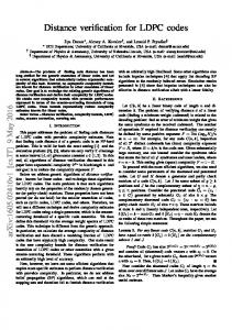
Let R < 1 be a given rational positive number and R(θ) be the random-coding normalized spectrum corresponding to the rate R. Then for any ² > 0 there exists a number d0 > 0 such that: B(θ) < R(θ) + ²
(18)
for all θ ∈ Jδ , and all c, d satisfying d > d0 and R = 1 − c/d. The proof of this theorem is provided in Appendix B.4. Figure 3 presents the set Jδ for a ternary alphabet. The x and y axis represent variables (θ1 , θ2 ) with θ0 being implied by the relation θ0 = 1 − θ1 − θ2 . A triangle outlines the region of valid values for (θ1 , θ2 ) (that is θ1 , θ2 ≥ 0 and θ1 + θ2 ≤ 1). Figure 4 presents the normalized spectrums of a ternary (3, 6)-regular LDPC code (the upper surface) and of the ternary rate 1/2 random-coding ensemble (the lower surface). The normalized spectrums are plotted as functions of parameters (θ1 , θ2 ), with θ0 = 1 − θ1 − θ2 . The above theorem provides uniform convergence only in a subset of the space of valid values of θ. This means that the maximum α (see (13)), evaluated over all values of θ, may be large regardless of the values of c and d. The solution to this problem follows in lines analogous to the binary case. We begin with the following lemma. Lemma 1 Let w be a word of weight l > 0 (l non-zero elements). We now bound the probability of w being a codeword of a randomly selected code, C, of the (c, d)-regular modulo-q ensemble, C. 11
1. if l < d2 N then
Ã
Pr[w ∈ C] ≤
jLk
!µ
lc 2
lc 2L
¶lc
(19)
where L = dc N is the number of check nodes in the parity-check matrix of a (c, d)-regular code and bxc denotes the largest integer smaller than or equal to x. 2. For all l, assuming prime q Pr[w ∈ C] ≤ (cN + 1)q q N (1−R) log A(λ)
(20)
∆
where λ = l/N , A(λ) is given by ∆
A(λ) =
o d 1n 1 + (q − 1)[1 − 2(1 − ρ)λ(1 − λ)] 2 q
(21)
and ρ is some constant dependent on q alone satisfying ρ < 1. The proof of this lemma is provided in Appendix B.5. We now build on this lemma to examine the probability of there being any low-weight words in a randomly selected code for an LDPC ensemble. Theorem 6 Let R = 1 − c/d be fixed, c ≥ 3 and assume q is prime. Then there exists γ > 0, dependent on R and q alone, such that Pr[dmin ≤ γN ] = O(N 1−c/2 )
(22)
where dmin is the minimum distance of a randomly selected (c, d)-regular modulo-q code of length N 1. The proof of this theorem is provided in Appendix B.6. Given an ensemble C of (c, d)-regular LDPC codes of length N and an arbitrary number δ > 0, we define the expurgated ensemble C x as the ensemble obtained by removing all codes of minimum-distance less than or equal to δN from C. If δ ≤ γ (where γ is given by Theorem 6) and N is large enough, this does not reduce the size of the ensemble by a factor greater than 2. Thus the expurgated ensemble average spectrum satisfies: x
S t = 0,
0 < wt(t) ≤ δN
x
wt(t) > δN
S t ≤ 2S t , 1
(23)
In fact, it can be shown that fixing R = 1 − c/d and letting c, d → ∞, the minimum distance of a randomly
selected code is, with high probability, lower bounded by a value arbitrarily close to the Varshamov-Gilbert bound.
12
where wt(t) is the number of nonzero elements in a word of type t. That is, wt(t) =
Pq−1
i=1 ti
=
N − t0 . We refer to the MQC ensemble corresponding to an expurgated (c, d)-regular ensemble as an expurgated MQC-LDPC ensemble. Theorem 7 Let p[y|u] be the transition probability assignment of a discrete memoryless channel with an input alphabet {0, ..., A − 1}. Assume q is prime. Let R be some rational positive number, and let Q(a), δ(x) and N be defined as in Theorem 3. Let ²1 , ²2 > 0 be two arbitrary numbers. ˆx Then for d and N large enough there exists a (c, d)-regular expurgated MQC-LDPC ensemble D (containing all but a diminishingly small proportion of the (c, d)-regular MQC-LDPC codes, as shown in Theorem 6) of length N and design rate R, satisfying R = 1 − c/d, such that the ML x ˆ x satisfies: decoding error probability P e over D x
P e ≤ q −N EQ (R+²1 ) +
q−1 X
(1−²2 )N
Dk
(24)
k=1
The proof of this theorem is provided in Appendix B.7. Applying the same arguments as with BQC-LDPC codes, we obtain that MQC-LDPC codes can be designed for reliable transmission (under ML decoding) at any rate below capacity. Furthermore, at rates approaching capacity, equation (24) is dominated by the random-coding error exponent. Producing bounds for individual MQC-LDPC code ensembles, similar to those provided in Figures 2 and 5, is difficult due to the numerical complexity of evaluating (13), for large q, over sets Jδ given by (17). Note: In our constructions, we have restricted ourselves to prime values of q. In Appendix B.8 we show that this restriction is necessary, at least for values of q that are multiples of 2.
IV
Quantized Coset LDPC Codes over GF(q) (GQC)
We begin by extending the definition of LDPC codes to a finite field GF(q) 2 . In our definition of modulo-q LDPC codes in Section III, the enlargement of the code alphabet size did not extend to the parity-check matrix. The parity-check matrix was designed to contain binary digits alone (with rare exceptions involving parallel edges). We have seen in Appendix B.8 that for nonprime q, this construction results in codes that are bounded away from the random-coding spectrum. The ideas presented in Appendix B.8 are easily extended to ensembles over GF(2m ) for m > 1. 2
Galois fields GF(q) exist for values of q satisfying q = pm where p is prime and m is an arbitrary positive
integer. See [3].
13
We therefore define the GF(q) parity-check matrix differently, employing elements from the entire GF(q) field. Bipartite (c, d)-regular graphs for LDPC codes over GF(q) are constructed in the same way as described in Sections II and III, with the following addition: At each edge (v, c), a random, uniformly distributed label gv,c ∈ GF(q)\{0} is selected. A word x is a codeword if at each check node c the following equation holds: X
gv,c xv = 0
v∈N (c)
where N (c) is the set of variable nodes adjacent to c. The mapping from the bipartite graph to the parity-check matrix proceeds as follows: Element Ai,j in the matrix, corresponding to the ith check node and the jth variable node, is set to the GF(q) sum of all labels ge corresponding to edges connecting the two nodes. As before, the rate of each code is lower bounded by the design rate R = 1 − L/N = 1 − c/d q-ary symbols per channel use. GF(q) coset-ensembles and quantization mappings are defined in the same way as with moduloq codes. Thus we obtain GF(q) quantized coset (GQC) code ensembles. As with MQC codes, analysis of ML decoding properties of GQC LDPC codes involves the types rather that the weights of codewords. Nevertheless, the analysis is simplified using the following lemma: Lemma 2 Let w(1) and w(2) be two equal weight words. The probabilities of the words belonging to a randomly selected code C from a GF(q), (c, d)-regular ensemble satisfy: Pr[w(1) ∈ C] = Pr[w(2) ∈ C] The proof of this lemma relies on the following two observations. First, by the symmetry of the construction of the LDPC ensemble, any reordering of a word’s symbols has no effect on the probability of the word belonging to a randomly selected code. Second, if we replace a nonzero symbol a by another a0 , we can match any code C ∈ C with a unique code C 0 ∈ C such that the modified word belongs to C 0 if and only if the original word belongs to C. The code C 0 is constructed by modifying the labels on the edges adjacent to the corresponding variable node using g 0 = a · g/a0 (evaluated over GF(q)). We have now obtained that the probability of a word belonging to a randomly selected code is dependent on its weight alone, and not on its type. We use this fact in the following theorem, to produce a convenient expression for the normalized spectrum of LDPC codes over GF(q). 14
Theorem 8 The asymptotic normalized ensemble spectrum of a (c, d)-regular LDPC code over GF (q) is given by: B(θ) = H(θ) − cH(λ) − cλ log(q − 1) + (1 − R) log
inf
sgn(x)=sgn(λ)
A(x) xdλ
(25)
where λ = 1 − θ0 and A(x) is given by A(x) =
o 1n [1 + (q − 1)x]d + (q − 1)[1 − x]d q
(26)
Note that in (25) the parameter λ is implied by the relation λ = 1 − θ0 and therefore the right hand side of the equation is in fact a function of θ alone. The proof of the theorem is provided in Appendix C.1. Theorems 3, 5, 6 and Lemma 1 carry over from MQC-LDPC to GQC-LDPC codes, with minor modifications. In Theorem 3, modulo-q addition is replaced by addition over GF(q). In Theorem 5, the requirement q > 2 is added and the definition of Jδ is replaced by Jδ = {(θ0 , ..., θq−1 ) :
0 ≤ θ0 ≤ 1 − δ,
θi ≥ 0 i = 1, ..., q − 1,
q−1 X
θi = 1}
(27)
i=0
The proof is similar to the case of MQC-LDPC codes, setting x = 1/(q − 1) · λ/(1 − λ) in (25) to upper bound B(θ). In Lemma 1, (20) is replaced by ˜
Pr[w ∈ C] ≤ (cN + 1)q N (1−R) log A(λ) ∆ ˜ where λ = l/N and A(λ) is given by ∆ 1 ˜ A(λ) = q
(
·
¸d )
q 1 + (q − 1) 1 − λ q−1
Finally, Theorem 6 carries over unchanged from MQC-LDPC codes. The definition of expurgated GQC-LDPC ensembles is identical to the equivalent MQC-LDPC definition. We now state the main theorem of this section (which is similar to Theorem 7). Theorem 9 Let p[y|u] be the transition probability assignment of a discrete memoryless channel with an input alphabet {0, ..., A − 1}. Suppose q > 2. Let R be some rational positive number, and let Q(a), δ(x) and N be defined as in Theorem 3. Let ² > 0 be an arbitrary number. Then for d and ˆ x (containing all N large enough there exists a (c, d)-regular expurgated GQC-LDPC ensemble D but a diminishingly small proportion of the (c, d)-regular GQC-LDPC codes, as shown in Theorem 6) of length N and design rate R, satisfying R = 1 − c/d, such that the ML decoding error x ˆ x satisfies: probability P e over D x
P e ≤ q −N EQ (R+²) 15
(28)
The proof of this theorem follows in the lines of Theorem 7, replacing (78) with ∆
U = {t ∈ T : 0 < wt(t) ≤ δN }
(29)
The difference between (28) and (24) results from the larger span of the set Jδ defined in (27) in comparison with the one defined in Theorem 5. Thus we are able to define U such that the first term in (12) disappears. Applying the same arguments as with BQC-LDPC codes and MQC-LDPC codes, we obtain that GQC-LDPC codes can be designed for reliable transmission (under ML decoding) at any rate below capacity. Furthermore, the above theorem guarantees that at any rate, the decoding error exponent for GQC-LDPC codes asymptotically approaches the random-coding exponent, thus outperforming our bounds for both the BQC-LDPC and MQC-LDPC ensembles. Figure 5 compares several GQC-LDPC code ensembles over the AWGN channel. The quantizations used are the same as those used for Figure 2 and are given by (10) (using the representation of elements of GF(2m ) by m-dimensional binary vectors [3]). To obtain these bounds, we again use methods similar to the ones discussed above for BQC-LDPC codes (here we seek the maximum δ such that S θ N Dθ N → 0 for all θ having wt(θN ) ≤ δN and then define U as in (29)).
V
Iterative decoding
Our analysis so far has focused on the desirable properties of the proposed codes under optimal maximum-likelihood (ML) decoding. In this section we demonstrate that the various codes show favorable performance also under practical iterative decoding. The BQC-LDPC belief propagation decoder is based on the well-known LDPC decoder, with differences involving the addition of symbol nodes alongside variable and check nodes, derived from a factor graph representation by McEliece [20]. The decoding process attempts to recover c, the codeword of the underlying LDPC code. Figure 6 presents an example of the bipartite graph for a (2, 3)-regular BQC-LDPC code with T = 3. Variable nodes and check nodes are defined in a manner similar to that of standard LDPC codes. Symbol nodes correspond to the symbols of the quantized codeword (1). Each symbol node is connected to the T variable nodes that make up the sub-vector that is mapped to the symbol. Decoding consists of alternating rightbound and leftbound iterations. In a rightbound iteration, messages are sent from variable nodes to symbol nodes and check nodes. In a leftbound iteration, the opposite occurs. Unlike the standard LDPC belief-propagation decoder, the channel output
16
“resides” at the symbol nodes, rather than at the variable nodes. The use of the coset vector is easily accounted for at the symbol nodes. The MQC-LDPC and GQC-LDPC belief propagation decoders are modified versions of the belief propagation decoder introduced by Gallager in [12] for arbitrary alphabet LDPC codes, employing q-dimensional vector messages. The modifications, easily implemented at the variable nodes, account for the addition of the coset vector v at the transmitter and for the use of quantization. Efficient implementation of belief propagation decoding of arbitrary-alphabet LDPC codes is discussed by Davey and MacKay [8] and by Richardson and Urbanke [23]. The ideas in [8] are suggested in the context of LDPC codes over GF(q) but also apply to codes employing modulo-q arithmetic. The method discussed in [23] suggests using the DFT (the m dimensional DFT for codes over GF(pm )) to reduce complexity. This is particularly useful for codes defined over GF(2m ), since then the multiplications are eliminated. An important property of quantized coset LDPC codes (BQC, MQC and GQC) is that for any given bipartite graph, the probability of decoding error, averaged over all possible values of the coset vector v, is independent of the transmitted codeword c of the underlying LDPC code (as observed by Kav˘ci´c et al. [15] in the context of coset LDPC codes for ISI channels). This facilitates the extension of the density evolution analysis method (see [23]) to quantized coset codes. BQC-LDPC density evolution evaluates the density of messages originating from symbol nodes using Monte-Carlo simulations. Density evolution for MQC and GQC-LDPC codes is complicated by to the exponential amount of memory required to store the probability densities of q-dimensional messages. A possible solution to this problem is to rely on Monte-Carlo simulations to evolve the densities.
V.1
Simulation Results for BQC-LDPC Codes
In this paper, we have generally confined our discussion to LDPC codes based on regular graphs. Nevertheless, as with standard LDPC codes, the best BQC-LDPC codes under belief-propagation decoding are based on irregular graphs as introduced by Luby et al. [18]. In this section we therefore focus on irregular codes. A major element in generating good BQC-LDPC codes is the design of good quantizations. In our analysis of ML decoding, we focused on the probability assignment Q(a) associated with the quantizations. A good probability assignment for memoryless AWGN channels is generally designed to approximate a Gaussian distribution (see [30] and [31]). Iterative decoding, however, 17
is sensitive to the particular mapping δ(x). A key observation in the design of BQC-LDPC quantizations is that the degree of error protection provided to different bits that are mapped to the same channel symbol, is not identical. Useful figures of merit are the following values (adapted from [24][Section III.E], replacing the log-likelihood messages of [24] with plain likelihood messages): s
∆l =
1 E 2
X (l) 1 − X (l)
l = 1, ..., T
(30)
where X (l) is a random variable corresponding to the leftbound message from the lth position of a symbol node, assuming the transmitted symbol was zero, in the first iteration of belief propagation. It is easy to verify that the following relation holds ∆l = Γl1 =
1 Xq l l Γ1 Γ0 2T y X
Pr[y | δ(v)],
v:vl =1
Γl0 =
X
Pr[y | δ(v)]
v:vl =0
Quantizations rendering a low ∆l for a particular l produce a stronger leftbound message at the corresponding position, at the first iteration. Given a particular distribution Q(a), different quantizations δ(x) associated with Q(a) produce different sets {∆l }Tl=1 . In keeping with the experience available for standard LDPC codes, simulation results indicate that good quantizations favor an irregular set of {∆l }Tl=1 , meaning that some values of the set are allowed to be larger than others. In the design of edge distributions, to further increase irregularity, it is useful to consider not only the fraction λi of edges of given left-degree i but rather λi,l , accounting for the left variable node’s symbol node position. In this paper we have employed only rudimentary methods of designing BQC-LDPC edge distributions. Table 1 presents the edge distributions of a rate 2 (measured in bits per channel use) BQC-LDPC code for the AWGN channel. The following length T = 4 quantization was used with 8-PAM signaling (A = 8). Applying the notation of (10), we obtain that a simple assignment of values in an ascending order renders a good quantization. δ = [−1.94, −1.39, −0.832, −0.832, −0.832, −0.277, −0.277, −0.277, 0.277, 0.277, 0.277, 0.832, 0.832, 0.832, 1.39, 1.94] The SNR threshold (determined by simulations) is 1.1 dB away from the Shannon limit (which is 11.76 dB at rate 2) at a block length of Nb = 200, 000 bits or N = 50, 000 symbols and a bit error rate of about 10−5 . Decoding typically requires 100-150 iterations to converge. Note that 18
the ML decoding threshold of a random code, constructed using the distribution Q(a) associated with δ(x), is 11.99 dB (evaluated using the mutual information as described in [13][Section 5.6]). Thus the gap to the random-coding limit is 0.87 dB. The edge distributions were designed based on a rate 0.5 binary LDPC code suggested by [24], using trial-and-error to design {λi,l } while keeping the marginal distribution {λi } fixed.
V.2
Simulation Results for MQC-LDPC Codes
The MQC equivalent of (30) are the values {Di }q−1 i=0 given by equations (11). As with BQC-LDPC codes, MQC-LDPC codes favor quantizations rendering an irregular set {Di }q−1 i=0 (as indicated by simulation results). In [24] and [6], methods for the design of edge distributions are presented that use singleton error probabilities produced by density evolution and iterative application of linear programming. In this work we have used a similar method, replacing the probabilities produced by density evolution with results of Monte-Carlo simulations. An additional improvement was obtained by replacing singleton error probabilities by the functional Eh(X) (h denoting q-ary entropy). Table 2 presents the edge distributions of a rate 2 (measured again in bits per channel use) MQC-LDPC code for the AWGN channel. The code alphabet size is q = 17, and 9-PAM signaling was used (A = 9), with the quantization listed below. The values of δ(x) are listed in ascending order, i.e. [δ(0), δ(1), ..., δ(16)]. The quantization values were selected to approximate a Gaussian distribution, and their order was determined by trial-and-error. δ = [0, 0.972, 1.46, −0.486, 0.486, 0, −0.972, 0.486, −1.94, 0, −0.972, −0.486, 0.972, −0.486, 0.486, 1.94, −1.46] At an SNR 0.9 dB away from the Shannon limit, the symbol error rate was 5.5 · 10−5 (50 Monte Carlo simulations). The gap to the ML decoding threshold of a random code, constructed using the distribution Q(a) associated with δ(x), is 0.7 dB. The block length used was N = 50, 000 symbols or Nb = 204, 373 bits. Decoding typically required 100-150 iterations to converge.
V.3
Simulation Results for GQC-LDPC Codes
In contrast to BQC-LDPC and MQC-LDPC codes, GQC-LDPC appear resilient to the ordering of values in the quantizations used. This is the result of the use of random labels, which infer a permutation on the rightbound and leftbound messages at check nodes.
19
Table 3 presents the edge distributions of a rate 2 (measured again in bits per channel use) GQC-LDPC code for the AWGN channel. The methods used to design the codes are the same as those described above for MQC-LDPC codes. The code alphabet size is q = 16, and 9-PAM signaling was used (A = 9), with the quantization listed below. The values of δ(x) are listed in ascending order (using the representation of elements of GF(2m ) by m-dimensional binary vectors [3]). The quantization values were selected to approximate a Gaussian distribution. δ = [−1.9, −1.42, −0.949, −0.949, −0.475, −0.475, −0.475, 0, 0, 0, 0.475, 0.475, 0.949, 0.949, 1.42, 1.9] At an SNR 0.65 dB away from the Shannon limit, the symbol error rate was less than 10−5 (100 Monte Carlo simulations). The gap to the ML decoding threshold of a random code, constructed using the distribution Q(a) associated with δ(x), is 0.4 dB. The block length used was N = 50, 000 symbols or Nb = 200, 000 bits. Decoding typically required 100-150 iterations to converge.
V.4
Comparison with existing methods
Wachsmann et al. [31], present reliable transmission using multilevel codes with Turbo Code constituent codes, at approximately 1 dB of the Shannon limit at rate 1 bit per dimension. Multilevel coding is similar to BQC quantization mapping, in that multiple bits (each from a separate binary code) are combined to produce channel symbols. However, the division of the code into independent subcodes and the hard decisions performed during multistage decoding, are potentially suboptimal. Robertson and W¨orts [25], using Turbo Codes with TCM constituent codes, report several results that include reliable transmission within 0.8 dB of the Shannon limit at rate 1 bit per dimension. Kav˘ci´c, Ma, Mitzenmacher and Varnica [16], [19] and [29] present reliable transmission at 0.74 dB of the Shannon limit at rate 2.5 bits per dimension. Their method has several similarities to BQC-LDPC codes. As in multilevel schemes, multiple bits from the outer codes are combined and mapped into channel symbols in a manner similar to BQC quantizations. Quantization mapping can be viewed as a special case of a one-state MIR trellis code, having 2T parallel branches connecting every two subsequent states of the trellis. Furthermore, the irregular LDPC construction method of [19] and [29] is similar to the method of Section V.1. In [19] and [29], the edge distributions for the outer LDPC codes are optimized separately, and the resulting codes are interleaved into one LDPC code. Similarly, BQC-LDPC construction distinguishes 20
between variable nodes of different symbol node position. However, during the construction of the BQC-LDPC bipartite graph, no distinction is made between variable nodes in the sense that all variable nodes are allowed to connect to the same check nodes (see Section II). This contrasts the interleaved LDPC code of [19] and [29], where variable nodes originating from different subcodes are connected to distinct sets of check nodes.
VI
Conclusion
The codes presented in this paper provide a simple approach to the problem of applying LDPC codes to arbitrary discrete memoryless channels. Quantization mapping (based on ideas by Gallager [13] and McEliece [20]) has enabled the adaptation of LDPC codes to channels where the capacity-achieving source distribution is nonuniform. It is thus a valuable method of overcoming the shaping gap to capacity. The addition of a random coset vector (based on ideas by Gallager [13] and Kav˘ci´c et al. [15]) is a crucial ingredient for rigorous analysis. Our focus in this paper has been on ML decoding. We have shown that all three code configurations presented, under ML decoding, are capable of approaching capacity arbitrarily close. Our analysis of MQC and GQC codes has relied on generalizations of concepts useful with binary codes, like code spectrum and expurgated ensembles. We have also demonstrated the performance of practical iterative decoding. The simple structure of the codes presented lends itself to the design of conceptually simple decoders, which are based entirely on the well-established concepts of iterative belief-propagation (e.g. [20], [22], [12]). We have presented simulation results of promising performance within 0.65 dB of the Shannon Limit at rate 2 bits per channel use. We are currently working on an analysis of iterative decoding of quantized coset LDPC codes [1].
Appendix A A.1
Proofs for Section II Proof of Dx < 1 for x 6= 0 for non-degenerate quantizations and channels
We define a quantization to be non-degenerate if there exists no integer n > 1 such that Q(a)·2T is an integer multiple of n for all a (such a quantization could be replaced by a simpler quantization over an alphabet of size 2T /n that would equally attain input distribution Q(a)). A channel is non-degenerate if there exist no values a1 , a2 ∈ {0, ..., A − 1} such that Pr[y | a1 ] = Pr[y | a2 ] 21
for all y. By inspecting when the Cauchy-Schwartz inequality becomes an equality, we see that Dx = 1 (x 6= 0) if and only if Pr[y|δ(ξ)] = Pr[y|δ(ξ ⊕ x)] for all y and ξ. Hence, by the channel non-degeneracy assumption, δ(ξ) = δ(ξ ⊕ x), for all ξ. This contradicts the quantization nondegeneracy assumption, since the number of elements in {0, 1}T that are mapped to each channel symbol is some integer multiple of the additive order of x (which is two).
A.2
Sketch of Proof for Theorem 1
The proofs of Theorems 1 and 3 are similar. In this paper we have selected to elaborate on Theorem 3, as the gap between its proof and proofs provided in [26] and [21] is greater. Thus we concentrate here only on the differences between the two. U
Uc
U
Uc
As in Appendix B.1, we define P e|m,Cˆ and P e (and equivalently P e|m,Cˆ and P e ) as U
P e|m,Cˆ U
Pe
ˆ ˆm ) ∈ U | m was transmitted, C} = Pr{y : ∃m0 6= m : Pr[y|δ(ˆ cm0 )] ≥ Pr[y|δ(ˆ cm )], wt(ˆ cm0 ⊕ c XX 1 ˆ · PU ˆ = Pr[C] e|m,C M m ˆ C
ˆ defined as in Definition 1. We obtain (using the union bound): where Cˆ is a code of ensemble C, Uc
U
Pe ≤ Pe + Pe
(31)
We proceed to bound both elements of the sum: 1. As in Appendix B.1 we obtain: U Pe|m, ˆ C
Xq
X
≤
m0 :wt(ˆ c
Pr[y|δ(ˆ cm0 )] Pr[y|δ(ˆ cm )]
cm )∈U y m0 ⊕ˆ
∆
ˆm,i = < cˆm,(i−1)T +1 , ..., cˆm,iT > we obtain the following identity: Recalling (1) and defining c δ(ˆ cm ) =< δ(ˆ cm,1 ), ..., δ(ˆ cm,N ) > Each element yi of the vector y is now dependent only on the transmitted symbol δ(ˆ cm,i ) at position i. We therefore obtain U Pe|m, ˆ C
≤
X
N q XY
Pr[yi |δ(ˆ cm0 ,i )] Pr[yi |δ(ˆ cm,i )]
cm )∈U y i=1 m0 :wt(ˆ cm0 ⊕ˆ
=
X
N Xq Y
Pr[y|δ(ˆ cm0 ,i )] Pr[y|δ(ˆ cm,i )]
cm )∈U i=1 y m0 :wt(ˆ cm0 ⊕ˆ
22
U
Using the above result, we now examine P e|m,C 0 , the probability of error for a fixed parent code C 0 (obtained by step 1 of Definition 1), averaged over all possible values of v. U P e|m,C 0
N Y
X
≤
m0 :wt(c0m0 ⊕c0m )∈U
Evi
Xq
Pr[y|δ(c0m0 ,i ⊕ vi )] Pr[y|δ(c0m,i ⊕ vi )]
y
i=1
ˆm,i . Letting c ˜m0 ,i = vi and c0m,i are defined in a manner similar to the definition of c ˜ i = vi ⊕ c0m,i we obtain: c0m0 ,i ⊕ c0m,i and v U
P e|m,C 0
N Y
X
≤
Ev˜ i
Xq
N Y
X
=
˜ i )] Pr[y|δ(˜ vi )] Pr[y|δ(˜ cm0 ,i ⊕ v
y
m0 :wt(˜ cm0 )∈U i=1
Dc˜m0 ,i
(32)
m0 :wt(˜ cm0 )∈U i=1
where Dc˜m0 ,i is defined as in (2). Defining lm0 = wt(˜ cm0 ) we observe that at least dlm0 /T e of the components {˜ cm0 ,i } are not equal to 0, and hence, recalling (3), U
P e|m,C 0
X
≤
m0 :lm0 ∈U
=
X
X
Ddlm0 /T e ≤
Dlm0 /T
m0 :lm0 ∈U
Sl0 Dl/T
l∈U
where Sl0 is the spectrum of code C 0 . Clearly this bound can equally be applied to Pe|C 0 , abandoning the assumption of a fixed m. The average spectrum of ensemble C 0 is equal to that of our original ensemble C, and therefore we obtain U
U P e = EC 0 {Pe|C 0} ≤
X
S l Dl/T
(33)
l∈U
2. The methods used to bound the second element of (31) are similar to those used in Appendix B.1. The bound obtained is Uc
P e ≤ 2−N EQ (R+log α/N )
(34)
Combining (31), (33) and (34) we obtain our desired result of (4). 2
A.3
Proof of Theorem 2
Let γ be defined as in (7). Let δ be some arbitrary number smaller than γ that will be determined ˆ x , obtained by expurgating codes later. Let C x be the underlying expurgated LDPC ensemble of D x
with minimum distance less than or equal to δN . We use Theorem 1 to bound P e . 23
Defining U0 = {1, ..., δN T } U1 = {(1 − δ/2)N T, ..., N T } U we have (using (4)) x
Pe ≤
= U0 ∪ U1
X x S l Dl/T + 2−N EQ (R+(log α)/N )
(35)
l∈U
We now examine both elements of the above sum. 1. Given that all codes in the expurgated ensemble have minimum distance greater than δN T , x
we obtain that S l = 0 for all l ∈ U0 . We therefore turn to examine U1 . A desirable effect of expurgation is that it also reduces the number of words having large l. Assume c1 and c2 are two codewords of a code C x ∈ C x , such that their weight satisfies ∆
l ≥ (1 − δ/2)N T . The weight of the codeword c0 = c1 ⊕ c2 satisfies l ≤ δN T , contradicting the construction of the expurgated ensemble. Hence, C x cannot contain more than one T x codeword having l ∈ U1 . Letting {Slx }N l=1 denote the spectrum of code C , we have
X
Slx Dl/T ≤ 1 · D(1−δ/2)N T /T = D(1−δ/2)N
l∈U
Clearly this average carries over to the average spectrum. Selecting δ so that δ/2 ≤ ²2 we obtain:
X x S l Dl/T ≤ D(1−²2 )N
(36)
l∈U
2. Examining the proof by [21][Appendix E], we obtain ³ ´ o(N T ) log α R ≤ (1 − ) log 1 + (1 − 2δ/2)d + NT T NT
Therefore, there exist positive integers N0 and d0 such that for c, d, N satisfying R = 1−c/d, d > d0 and N > N0 the following inequality holds: 1 log α < ²1 N Combining (35), (36) and (37) we obtain our desired result of (9). 2
24
(37)
B
Proofs for Section III
B.1
Proof of Theorem 3
The proof of this theorem is a generalization of the proofs available in [21] and [26], from binaryinput symmetric-output to arbitrary channels. ˆ in D ˆ have the form {δ(ˆ ˆ for some code Cˆ of C. ˆ We can therefore ˆm ∈ C} All codes D cm ) : c write: Pe =
XX 1 m
ˆ C
M
ˆ ·P Pr[C] ˆ e|m,C
where ˆ P e|m,Cˆ = Pr{y : ∃m0 6= m : Pr[y|δ(ˆ cm0 )] ≥ Pr[y|δ(ˆ cm )] | m was transmitted, C} U
Uc
U
Uc
We define P e|m,Cˆ and P e (and equivalently P e|m,Cˆ and P e ) as U
ˆ ˆm ) ∈ U | m was transmitted, C} = Pr{y : ∃m0 6= m : Pr[y|δ(ˆ cm0 )] ≥ Pr[y|δ(ˆ cm )], type(ˆ cm0 − c XX 1 ˆ · PU ˆ (38) = Pr[C] e|m,C M m ˆ
P e|m,Cˆ U
Pe
C
and obtain (using the union bound): Uc
U
Pe ≤ Pe + Pe
(39)
We now proceed to bound both elements of the sum: U
1. We first bound P e|m,Cˆ (defined above), the error probability for a fixed index m and code ˆ This is the probability that some codeword c ˆm0 such that type(ˆ ˆm ) ∈ U is more C. cm0 − c ˆm . likely to have produced the observation y than the true c U
P e|m,Cˆ
ˆ ˆm ) ∈ U | m was transmitted, C} = Pr{y : ∃m0 6= m : Pr[y|δ(ˆ cm0 )] ≥ Pr[y|δ(ˆ cm )], type(ˆ cm0 − c =
X
I(y) Pr[y|δ(ˆ cm )]
y
where I(y) is defined as follows: (
I(y) =
ˆm ) ∈ U 1 ∃m0 6= m : P r[y|δ(ˆ cm0 )] ≥ Pr[y|δ(ˆ cm )], type(ˆ cm0 − c 0
otherwise
Therefore: U P e|m,Cˆ
≤
X
I(y) Pr[y|δ(ˆ cm )]
y
X cm )∈U m0 :type(ˆ cm0 −ˆ
25
s
Pr[y|δ(ˆ cm0 )] Pr[y|δ(ˆ cm )]
≤
X
Pr[y|δ(ˆ cm )]
y
m0 :type(ˆ cm0 −ˆ cm )∈U
Xq
X
=
m0 :type(ˆ c
Pr[y|δ(ˆ cm0 )] Pr[y|δ(ˆ cm )]
Pr[y|δ(ˆ cm0 )] Pr[y|δ(ˆ cm )]
cm )∈U y m0 −ˆ N q XY
X
=
s
X
Pr[yi |δ(ˆ cm0 ,i )] Pr[yi |δ(ˆ cm,i )]
m0 :type(ˆ cm0 −ˆ cm )∈U y i=1 N Xq Y
X
=
Pr[y|δ(ˆ cm0 ,i )] Pr[y|δ(ˆ cm,i )]
m0 :type(ˆ cm0 −ˆ cm )∈U i=1 y
Each code Cˆ has the form {c + v : c ∈ C} for some parent code C ∈ C and a vector v. We U
now use the above result to bound P e|m,C , the probability of error for a fixed parent code C, averaged over all possible values of v. U
P e|m,C
X
=
v
U U Pe|m,C,v Pr[v] = Ev {Pe|m,C,v } N Xq Y
X
≤ Ev {
Pr[y|δ(cm0 ,i + vi )] Pr[y|δ(cm,i + vi )] }
m0 :type(cm0 −cm )∈U
i=1 y
The elements of the random vector v are N i.i.d. random variables {vi }N i=1 . Therefore U P e|m,C
N Y
X
≤
m0 :type(c
m0 −cm )∈U
Evi
Xq
Pr[y|δ(cm0 ,i + vi )] Pr[y|δ(cm,i + vi )]
y
i=1
Letting c˜m0 ,i = cm0 ,i − cm,i and v˜i = vi + cm,i we obtain: U
P e|m,C
≤
N Y
X
Ev˜i
N Y
X
Pr[y|δ(˜ vi )] Pr[y|δ(˜ cm0 ,i + v˜i )]
y
m0 :type(˜ cm0 )∈U i=1
=
Xq
Dc˜m0 ,i
m0 :type(˜ cm0 )∈U i=1
where Dc˜m0 ,i is defined as in (11). Letting tm0 = type(˜ cm0 ), we have: U
P e|m,C
≤
X
Dtm0
m0 :tm0 ∈U
=
X
St Dt
t∈U
Clearly this bound can equally be applied to Pe|C , abandoning the assumption of a fixed m. U
Finally, we bound P e : U
U P e = EC {Pe|C }≤
X
S t Dt
t∈U Uc
2. We now bound P e . For this we define a set of auxiliary ensembles. 26
(40)
(a) Ensemble C 0 is generated from C by adding, for each code C in C, the codes generated by all possible permutations on the order of codewords within the code. (b) Ensemble C 00 is generated from C 0 by adding, for each code C 0 in C 0 , the codes generated by all possible permutations σ on the order of symbols within the code. (c) Ensemble C˜ is generated from C 00 by adding, for each code C 00 in C 00 , codes Cv00 of the form {c00 + v|c00 ∈ C 00 } for all possible vectors v ∈ {0, ..., q − 1}N . Examining the above construction, it is easy to verify that any reordering of the steps has no impact on the final result. Therefore ensemble C˜ can be obtained from Cˆ by employing steps 2a and 2b. ˜ as the quantization of C. ˜ D ˜ can equivalently be obtained emWe also define ensemble D c
ˆ Therefore P U ploying the above steps 2a and 2b on ensemble D. e , defined based on (38), is c ˜ identical to a similarly defined P˜eU , evaluated over ensemble C.
Uc We proceed to examine P˜e|m Uc P˜e|m =
X ˜ C
=
c
˜ · P˜ U ˜ Pr[C] e|m,C
XX y
x0
Uc Pr[˜ cm = x0 ] · Pr[y | δ(x0 )] · P˜e|m,x 0 ,y
(41)
Uc ˜m = x0 , where P˜e|m,x is defined as the probability, for a fixed y and index m, assuming c 0 ,y
˜m ) ∈ U c should be more likely than that a codeword of the form δ(˜ cm0 ), where type(˜ cm0 − c the transmitted δ(˜ cm ). The random space here consists of a random selection of the code ˜ Therefore: C˜ from C. Uc ˜m ) ∈ U c | c ˜m = x0 } P˜e|m,x = Pr{∃m0 6= m : Pr[y|δ(˜ cm0 )] ≥ Pr[y|δ(˜ cm )], type(˜ cm0 − c 0 ,y
˜m0 = x1 | c ˜m = x0 } = Pr{∃m0 6= m, ∃x1 : Pr[y|δ(x1 )] ≥ Pr[y|δ(x0 )], type(x1 − x0 ) ∈ U c , c Letting 0 ≤ ρ ≤ 1 be an arbitrary number, we have by the union bound (extended as in [13])
ρ
X
X
Uc P˜e|m,x ≤ 0 ,y
m0 6=m
˜m = x0 ] Pr[˜ cm0 = x1 | c
x1 :Pr[y|δ(x1 )]≥Pr[y|δ(x0 )], type(x1 −x0 )∈U c
Employing Lemma 3, which is provided in Appendix B.2, we obtain
ρ
X
Uc ≤ (M − 1) P˜e|m,x 0 ,y
x1 :Pr[y|δ(x1 )]≥Pr[y|δ(x0 )], type(x1 −x0 )∈U c
27
αq −N
ρ
X
≤ (M − 1)α
q
X
= (M − 1)α
QN
i=1 Q(ui ),
q −N
x1 :δ(x1 )=u1
we have:
ρ
X
Uc
P˜e|m,x0 ,y ≤ (M − 1)α
Q(u1 )
u1 :Pr[y|u1 ]≥Pr[y|δ(x0 )]
µ
X
≤ (M − 1)α
Q(u1 )
u1 :Pr[y|u1 ]≥Pr[y|δ(x0 )]
"
≤
ρ
X
u1 :Pr[y|u1 ]≥Pr[y|δ(x0 )]
∆
x1 :Pr[y|δ(x1 )]≥Pr[y|δ(x0 )]
Letting Q(u) =
−N
(M − 1)α
X u1
µ
Pr[y|u1 ] Q(u1 ) Pr[y|δ(x0 )]
Pr[y|u1 ] Pr[y|δ(x0 )]
¶s
ρ
¶s #ρ
where s > 0 is some arbitrary number. Letting u0 = δ(x0 ) we have: " Uc P˜e|m,x 0 ,y
≤ (M − 1)α
X u1
µ
Pr[y|u1 ] Q(u1 ) Pr[y|u0 ]
¶s #ρ
(42)
Using (41) and (42) we obtain: Uc P˜e|m ≤
XX y
"
X
Pr[˜ cm = x0 ] · Pr[y | u0 ] · (M − 1)α
X
u0 x0 :δ(x0 )=u0
u1
µ
Pr[y|u1 ] Q(u1 ) Pr[y|u0 ]
¶s #ρ
Employing Lemma 3 once more, we obtain Uc P˜e|m
≤ α
ρ
XX y
= α
ρ
u0
XX y
X
q
x0 :δ(x0 )=u0
−N
"
· Pr[y | u0 ] · (M − 1)
X u1
"
Q(u0 ) · Pr[y | u0 ] · (M − 1)
u0
X u1
µ
Pr[y|u1 ] Q(u1 ) Pr[y|u0 ]
µ
Pr[y|u1 ] Q(u1 ) Pr[y|u0 ]
¶s #ρ
¶s #ρ
The remainder of the proof follows in direct lines as in [13][Theorem 5.6.1]. Abandoning the c
c U assumption of a fixed m, and recalling that P e = P˜eU , we obtain:
Uc
P e ≤ q −N EQ (R+log α/N ) Combining (39), (40) and (43) we obtain our desired result of (12). 2
28
(43)
B.2
Statement and proof of Lemma 3
The following lemma is used in the proof of Theorem 3 and relies on the notation introduced there. ˜i and Lemma 3 Let x0 , x1 ∈ {0, ..., q − 1}N and let 1 ≤ i, j ≤ M be two distinct indexes. Let c ˜ Then ˜j be the respective codewords of a randomly selected code C˜ of C. c 1. Pr[˜ ci = x0 ] = q −N 2. If type(x1 − x0 ) ∈ U c then Pr[˜ cj = x1 |˜ ci = x0 ] ≤ αq −N
(44)
where α is defined by (13). ˜ We first fix the ancestor code C and investigate Proof. Let C˜ be a randomly selected code from C. the relevant probabilities. We define the following random variables: C 00 denotes the “parent” code from which C˜ was generated. Likewise, C 0 denotes the parent of C 00 , and C denotes the parent of C 0 . Let w be an arbitrary nonzero word. We now examine the codewords of C 0 (
Pr[c0i
−
c0j
1 MC −1
w∈C
0
otherwise
= w | C] =
where MC is the number of codewords in C. Recalling that C is of rate at least R, we have that MC ≥ M and hence 1/(MC − 1) ≤ 1/(M − 1). We now examine C 00 : h
Pr c00i − c00j = w | C
i
=
X
h
i
Pr c0i − c0j = σ −1 (w) | C Pr(σ)
σ
≤ =
h i 1 Pr σ −1 (w) ∈ C M −1 1 St ·¡ N ¢ M − 1 t ,...,t 0
q−1
where t is the type of w. The last equation holds because, given a uniform random selection of the symbol-permutation σ, the probability of σ −1 (w) being a codeword of C is equal to the fraction of t-type C codewords within the entire set of t-type words. Examining C˜ we have: Pr[˜ ci = x0 | C] =
X
Pr[˜ ci = x0 | v, C] · Pr[v] = q −N
X v
v
29
Pr[c00i = x0 − v | C] = q −N
˜i = x0 , C] = Pr[˜ cj = x1 | c
˜i = x0 | C] Pr[˜ cj = x1 , c Pr[˜ ci = x0 | C]
= qN =
X
X
˜i = x0 | C, v] q −N Pr[˜ cj = x1 , c
v
Pr[c00j = x1 − v, c00i = x0 − v | C]
v
=
X
Pr[c00j − c00i = x1 − x0 , c00i = x0 − v | C]
v
1 St ·¡ N M − 1 t ,...,t
= Pr[c00j − c00i = x1 − x0 | C] ≤
0
¢
q−1
where t is now the type of x1 − x0 . We finally abandon the assumption of a fixed C, and obtain: Pr[˜ ci = x0 ] = q −N ˜i = x0 ] ≤ Pr[˜ cj = x1 | c
1 St ·¡ N M − 1 t ,...,t 0
¢
q−1
If t is in U c , we obtain from (13) the desired result of (44), and thus complete the proof of the lemma. 2
B.3
Proof of Theorem 4
To prove this theorem, we first quote the following notation and theorem, by Burshtein and Miller [4] (see also [14]). Given a multinomial p(x1 , ..., xm ), the coefficient of
Q
ni i xi
is denoted3
bp(x1 , ..., xm )n1 ,...,nm c. The theorem is stated for the two dimensional case but is equally valid for higher dimensions (we present a truncated version of the theorem actually discussed in [4]). Theorem 10 Let γ > 0 be some rational number and let p(x, y) be a function such that p(x, y)γ is a multinomial with non-negative coefficients. Let α > 0 and β > 0 be some rational numbers and let ni be the series of all indices j such that j/γ is an integer and bp(x, y)j cαj,βj 6= 0. Then bp(x, y)ni cαni ,βni ≤
p(x, y)ni x>0,y>0 xαni y βni inf
(45)
and lim
i→∞
1 p(x, y) logbp(x, y)ni cαni ,βni = log inf x>0,y>0 ni xα y β
(46)
We now use this theorem to prove Theorem 4. The proof follows in the lines of a similar proof for binary codes in [4]. 3
The same notation bxc is used to denote the largest integer smaller than or equal to x. The distinction between
the two meanings is to be made based on the context of the discussion.
30
We first calculate the asymptotic spectrum for θ satisfying θi > 0 for all i. Given a type t and 1 ≤ j ≤
¡
¢ N t0 ,...,tq−1 ,
let Xtj be an indicator r.v. equal to 1 if the j-th
word of type t (by some arbitrary ordering of type-t words) is a codeword of a drawn code, and 0 otherwise. Then N (t0 ,...,t ) q−1
X
St =
Xtj
j=1
Therefore, N (t0 ,...,t ) q−1
St = E
X
Xtj
N (t0 ,...,t ) q−1
=
j=1
X
EXtj
N (t0 ,...,t ) q−1
X
=
j=1
Ã
Pr[Xtj
j=1
!
N = 1] = Pr[Xt1 = 1] (47) t0 , ..., tq−1
the final equality resulting from the symmetry of the ensemble construction. Thus, for all θ 1 1 log S θ N = H(θ) + lim log Pr[Xθ1 N = 1] N →∞ N N →∞ N lim
(48)
We now examine P r[Xθ1 N = 1]. Let w be a word of type θN . Each assignment of edges by a random permutation infers a symbol “coloring” on each of the check node sockets, using θi N c colors of type i (i = 0, . . . , q − 1). The total number of colorings is: Ã
t(θ; N ) =
Nc θ0 N c, ..., θq−1 N c
!
(49)
Given an assignment of graph edges, w is a codeword if at each check node, the modulo-q sum of all adjacent variable nodes is zero. The number of valid assignments (assignments rendering w a codeword), is determined using an enumerating function: e(θ; N ) = b[A(x0 , ..., xq−1 )](1−R)N cθ N c
(50)
where A(x) is given by Ã
X
A(x) =
(k0 ,...,kq−1 ) : 0≤ki ≤d,
P
ki =d,
P
iki (mod q)=0
!
d kq−1 xk0 · ... · xq−1 k0 , ..., kq−1 0
we now have 1 1 e(θ; N ) log Pr[Xθ1 N = 1] = lim log N →∞ N N →∞ N t(θ; N ) lim
(51)
Using (49) we have lim
N →∞
1 log t(θ; N ) = cH(θ) N 31
(52)
Using (50) and Theorem 10 we have: 1 1 log e(θ; N ) = (1 − R) lim logb[A(x0 , ..., xq−1 )](1−R)N cθ cN N →∞ N N →∞ (1 − R)N 1 = (1 − R) lim logb[A(x0 , ..., xq−1 )]N cθ dN N →∞ N A(x0 , ..., xq−1 ) = (1 − R) log inf dθ x>0 x 0 · ... · xdθq−1 0 q−1 lim
(53)
Combining (48), (51), (52) and (53) we obtain: lim
N →∞
1 A(x) log S θ N = (1 − c)H(θ) + (1 − R) log inf x>0 xdθ N
To adapt the proof to θ having θi = 0 for some i, we modify the expression for e(θ; N ) as follows. Assuming (without loss of generality) that θi 6= 0 for all i ≤ i0 , and θi = 0 for all i > i0 , we obtain: ˜ 0 , ..., xi )](1−R)N c(θ ,...,θ )·cN e(θ; N ) = b[A(x 0 0 i0 ˜ 0 , ..., xi ) is given by where A(x 0 Ã
X
˜ 0 , ..., xi ) = A(x 0 (k0 ...ki0 ) : 0≤ki ≤d,
P
ki =d,
P
iki (mod q)=0
!
d ki xk00 · ... · xi0 0 k0 , ..., ki0
= A(x0 , ..., xi0 , 0...0) Following in the line of previous development, we obtain: 1 log S θ N N →∞ N
B(θ) = lim
= (1 − c)H(θ) + (1 − R) log = (1 − c)H(θ) + (1 − R) log
xo ,...,xi0 >0,
A(x) xi0 +1 =...=xq−1 =0 xdθ inf
A(x) sgn(x)=sgn(θ ) xdθ inf
We now obtain (16). The development follows in the lines of a similar development in [12][Theorem 5.1]. Given x, we define for l = 0, ..., q − 1 xl =< x0 e
j 2πl ·0 q
, ..., xq−1 e
j 2πl ·(q−1) q
>
and
q−1 X
B(x) =
d
xi
i=0
=
Ã
X (k0 ,...,kq−1 ) : 0≤ki ≤d,
P
ki =d
32
!
d kq−1 xk0 · ... · xq−1 k0 , ..., kq−1 0
(54)
therefore Ã
X
B(xl ) =
(k0 ...,kq−1 ) : 0≤ki ≤d,
P
!
d kq−1 2πj xk00 · ... · xq−1 e k0 , ..., kq−1
ki =d
P
iki
q
·l
and 1 q
q−1 X
B(xl ) =
l=0
Ã
X (k0 ,...,kq−1 ) : 0≤ki ≤d,
P
ki =d
d kq−1 1 xk0 · ... · xq−1 q k0 , ..., kq−1 0
(k0 ,...,kq−1 ) : 0≤ki ≤d,
P
ki =d,
!
Ã
X
=
!
P
iki (mod q)=0
q−1 X
P
e
2πj
iki ·l q
l=0
d kq−1 xk0 · ... · xq−1 k0 , ..., kq−1 0
= A(x)
(55)
Combining (54) with (55) we obtain (16). 2
B.4
Proof of Theorem 5
From (15) we obtain, selecting x = θ, B(θ) ≤ (1 − c)H(θ) + (1 − R) log = H(θ) + (1 − R) log A(θ)
A(θ) θ dθ (56)
We now bound A(x) for x ∈ Jδ (Jδ being defined in (17)). We introduce the following standard notation, borrowed from literature covering the DFT. ∆
j 2π q
(57)
xl Wqlk
(58)
Wq = e
∆
Xk =
q−1 X l=0
Incorporating this notation into (16), we now have: q−1
1X d A(x) = X q k=0 k
(59)
Let x ∈ Jδ . • Using
P
xi = 1 we have that there exists at least one s ∈ {0, ..., q − 1} satisfying xs ≥ 1q .
• Using xs ≤ 1 − δ, we obtain that there exists at least one t 6= s, t ∈ {0, ..., q − 1} satisfying xt ≥ qδ . 33
We now bound Xk for all k = 0, ..., q − 1. X0 =
q−1 X
xl Wql0 =
q−1 X
xl = 1
(60)
|xl Wqlk | + |xs Wqsk + xt Wqtk |
(61)
l=0
l=0
For k > 0: |Xk | = | ≤
q−1 X
xl Wqlk |
l=0 q−1 X l=0, l6=s,t
We separately treat both elements of the above sum: q−1 X
|xl Wqlk |
l=0, l6=s,t
=
q−1 X
xl = 1 − xs − xt
(62)
l=0, l6=s,t
|xs Wqsk + xt Wqtk |2 = |xs Wqsk |2 + |xt Wqtk |2 + 2xs xt Re Wq(t−s)k Using 0 < k < q, −q < t − s < q and t − s 6= 0 and using the fact that q is prime, we obtain that (t−s)k
q and (t − s)k have no common divisors. Therefore, Wq ρ=
max
l=1,...,q−1
6= 1. Defining ρ as
Re Wql
(63)
we have: Re Wq(t−s)k ≤ ρ therefore |xs Wqsk + xt Wqtk |2 ≤ x2s + x2t + 2xs xt ρ = (xs + xt )2 − 2(1 − ρ)xs xt 2(1 − ρ)xs xt ] = (xs + xt )2 [1 − (xs + xt )2 ≤ (xs + xt )2 [1 −
2(1 − ρ) 1q qδ 1
]
Taking the square root of both sides of the above equation, we obtain: |xs Wqsk + xt Wqtk | ≤ (xs + xt )ϕ
(64)
where ϕ is some positive constant smaller than 1, dependent on q and δ but independent of x and d. 34
Combining (61), (62), (64) we obtain: |Xk | ≤ 1 − xs − xt + ϕ(xs + xt ) = 1 − (1 − ϕ)(xs + xt ) 1 δ ≤ 1 − (1 − ϕ)( + ) q q ≤ ψ
(65)
where ψ, like ϕ, is some positive constant smaller than 1, dependent on q and δ but independent of x and d. Recalling (59) q−1
Xd 1X d X | |A(x) − 0 | = | q q k=1 k
using (60) and (65) we obtain: 1 |A(x) − | ≤ q and therefore A(x) approaches
1 q
q−1
1X d ψ q k=1
with d uniformly on Jδ . We now obtain:
lim [H(θ) + (1 − R) log A(θ)] = H(θ) − (1 − R) = R(θ)
d→∞
where the above bound is obtained uniformly over θ ∈ Jδ . Finally, combining this result with (56) we obtain our desired result of (18). 2
B.5
Proof of Lemma 1
1. The proof of (19) is similar to the proof of Lemma 2 of [21]. We concentrate here only on the differences between the two, resulting from the enlargement of the alphabet size. The mapping between a bipartite graph and a matrix Bd×L , defined in [21], is extended so that an element Bi,j of the matrix is set to 1 if the corresponding left-vertex (variable node) is nonzero, and to 0 otherwise. Therefore, although our alphabet size q is in general larger than 2, we still restrict the ensemble of matrices {B} to binary values. Unlike [21], applying the above mapping to a valid q-ary codeword does not necessarily produce a matrix B whose columns are all of an even weight. Therefore, the requirement that lc be even does not hold. However, the matrix B must still satisfy the condition that 35
each of its populated columns have a weight of at least 2. Hence the number of populated columns cannot exceed blc/2c. The remainder of the proof follows in direct lines as in [21]. 2. We now turn to the proof of (20). Let θN be the type of w. As we have seen in Appendix B.3, equations (49) and (50) b[A(x0 , ..., xq−1 )](1−R)N cθ cN 1 1 log Pr[w ∈ C] = log ¡ ¢ Nc N N θ N c,...,θ Nc 0
(66)
q−1
To bound the numerator, we use methods similar to those used to obtain (53), applying the bound (45) rather than the limit of equation (46). We obtain 1 logb[A(x0 , ..., xq−1 )](1−R)N cθ cN N
≤ (1 − R) log
A(x) sgn(x)=sgn(θ ) xdθ inf
(67)
To lower bound the denominator, we use the well known bound (e.g. [7][Theorem 12.1.3]), 1 · q N H(θ ) ≤ (N + 1)q
Ã
N θ0 N, ..., θq−1 N
!
≤ q N H(θ )
(68)
Combining (66), (67) and (68) we obtain: Pr[w ∈ C] ≤ (cN + 1)q · q
N [−cH(θ )+(1−R) log inf
θ]
d
sgn(x)=sgn(
θ ) A(x)/x
(69)
Using arguments similar to those used to obtain (56), we obtain: Pr[w ∈ C] ≤ (cN + 1)q · q N [(1−R) log A(θ )]
(70)
Recalling that θN is the type of word w and given that l = λN is the number of nonzero elements in w, we obtain θ0 = 1−λ. We now bound A(x) for values of x satisfying x0 = 1−λ, xi ≥ 0, i = 1, ..., q − 1 and
Pq−1 i=0
xi = 1. To do this, we use methods similar to those used
in Appendix B.4. Employing the notation of (57) and (58), we bound Xk for k = 1, . . . , q: |Xk |2 = |
q−1 X m=0
=
q−1 X m=0
xm Wqmk |2
X
x2m + 2 ·
xm xn Re Wq(n−m)k
m,n=0,...,q−1,n>m
We first examine the elements of the second sum on the right hand of the above equation. (n−m)k
As in the proof of Theorem 5 we have Wq
6= 1 for all n > m. Defining ρ as in (63),
we obtain: Re Wq(n−m)k ≤ ρ
36
We now have |Xk |2 ≤
q−1 X m=0
=
X
x2m + 2ρ ·
q−1 X
xm xn
m,n=0,...,q−1,n>m
2
X
xm − 2(1 − ρ) ·
xm xn
m,n=0,...,q−1,n>m
m=0
The first sum in the last equation is 1. Dropping elements from the second sum can only increase the overall result, and hence we obtain X
|Xk |2 ≤ 1 − 2(1 − ρ) ·
x0 xn
n=1,...,q−1
= 1 − 2(1 − ρ)x0 (1 − x0 ) = 1 − 2(1 − ρ)(1 − λ)λ
(71)
Combining (59), (60) and (71), we obtain A(θ) ≤
o d 1n 1 + (q − 1)[1 − 2(1 − ρ)λ(1 − λ)] 2 q
(72)
Combining (72) with (70), recalling (21), we obtain our desired result of (20). 2
B.6
Proof of Theorem 6
The proof of this theorem follows in lines similar to those used in the proofs of Theorems 2 and 3 of [21]. Using a union bound, we obtain Pr[dmin ≤ γN ] = Pr[∃w ∈ C : wt(w) ≤ γN ] β β ≤ Pr[∃w ∈ C : wt(w) ≤ N ] + Pr[∃w ∈ C : N ≤ wt(w) ≤ γN ] d d
(73)
where β and γ are determined later. We now proceed to bound both elements of the above sum. 1. Requiring β < 2 and invoking (19) we obtain à !à !µ ¶ lc lc jLk
(β/d)N X β N Pr[∃w ∈ C : wt(w) ≤ N ] ≤ (q − 1)l d l l=1
lc 2
As in the proof of Theorem 2 of [21], we define: Ã !Ã !µ ¶ N L lc lc j k f (l) = (q − 1) lc l
l
37
2
2L
2L
(74)
Using methods similar to those in [21] we obtain: f (l + 2) ≤ f (l)
(
µ
c(q − 1) 2c lc e 2(1 − R) 2L
¶c/2−1 )2
Recalling L = (c/d)N and l < (β/d)N we obtain: lc (β/d)N c β ≤ = 2L 2(c/d)N 2 We now define
½
β = 2 · inf e−(12+
6 ln(c(q−1)/(1−R)) ) c
¾
c≥3
The inner contents of the braces are positive for all c and approach e−12 as c → ∞. Therefore, the above value is positive. Recalling c ≥ 3 and β ≤ 2 we have: f (l + 2) f (l)
(
≤ ½
=
µ
c(q − 1) 2c −(12+ 6 ln(c(q−1)/(1−R)) ) c e e 2(1 − R) c(q − 1) 2c−2c−ln[c(q−1)/(1−R)] e 2(1 − R)
¶c/6 )2
¾2
µ ¶2
1 2
=
We now return to (74) and obtain: µ ¶l−1
Pr[∃w ∈ C : wt(w) ≤ Ã !Ã
≤ (q − 1)1
N 1
X β 1 N ] ≤ f (1) d 2 l=1,3,... !µ
L
b 1·c 2 c
1·c 2L
¶1c
X µ 1 ¶l−2
+ f (2) Ã !Ã
· 2 + (q − 1)2
N 2
l=2,4,...
L
!µ
b 2·c 2 c
2 2·c 2L
¶2c
= O(N 1+c/2−c ) + O(N 2+c−2c ) = O(N 1−c/2 )
·2 (75)
2. We now examine values of λ satisfying β/d ≤ λ ≤ γ. From (20) we have Ã
Pr[∃w ∈ C : wt(w) = λN ] ≤ (q − 1)
λN
!
N (cN + 1)q q N (1−R) log A(λ) λN
≤ (cN + 1)q q N [H(λ)+λ log(q−1)+(1−R) log A(λ)] We now restrict γ ≤ 12 , and obtain, recalling (21) and using β/d ≤ λ ≤ γ ½
A(λ) ≤
1 β1 d 1 + (q − 1)[1 − 2(1 − ρ) ]2 q d2
Using 1 − x ≤ e−x for all x, we have A(λ) ≤ =
i β d 1h 1 + (q − 1)(e−(1−ρ) d ) 2 q i β 1h 1 + (q − 1)e−(1−ρ) 2 q
38
¾
(76)
The function H(λ) + λ log(q − 1) ascends from zero in the range 0 ≤ λ ≤ 1/2. Defining ½
¾
β 1 M = − H(γ) + γ log(q − 1) + (1 − R) log[ (1 + (q − 1)e−(1−ρ) 2 )] q
we obtain that for all λ in the range β/d ≤ λ ≤ γ H(λ) + λ log(q − 1) + (1 − R) log A(λ) ≤ −M We now define γ as some value in the range 0 < γ ≤ 1/2 yielding M > 0. Using (76) we obtain Pr[∃w ∈ C : wt(w) = λN ] ≤ (cN + 1)q q −N M Therefore β Pr[∃w ∈ C : N ≤ wt(w) ≤ γN ] ≤ d
γN X
(cN + 1)q q −N M
l=(β/d)N
≤ γN (cN + 1)q q −N M
(77)
Combining (73) with (75) and (77) we obtain our desired result of (22). 2
B.7
Proof of Theorem 7
Let γ be defined as in Theorem 6. Let δ be some number smaller than γ that will be determined ˆ x , obtained by expurgating codes later. Let C x be the underlying expurgated LDPC ensemble of D x
with minimum distance less than or equal to δN . We use Theorem 3 to bound P e . Assigning δ Uk = {t ∈ T : t0 6= N, tk > (1 − )N } 2 U
=
q−1 [
Uk
(78)
k=0
we have (using (12)) x
Pe ≤
X x
S t Dt + q −N EQ (R+(log α)/N )
(79)
t∈U
We now examine both elements of the above sum. x
1. As in the proof of Theorem 2 we obtain that S t = 0 for all t ∈ U0 . We also obtain that for each k ∈ {1, ..., q − 1}, C x cannot contain more than one codeword having t ∈ Uk .
39
Examining Dt for t ∈ Uk we have Dt =
q−1 Y
q−1 Y
Diti = Dktk ·
i=0
(1−δ/2)N
Di ≤ Dk
·1
i=0,i6=k
Letting {Stx }t∈T denote the spectrum of code C x , we have X
(1−δ/2)N
Stx Dt ≤ 1 · Dk
t∈Uk
Summing over all k and taking the average spectrum we obtain: X x
q−1 X
t∈U
k=1
S t Dt ≤
(1−δ/2)N
Dk
Finally, selecting δ so that δ/2 ≤ ²2 we obtain X x
q−1 X
t∈U
k=1
S t Dt ≤
(1−²2 )N
Dk
(80)
2. U c can be written as U c = {θ · N : θ ∈ Cδ/2 } Where Cδ/2 is defined as in (17). We now examine x
1 log α = N
1 S θN log max ¡ ¢ N N q −N θ ∈Cδ/2 (M − 1) θ0 N,...,θ q−1 N "
Ã
Ã
!
1 N 1 x log S θ N − log (M − 1) q −N N N θ0 N, ..., θq−1 N
!#
=
max θ ∈Cδ/2
≤
1 1 1 x log S θ N − log S θ N + max log S θ N − B(θ) max N θ ∈Cδ/2 N θ ∈Cδ/2 N
·
¸
"
+ max [B(θ) − R(θ)] + max θ ∈Cδ/2 θ ∈Cδ/2
·
Ã
¸
(81)
Ã
!
1 N R(θ) − log (M − 1) q −N N θ0 N, ..., θq−1 N
Examining (23) it is easy to verify that the first element of the above sum approaches zero as N → ∞. To bound the second element, we first rely on (47), (68) and (69), and obtain a finite-N bound on 1/N log S θ N : 1 log S θ N N
=
1 log N
"Ã
!
#
N Pr[w ∈ C] θ0 N, ..., θq−1 N
"
A(x) 1 log(cN + 1)q − cH(θ) + (1 − R) log inf ≤ H(θ) + N sgn(x)=sgn(θ ) xdθ 1 = B(θ) + log(cN + 1)q N
#
Thus, the second element in (81), evaluated over all valid θ, is bounded arbitrarily close to zero as N → ∞. The third element is upper bounded using Theorem 5, for c, d satisfying 40
!#
R = 1 − c/d and d > d0 . The fourth element approaches zero as N → ∞ by (68) (recalling M = q N R ). Summarizing, there exist positive integers N0 , d0 such that for c, d, N satisfying R = 1−c/d, d > d0 and N > N0 the following inequality holds: 1 log α < ²1 N
(82)
Combining (79), (80) and (82) we obtain our desired result of (24). 2
B.8
Restriction to Prime Values of q
Let r > 1 be a positive integer, and let q = 2 · r be a nonprime number. We now show that there exist values of θ such that no d0 exists as in Theorem 5. Moreover, expurgation is impossible for those values of θ. To show this, we examine the subgroup of the modulo-q group, formed by {0, r}. This subgroup is isomorphic to the group modulo-2 (the binary field). Given a modulo-q LDPC code C, we denote by C2 the subcode produced by codewords containing symbols from {0, r} alone. We now examine the ensemble of subcodes C2 . The binary asymptotic normalized spectrum is defined, for θ ∈ (0, 1) as ∆
1 log2 S θN N →∞ N
B2 (θ) = lim
The limiting properties of this spectrum are well known (see [17]). Fixing the ratio c/d = 1 − R and letting c, d → ∞, B2 (θ) approaches the value H2 (θ) − (1 − R) where H2 (θ) = −θ log2 θ − (1 − θ) log2 (1 − θ) is the binary entropy function. We now examine values of θ belonging to the set A2 , defined by A2 = {θ = (θ0 , ..., θq−1 ) :
θi = 0 ∀i ∈ / {0, r},
X
θi = 1,
θi ≥ 0}
Given the above discussion, the normalized spectrum of modulo-q LDPC, defined by (14), evaluated over A2 , corresponds to logq 2 · B2 (θr ). We therefore obtain that for θ ∈ A2 lim B(θ) =
c,d→∞
lim logq 2 · B2 (θr )
c,d→∞
= logq 2 · H2 (θr ) − logq 2 · (1 − R) = H(θ) − logq 2 · (1 − R) > H(θ) − (1 − R) = R(θ) 41
We now show that expurgation is impossible. The probability of the existence of words of normalized-type in A2 , in a randomly selected code, corresponds to the probability that any binary word satisfies the constraints imposed by the LDPC parity-check matrix. This results from the above discussed isomorphism between {0, r} and the modulo-2 group. This probability clearly does not approach zero (in fact it is one), and hence expurgation of codes containing such words is impossible.
C
Proofs for Section IV
C.1
Proof of Theorem 8
The proof of this theorem follows in the lines of the proof of Theorem 4. Equation (48) is carried over from the modulo-q case. Let w be a word of type θN . Recalling Lemma 2, we can assume without loss of generality that w is a binary word of weight λN = (1 − θ0 )N . Each assignment of edges and labels infers a symbol “coloring” on each of the check node sockets (the ith color corresponding to the ith element of GF(q)), according to the adjacent variable node’s value multiplied by the label of the connecting edge. Exactly λN c of the sockets are assigned colors of the set {1, ..., q − 1}. All color assignments satisfying the above requirement are equally probable. The total number of colorings is: Ã
t(λ; N ) =
!
Nc (q − 1)λN c λN c
(83)
Given an assignment of graph edges, w is a codeword if at each check node, the GF (q) sum of the values of its sockets is zero. The number of valid assignments is determined using the enumerating function: e(λ; N ) = bA(x)(1−R)N cλN c
(84)
where A(x) is the weight enumerating function of d-length words over GF(q) satisfying the requirement that the sum of all symbols must equal 0 over GF(q). Using (48), (51) (with t(θ; N ) and e(θ; N ) replaced by t(λ; N ) and e(λ; N )), (83) and (84), and applying Theorem 10 as in the proof of Theorem 4 we arrive at (25). We now show that A(x) is given by (26). ˆ 0 , ..., xq−1 ), defined such that the coefficient of xk0 , ..., xkq−1 is the number We first examine A(x 0 q−1 of words of type t =< k0 , ..., kq−1 > (the index i corresponds to the ith element of GF(q)) whose 42
ˆ 0 , ..., xq−1 ) is sum over GF(q) is zero. A useful expression for A(x X
ˆ 0 , ..., xq−1 ) = A(x
h1 ,...,hd ∈GF(q) :
xh1 , ..., xhd
Pd
(85)
h =0 (GF(q)) i=1 i
Elements of GF(pm ) can be modelled as m-dimensional vectors over 0, ..., p − 1 (see [3]). The sum of two GF(pm ) elements corresponds to the sum of the corresponding vectors, evaluated as the modulo-p sum of each of the vector components. Thus, adding d elements over GF(pm ) is equivalent to adding d m-dimensional vectors. Letting n(i) ∈ {0, ..., p − 1}m , i = 1, ..., d, we have ˆ 0 , ..., xq−1 ): the following expression for A(x X
ˆ 0 , ..., xq−1 ) = A(x
xn(1) , ..., xn(d)
Pd
(i) n =0 i=1 l
n(1) ,...,n(d) :
mod p,
l=1,...,m
Consider, for example, the simple case of d = 2 and m = 2. To simplify our notations, we denote n(1) by (i, j) and n(2) by (k, l) X
ˆ 0 , ..., xq−1 ) = A(x
xi,j · xk,l
i,j,k,l=0,...,p−1 : i+k=0, j+l=0 (mod p)
X
=
xi,j · x0−i,0−j
i,j=0,...,p−1
where 0 − i and 0 − j are evaluated modulo-p. This last equation is clearly the output of the 2-dimensional cyclic convolution of {xi,j } with itself, evaluated at zero. In the general case (85), we have the m-dimensional cyclic-convolution of the function f (n1 , ..., nm ) = xn with itself d times, evaluated at zero. Using the m dimensional DFT of size p to evaluate the convolution, we obtain h
ˆ 0 , ..., xq−1 ) = IDFT DFT(x0 , ..., xq−1 )d A(x
=
1 pm
X
n=0
X
k∈{0,...,p−1}m
i
xn e
j 2π p
Pm i=1
d ki ni
n∈{0,...,p−1}m
ˆ x, ..., x). We now examine A(x) = A(1,
A(x) =
X
1 1 · e q k∈{0,...,p−1}m
j 2π p
=
P
ki ·0
X
+
j 2π p
xe
n∈{0,...,p−1}m ,n6=0
Pm i=1
d ki ni
d
Pm X X 1 kn j 2π 1 + e p i=1 i i − 1 · x q k∈{0,...,p−1}m n∈{0,...,p−1}m
Consider the elements
nP n∈{0,...,p−1}m
j 2π p
P
e
ki n i
o k∈{0,...,p−1}m
. These elements correspond to
the DFT of the function f (n1 , ..., nm ) ≡ 1, which is a delta function. Thus we obtain: X
e
j 2π p
P
(
ki n i
n∈{0,...,p−1}m
43
(86)
=
q
k=0
0 k 6= 0
Combining the above with (86) we obtain our desired result of (26). 2
Acknowledgments The authors would like to thank the anonymous reviewers for their valuable comments.
References [1] A. Bennatan and D. Burshtein, “Iterative decoding of LDPC codes over arbitrary discretememoryless channels”, in preparation. [2] C. Berrou, A. Glavieux and P. Thitimajshima, “Near Shannon limit error correcting coding and decoding: turbo codes”, Proceedings 1993 IEEE International Conference on Communications, Geneva, Switzerland, pp. 1064–1070, 1993. [3] R.E. Blahut, Theory and Practice of Error Control Codes, Addison-Wesley Publishing Company, 1984. [4] D. Burshtein and G. Miller, “Asymptotic enumeration methods for analyzing LDPC codes”,
submitted for publication IEEE Trans. on Inform. Theory,
available in
http://www.eng.tau.ac.il/ burstyn/AsymptEnum.ps. [5] G. Caire, D. Burshtein and S. Shamai, “LDPC Coding for Interference Mitigation at the Transmitter”, in 40th Annual Allerton Conf. on Commun., Cont. and Comp., Monticello, IL, October 2002. [6] S.-Y. Chung, J. G. D. Forney, T. Richardson and R. Urbanke, “On the design of low-density parity-check codes within 0.0045 dB of the Shannon limit”, IEEE Commun. Lett., vol. 5, pp. 58–60, February 2001. [7] T.M. Cover and J.A. Thomas, Elements of Information Theory, John Wiley and Sons, 1991. [8] M. C. Davey and D. MacKay, “Low-Density Parity Check Codes over GF(q)”,IEEE Comm. Letters, vol. 2, pp. 165–167, June 1998. [9] D. Divsalar and F. Pollara, “Turbo trellis coded modulation with iterative decoding for mobile satellite communications”, Proc. International Mobile Satellite Conference, June 1997.
44
[10] U. Erez and G. Miller, “The ML decoding performance of LDPC Ensembles over Zq ”, submitted for publication IEEE Trans. on Inform. Theory [11] G. D. Forney, Jr. and G. Ungerboeck, “Modulation and Coding for Linear Gaussian Channels”, IEEE Trans. on Inform. Theory, vol. 44, pp. 2384–2415, October 1998. [12] R. G. Gallager, Low Density Parity Check Codes, M.I.T Press, Cambridge, Massachusetts, 1963. [13] R. G. Gallager, Information Theory and Reliable Communication, John Wiley and Sons, 1968. [14] I. J. Good, “Saddle point methods for the multinomial distribution”, Ann. Math. Statist., vol. 28, pp. 861 – 881, 1957. [15] A. Kav˘ci´c, X. Ma and M. Mitzenmacher, “Binary Intersymbol Interference Channels: Gallager Codes, Density Evolution and Code Performance Bounds”, Accepted to IEEE Trans. on Inform. Theory. [16] A. Kav˘ci´c, X. Ma, M. Mitzenmacher and N. Varnica, “Capacity approaching signal constellations for channels with memory”, Proc. Allerton Conf., pp. 311–320 (Allerton IL.), October 2001. [17] S. Litsyn and V. Shevelev, “On Ensembles of Low-Density Parity-Check Codes: asymptotic distance distributions”, IEEE Trans. on Inform. Theory, vol. 48, pp. 887–908, April 2002. [18] M. G. Luby, M. Mitzenmacher, M. A. Shokrollahi, and D. A. Spielman, “Improved LowDensity Parity-Check Codes Using Irregular Graphs”, IEEE Trans. on Inform. Theory vol. 47, pp. 585–598, Februray 2001. [19] X. Ma, N. Varnica and A. Kav˘ci´c, “Matched information rate codes for binary ISI channels ”, Proc. 2002 IEEE International Symposium on Information Theory, (Lausanne, Switzerland), July 2002. [20] R.J. McEliece, “Are Turbo-like Codes Effective on Nonstandard Channels?” IEEE Information Theory Society Newsletter, vol. 51, pp. 1-8, December 2001. [21] G. Miller and D. Burshtein, “Bounds on the Maximum-Likelihood Decoding Error Probability of Low-Density Parity-Check Codes”, IEEE Trans. on Inform. Theory vol. 47, pp. 2696–2710, November 2001. 45
[22] J. Pearl, Probabilistic Reasoning in Intelligent Systems: Networks of Plausible Inference, Morgan Kaufmann Publishers, 1988. [23] T. Richardson and R. Urbanke, “The capacity of low-density parity check codes under message-passing decoding”, IEEE Trans. on Inform. Theory, vol. 47, pp. 599–618, February 2001. [24] T. Richardson, A. Shokrollahi and R. Urbanke, “Design of capacity-approaching irregular low-density parity-check codes”, IEEE Trans. on Inform. Theory, vol. 47, pp. 619–637, February 2001. [25] P. Robertson and T. W¨orts, “Bandwidth-efficient Turbo trellis-coded modulation using punctured component codes”, IEEE J. Select. Areas Commun. , vol. 16, pp. 206–218, February 1998. [26] N. Shulman, and M. Feder, “Random Coding Techniques for Nonrandom Codes”,IEEE Trans. on Inform. Theory, vol. 45, pp. 2101–2104, September 1999. [27] R. M. Tanner, “A recursive approach to low complexity codes”, IEEE Trans. on Inform. Theory, vol. IT-27, pp. 533-547, September 1981. [28] S. ten Brink, G. Kramer and A. Ashikhmin, “Design of Low-Density Parity-Check Codes for Multi-Antenna Modulation and Detection”, submitted for publication IEEE Trans. on Inform. Theory. [29] N. Varnica, X. Ma and A. Kav˘ci´c, “Iteratively Decodable Codes for Bridging the Shaping Gap in Communications Channels”, Asilomar Conference on Signals, Systems and Computers (Pacific Grove, CA), November 2002. [30] N. Varnica, X. Ma and A. Kav˘ci´c, “Capacity of power constrained memoryless AWGN channels with fixed input constellations”, Proc. IEEE Global Telecomm. Conf (GLOBECOM) (Taipei, Taiwan), November 2002. [31] U. Wachsmann, R. F. Fischer and J. B. Huber, “Multilevel Codes: Theoretical Concepts and Practical Design Rules”, IEEE Trans. on Inform. Theory, vol. 45, pp. 1361–1391, July 1999.
46
List of Tables 1
Left edge distribution for a rate 2 BQC-LDPC code within 1.1 dB of the Shannon limit. The right edge distribution is given by ρ8 = 0.25, ρ9 = 0.75.
2
54
Left edge distribution for a rate 2 MQC-LDPC code within 0.9 dB of the Shannon limit. The right edge distribution is given by ρ5 = 0.5, ρ6 = 0.5.
3
. . . . . . . . .
. . . . . . . . . .
55
Left edge distribution for a rate 2 GQC-LDPC code within 0.65 dB of the Shannon limit. The right edge distribution is given by ρ5 = 0.5, ρ6 = 0.5.
. . . . . . . . . .
56
1
Encoding of BQC-LDPC codes . . . . . . . . . . . . . . . . . . . . . . . . . . . . .
48
2
Upper bounds on the minimum required SNR for successful ML decoding of some
List of Figures
BQC-LDPC codes over an AWGN channel. The solid line is the Shannon limit. . .
49
3
Jδ for δ = 0.2 . . . . . . . . . . . . . . . . . . . . . . . . . . . . . . . . . . . . . . .
50
4
Comparison of the normalized spectrums of the ternary (3, 6)-regular LDPC code ensemble and the ternary rate 1/2 random-coding ensemble. . . . . . . . . . . . . .
5
6
51
Upper bounds on the minimum required SNR for successful ML decoding of some GQC-LDPC codes over an AWGN channel. The solid line is the Shannon Limit. .
52
Diagram of the bipartite graph of a (2, 3)-regular BQC-LDPC code with T = 3 . .
53
47
v source word
Standard LDPC encoder
Quantization mapping
+
Figure 1: Encoding of BQC-LDPC codes
48
BQC-LDPC codeword
(12,30,δ3) 3 (12,30,δ4) (8,24,δ1)
rate (bits per channel use)
2.5
(15,30,δ1)
2
(5,10,δ ) 1
1.5 (5,8,δ1)
1 (24,30,δ ) 2
0.5
0
0
2
4
6
8
10 SNR (dB)
12
14
16
18
Figure 2: Upper bounds on the minimum required SNR for successful ML decoding of some BQC-LDPC codes over an AWGN channel. The solid line is the Shannon limit.
49
20
Figure 3: Jδ for δ = 0.2
50
B(θ), R(θ)
0.5
0
−0.5 1 0.8
1 0.6
θ2
0.8 0.6
0.4 0.4
0.2
0.2 0
θ
1
0
Figure 4: Comparison of the normalized spectrums of the ternary (3, 6)-regular LDPC code ensemble and the ternary rate 1/2 random-coding ensemble.
51
(12,30,δ3)
3
(12,30,δ4) (6,18,δ1)
rate (bits per channel use)
2.5
(15,30,δ ) 1
2
(3,6,δ ) 1
1.5
(5,8,δ1)
1 (24,30,δ2) 0.5
0
0
2
4
6
8
10 SNR (dB)
12
14
16
18
20
Figure 5: Upper bounds on the minimum required SNR for successful ML decoding of some GQC-LDPC codes over an AWGN channel. The solid line is the Shannon Limit.
52
V
C
V
C C
V
C V S V
S
V Figure 6: Diagram of the bipartite graph of a (2, 3)-regular BQC-LDPC code with T = 3
53
i\l
1
2
3
4
2
0.07333
0.07875
0.05958
0.00917
3
0.06170
0.04210
0.06875
0.01375
5
0
0.01205
0.01375
0.08021
6
0
0.00583
0.00688
0.08250
20
0.00117
0.01007
0.01375
0.36667
Table 1: Left edge distribution for a rate 2 BQC-LDPC code within 1.1 dB of the Shannon limit. The right edge distribution is given by ρ8 = 0.25, ρ9 = 0.75.
54
i
2
3
4
6
10
12
λi
0.57077
0.040604
0.088118
0.15039
0.020119
0.13
Table 2: Left edge distribution for a rate 2 MQC-LDPC code within 0.9 dB of the Shannon limit. The right edge distribution is given by ρ5 = 0.5, ρ6 = 0.5.
55
i
2
4
6
12
λi
0.62258
0.08344
0.12024
0.17374
Table 3: Left edge distribution for a rate 2 GQC-LDPC code within 0.65 dB of the Shannon limit. The right edge distribution is given by ρ5 = 0.5, ρ6 = 0.5.
56