Jesús Fornieles Callejón, Amelia Rubio Bretones, Associate Member, IEEE, and Rafael Gómez Martın. AbstractâThe transient responses of a resonant antenna ...
312
IEEE TRANSACTIONS ON ANTENNAS AND PROPAGATION, VOL. 46, NO. 3, MARCH 1998
On the Application of Parametric Models to the Transient Analysis of Resonant and Multiband Antennas Jes´us Fornieles Callej´on, Amelia Rubio Bretones, Associate Member, IEEE, and Rafael G´omez Mart´ın
Abstract—The transient responses of a resonant antenna and a fractal multiband antenna, both formed by conducting surfaces, are calculated. The surfaces are modeled by planar triangular patches and the study is carried out by solving the time-domain electric-field integral equation (TD-EFIE). Linear parametric modeling techniques are applied to considerably reduce computation time. Numerical results are compared with experimental measurements. Index Terms—Antennas, transient analysis.
I. INTRODUCTION AND NUMERICAL IMPLEMENTATION
A
S is well known, numerical time-domain (TD) techniques are very useful to calculate the response of objects excited by transient electromagnetic signals [1]–[7]. When the objects present a resonant or multiband response with narrowband resonances of high , these TD techniques can offer some advantages over the frequency-domain (FD) methods because FD analysis is naturally limited to discrete-frequency samples. Before using an FD code, it is necessary to intuitively select those frequencies expected to be significant. If this choice is not adequate, further calculations are required until such significant behavior is found. The drawback of the TD transient analysis of such structures is that it involves the calculation of the transient response over a long period with the consequent requirement of CPU time. This drawback can be overcome using parametric modeling techniques for extracting the complex resonant frequencies (CRF) of the antennas from a series of evenly spaced data [8], [9]. These data are taken, according to the Nyquist criterion, from their late-time response to a transient electromagnetic wave. From these CRF, it is possible to construct the complete transient as the sum of the corresponding -complex response exponentials (1) represents a scalar or vectorial (current, charge, In (1), near field, far field, etc.) magnitude and are the Manuscript received June 3, 1996; revised March 7, 1997. This work was supported in part by Comisi´on Interministerial de Ciencia y Tecnolog´ıa (CICYT) through Project TIC95-0783-C03-01. The authors are with the Departamento de F´ısica Aplicada, Facultad de Ciencias, Universidad de Granada, Granada, 18071 Spain. Publisher Item Identifier S 0018-926X(98)02256-X.
singularities or CRF of the transient response in the complex and being the damping factors frequency plane, with are the residues and the angular frequencies respectively. or complex amplitudes. In this paper, we apply these parametric techniques to the transient response of a resonant antenna and a fractal multiband antenna both formed by conducting surfaces. To obtain the transient response of the antennas, we have used the computer code DOTIG4 [10], [11]. This code is based on the solution using the moment of methods (MoM) and a marching-on-in-time procedure [5], [12]–[14], of the timedomain electric-field integral equation (TD-EFIE)
(2) is an unitary vector normal to the surface of the where at position ; is the unknown surface antenna current distribution induced at source points at retarded time , with being the velocity of light in a vacuum and and is the incident electric field applied . To solve (2), we at the space–time observation point discretize in space and time and the unknown distribution of current at a given timestep is expressed in terms of previously calculated current values and of the known incident field. The conducting surfaces are modeled by planar triangular patches and, to represent the spatial variation of the surface current, we use the triangular-patch basis functions proposed by Rao [15] to solve the frequency domain EFIE. The TD-EFIE is enforced at the center of the time intervals using delta functions and the values of the current at intermediate time values are obtained via a second order Lagrangian interpolation [7], [16]. To avoid the possibility of exponentially increasing oscillations in the late-time response due to the accumulation of discretization errors, the algorithm includes a high-frequency filter [17]. In order to calculate the CRF of the antennas we consider that the late-time response starts after a time equal to twice the one-way maximum transit time of the antenna and we use two linear algorithms: the extended Prony method coupled with singular value decomposition (SVD-Prony) [18] and the
0018–926X/98$10.00 1998 IEEE
´ et al.: APPLICATION OF PARAMETRIC MODELS TO RESONANT/MULTIBAND ANTENNAS FORNIELES CALLEJON
TABLE I RESONANT ANTENNA CRF
313
AND
RESIDUES
Fig. 1. Geometry and triangular patch model of the resonant antenna.
Fig. 2. Early-time and initial late-time current response of the resonant antenna.
Fig. 3. CRF obtained using the Prony and GPoF methods (resonant antenna).
generalized pencil-of-function (GPoF) [19] method. Using both methods facilitates detecting the true CRF by observing which ones have similar locations when each method is applied assuming a number of CRF that exceeds its true number [20]. The noncoincident poles are considered to be spurious. In the next section, the results obtained from the analysis of the resonant antenna and the fractal multiband antennas are compared with experimental measurements. II. RESULTS As a first example, we study the resonant antenna. Its geometry, dimensions, and the triangular mesh used to model
Fig. 4. Current at the feed point on the resonant antenna versus time. DOTIG4; - - - Synthesized signal from the true CRF (Table I).
it are illustrated in Fig. 1, including the source region that is discretized according to [21]. The mesh contains a total of triangular patches with internal edges. The antenna is fed with a Gaussian source voltage , with (light-meters and a peak magnitude at of 1 V. Fig. 2 shows the early-time current distribution the feed edge of the antenna and the part of the late-time current that was sampled for analysis with the parametric techniques. The number of samples taken is 50, the sampling interval 0.57 (light-meters , and 20 CRF are estimated. The CRF obtained from these samples using the SVD-Prony and GPoF methods are represented on the complex plane in Fig. 3 normalized with respect to (with mm being the length of the longest side of the antenna plate). In order to construct the total late-time history of the current we consider as true CRF the complex conjugate ones obtained with each method that present coincident locations [20]. The values of their normalized damping factors , normalized frequencies , and amplitudes are specified in Table I. In Fig. 4, the signal synthesized using the CRF given in Table I is compared with the original signal obtained from the DOTIG4 code. It can be observed that there is an excellent agreement between the two signals in the time interval where both were calculated [from 0.35 to 3.4 (light-meters)]; besides, it should be pointed out that to obtain the total signal [up to eight (light-meters)] directly from DOTIG4, it would be necessary to have a CPU time more than 20 times that needed to obtain the synthesized signal
314
IEEE TRANSACTIONS ON ANTENNAS AND PROPAGATION, VOL. 46, NO. 3, MARCH 1998
(a)
(b)
(c) Fig. 5. Input impedance
(Z ) of the resonant antenna. (a) Resistance. (b) Reactance. (c) Impedance normalized to 50 . in
(for a Sun SPARCstation of 12 Mflops, the time decreased of the from 66.63 to 3.25 h). Next, the input impedance antenna is calculated from the reconstructed time history of the current via a Fourier transformation and this is presented in Fig. 5(a)–(c) compared with the experimental values. In Fig. 5(c) the impedance values are normalized to 50 . The second example is the fractal multiband antenna based on the Sierpinski gasket proposed in [22] and [23], which is presented in Fig. 6. This example has been chosen because it is hard to model and besides, due to its fractal structure, it presents relevant, unusual and very interesting behavior not shared by common Euclidean shapes [22]–[27]. The mesh triangular patches with contains a total of internal edges. The antenna is fed with the same Gaussian pulse as in the previous example. Fig. 7 shows the early-time and the late-time currents at the feed point on the Sierpinski
antenna from which the CRF have been calculated. In Fig. 8, these CRF are represented on the complex plane normalized ( cm is the side of the with respect to external triangular plate). The CRF are obtained using the samples. SVD Prony and GPoF algorithms with The sampling period is 0.006 (light-meters) and the number of expected poles is set equal to 40. Again, we consider as the true poles those that are coincident when calculated with each method; these are summarized in Table II. In Fig. 9, is plotted (solid line) versus time and the actual signal compared with the one generated using the poles specified in Table II (broken line). In this case the reduction in CPU time using parametric modeling techniques was more than 12 times (for a Sun SPARCstation of 12 Mflops, the time decreased from 160.94–13.17 h). The real and imaginary parts of the input impedance of the antenna (obtained via a
´ et al.: APPLICATION OF PARAMETRIC MODELS TO RESONANT/MULTIBAND ANTENNAS FORNIELES CALLEJON
Fig. 6. Geometry and triangular patch model of the Sierpinski gasket fractal multiband antenna.
315
Fig. 8. CRF obtained using the Prony and GPoF methods (fractal antenna).
TABLE II FRACTAL ANTENNA CRF AND RESIDUES
Fig. 7. Early-time and initial late-time current response of the fractal antenna.
Fourier transformation) are plotted in Fig. 10(a) and (b) where the experimental measurements are included for comparison. Fig. 10(c) shows (on the Smith chart) the input impedance where, to enhance legibility, experimental relative to 50 results are not shown. It can be observed that there is an excellent agreement of the numerical results with the expected similarity at five bands (electrical sizes) over which the fractal structure appears to be similar and, with the experimental results, mainly at low frequencies. The differences at the higher frequencies are due to deterioration of the modeling of the fractal structure for these frequencies. Of course, the results could have been improved by the use of a greater number of triangles to model the antenna with the consequent rise in CPU time and memory requirements. The number of triangles chosen was the greatest possible for the particular computer used. III. CONCLUSION In this paper, we have considered the transient excitation of two arbitrary perfect electric conductor antennas. Their transient response was calculated solving, by the method of moments, the time-domain electric-field integral equation using a marching-on-in-time procedure. We have applied linear techniques of parametric modeling to estimate the CRF of the antennas from the first samples of their late-time response. These techniques considerably reduced the computation time
Fig. 9. Current at the feed point on the fractal antenna versus time. DOTIG4; - - - synthesized signal from the true CRF (Table II).
needed to obtain the complete late-time response, in the cases analyzed of a resonant and a multiband antenna. As an example for a multiband antenna, we have chosen a fractal antenna based on the Sierpinski gasket. To calculate the true CRF, two different linear modeling techniques, SVD-Prony, and the GPoF approaches were used. The combination of both techniques was useful to determine the true CRF.
316
IEEE TRANSACTIONS ON ANTENNAS AND PROPAGATION, VOL. 46, NO. 3, MARCH 1998
(a)
(b)
(c) Fig. 10.
Input impedance
(Z ) of the fractal antenna. (a) Resistance. (b) Reactance. (c) Impedance normalized to 50 . in
ACKNOWLEDGMENT The authors would like to thank Prof. Mosig from the Laboratory of Electromagnetics and Acoustics, Ecole Polytechnique Federale, Lausanne, Switzerland, for kindly allowing them to measure the input impedance of the resonant antenna during the stay of the first author, J. Fornieles Callej´on, at his laboratory and C. Puentes and Dr. R. Pous, Universitat Politecnica de Catalunya, Spain, for facilitating the fractal antenna experimental results and for useful discussions on fractal antennas. REFERENCES [1] E. K. Miller, Ed., Time-Domain Measurements in Electromagnetics. New York: Van Nostrand Reinhold, 1986.
[2] K. Mittra, “Integral equation methods for transient scattering,” L. B. Felsen, Ed., in Transient Electromagnetic Fields. Berlin, Germany: Springer-Verlag, 1976. [3] A. Taflove, Computational Electrodynamics. The Finite-Difference TimeDomain Method. Boston, MA: Artech House, 1995. [4] W. J. R. Hoefer, “The transmission-line matrix (TLM) method,” T. Itoh, Ed., in Numerical Techniques for Microwave and Millimeter Wave Passive Structures. New York: Wiley, 1989. [5] R. G´omez Mart´ın, A. Salinas, and A. Rubio Bretones, “Time-domain integral equations methods for transient analysis,” IEEE Antennas Propagat. Mag., vol. 34, pp. 15–23, June 1992. [6] E. K. Miller, “A selective survey of computational electromagnetics,” IEEE Trans. Antennas Propagat., vol. 36, pp. 1281–1305, Sept. 1988. [7] E. K. Miller and J. A. Landt, “Direct time-domain techniques for transient radiation and scattering from wires,” Proc. IEEE, vol. 68, pp. 1396–1423, Nov. 1980. [8] C. E. Baum, “The singularity expansion method in transient electromagnetic fields,” in Transient Electromagnetic Fields, L. B. Felsen, Ed. Berlin, Germany: Springer-Verlag, 1976.
´ et al.: APPLICATION OF PARAMETRIC MODELS TO RESONANT/MULTIBAND ANTENNAS FORNIELES CALLEJON
[9] E. K. Miller, “Natural mode methods in frequency and time domain analysis,” Lawrence Livermore Lab., Livermore, CA, Contract w-7405ENG-48, 1979. [10] R. G´omez Mart´ın, and J. R. Mosig (Course Directors), “Recent advances in numerical techniques for electromagnetics: Integral equations in time domain,” Univ. Granada Short-Course Rep., Sept. 1995. [11] J. Fornieles Callej´on, “Resolucion de las Ecuaciones Integrales MFIE y EFIE en el Dominio del Tiempo para Superficies Conductoras Modeladas por Parches Planos,” Ph.D. dissertation, Univ. Granada, Oct. 1994. [12] E. K. Miller, “An overview of time-domain integral equations models in electromagnetics,” J. Electromagn. Waves Applicat., vol. 1, no. 3, pp. 269–293, 1987. [13] A. G. Tijhuis, “Time-domain techniques,” in Electromagnetic Inverse Profiling. Utrecht, The Netherlands: VNU Sci. Press BV, 1987. [14] S. R. Rao and T. K. Sarkar, “An alternative version of the time-domain electric field integral equation for arbitrary shaped conductors,” IEEE Trans. Antennas Propagat., vol. 41, pp. 831–834, June 1993. [15] S. M. Rao, D. R. Wilton, and A. W. Glisson, “Electromagnetic scattering by surfaces of arbitrary shape,” IEEE Trans. Antennas Propagat., vol. AP-30, pp. 409–418, May 1982. [16] A. Rubio Bretones, R. G´omez Mart´ın, and A. Salinas, “DOTIG1, a time-domain numerical code for the study of the interaction of electromagnetic pulses with thin-wire structures,” COMPEL, vol. 8, pp. 36–91, 1989. [17] P. D. Smith, “Instabilities in time marching methods for scattering: Cause and rectification,” Electromagn., vol. 10, pp. 439–451, 1990. [18] S. L. Marple, Digital Spectral Analysis with Applications. Englewood Cliffs, NJ: Prentice-Hall, 1987. [19] Y. Hua and T. K. Sarkar, “Generalized pencil-of-function method for extracting poles of an EM system from its transient response,” IEEE Trans. Antennas Propagat., vol. 37, pp. 229–234, Feb. 1989. [20] A. Driouach, A. Rubio Bretones, and R. G´omez Mart´ıin, “Application of parametric models to inverse scattering problems,” Proc. Inst. Elect. Eng.—Microwave Antennas Propagat., vol. 143, no. 1, pp. 31–35, 1996. [21] S. M. Booker, A. P. Lambert, and P. D. Smith, “A determination of transient antenna impedance via a numerical solution of the electricfield integral equation,” J. Electromagn. Waves Applicat., vol. 8 pt. 12, pp. 1669–1693, Dec. 1994. [22] C. Puente, J. Romeu, R. Pous, X. Garc´ıa, and F. Benitez, “Fractal multiband antenna based on the Sierpinski gasket,” Electron. Lett., vol. 32, no. 1, pp. 1–2, 1996. [23] C. Puente, J. Romeu, R. Bartoleme, and R. Pous “Perturbation of the Sierpinski antenna to allocate operating bands,” Electron. Lett., vol. 32, no. 24, pp. 2186–2188, 1996. [24] D. H. Werner and P. L. Werner, “Frequency-independent features of self-similar fractal antennas,” Radio Sci., vol. 31, no. 6, pp. 1331–1343, Nov./Dec. 1996. [25] Y. Kim and D. L. Jaggard, “The fractal random array,” Proc. IEEE, vol. 74, pp. 1278–1280, Sept. 1986. [26] C. Puente-Baliarda and R. Pous, “Fractal design of multiband and low side-lobe arrays” IEEE Trans. Antennas Propagat., vol. 44, pp. 730–739, May 1996. [27] N. Cohen, “Fractal antennas: Part 2,” Commun. Quart., pp. 53–56, Summer 1996.
317
Jesus ´ Fornieles Callej´on was born in El Ejido, Almer´ıa, Spain, in 1967. He received the B.Sc., M.Sc., and Ph.D. (cum laude) degrees in 1990, 1992, and 1994 (all in physics), respectively, from the University of Granada, Spain. He received a grant to work with the Electromagnetic Research Group, University of Granada, from 1990 to 1992, and became an Assistant Professor there in 1992. He has been Visiting Scholar in Ecole Polytechnique Federale Lausanne (E.P.F.L.), Switzerland, Syracuse University, NY, University of Dundee, Scotland, U.K., and the Imperial College, London, U.K. His current research interest is development of numerical and analytical methods for solving transient electromagnetic problems.
Amelia Rubio Bretones (A’91) was born in Granada, Spain. She received the B.Sc., M.Sc., and the Ph.D. degrees in 1984, 1985, and 1988 (all in physics), respectively, from the University of Granada, Spain. She received a grant to work with the Electromagnetic Research Group, University of Granada, during 1985. From 1985 to 1989 she was an Assistant Professor and in 1989 she was appointed Associate Professor at the University of Granada. She has been Visiting Scholar at Delft University of Technology, The Netherlands, Technological University of Eindhoven, The Netherlands, and Pennsylvania State University, University Park. Since 1985 she has taught classes and carried out research in the area of interaction of electromagnetic waves with structures, mainly in the time domain.
Rafael G´omez Mart´ın received the M.S. degree from the University of Seville, Spain, in 1971, and the Ph.D. degree (cum laude) from the University of Granada, Spain, in 1974, all in physics. Between 1975 and 1985, he was an Associate Professor at the University of Granada where, in 1986, he became a Professor. His current research interests include the development of analytical and numerical methods in electromagnetism.