on the application of random linear network coding for ... - TSpace

ON THE APPLICATION OF RANDOM LINEAR NETWORK CODING FOR NETWORK SECURITY AND DIAGNOSIS

by

Elias Kehdi

A thesis submitted in conformity with the requirements for the degree of Master of Applied Science, Department of Electrical and Computer Engineering, at the University of Toronto.

c 2009 by Elias Kehdi. Copyright All Rights Reserved.

On the Application of Random Linear Network Coding for Network Security and Diagnosis Master of Applied Science Thesis Edward S. Rogers Sr. Dept. of Electrical and Computer Engineering University of Toronto by Elias Kehdi June 2009

Abstract Recent studies show that network coding improves multicast session throughput. In this thesis, we demonstrate how random linear network coding can be incorporated to provide security and network diagnosis for peer-to-peer systems. First, we seek to design a security scheme for network coding architectures which are highly susceptible to jamming attacks. We evaluate Null Keys, a novel and computationally efficient security algorithm, by studying its application in real-world topologies. Null Keys is a cooperative security based on the subspace properties of network coding. We then present a new trace collection protocol that allows operators to diagnose peer-to-peer networks. Existing solutions are not scalable and fail to collect measurements from departed peers. We use progressive random linear network coding to disseminate the traces in the network, from which the server pulls data in a delayed fashion. We leverage the power of progressive encoding to increase block diversity and tolerate block losses.

ii

Special dedication to my father and my family

Acknowledgments First of all, I would like to express my gratitude to my supervisor, Professor Baochun Li, for his patient guidance and continuous support throughout the process of completing my Master of Applied Science degree. I appreciate his vast knowledge and skills in many areas and his assistance in writing papers and reports. I am greatly indebted to the many discussions we had on my research work and other interesting topics. His logical way of thinking have been of great value for me. I wish to thank my thesis committee members, Professor Ben Lian, Professor Ashvin Goel and Professor Lacra Pavel for their valuable comments on this thesis. Their critical feedback helped me to further improve the quality of my thesis. I owe my most sincere thanks for my colleagues in the iQua research group, Zimu Liu, Henry Xu, Jiahua Wu, Di Niu, Jin Jin, Chen Feng, Hassan Shojania, Yunfeng Li, Junqi Yu, Yuan Feng, Vivia Wang, Chuan Wu, Xinyu Zhang and Mea Wang. You provided me with many valuable comments and great friendship. It has been a pleasure sharing the past two years with you. Finally, I would like to express my gratitude to my family. To my father, may he rest in peace, I thank you from the bottom of my heart for your unconditional love and support throughout my life. To my beloved mother, brother and sister, I wish to send you my sincere gratitude for the love and encouragement from overseas. Without my family’s constant support, I would not have come this far.

iii

Contents

Abstract

ii

Acknowledgments

iii

List of Tables

v

List of Figures

vii

1 Introduction

1

1.1

Network Coding Security . . . . . . . . . . . . . . . . . . . . . . . . . . .

2

1.2

Trace Collection with Network Coding . . . . . . . . . . . . . . . . . . .

5

2 Related Work

7

2.1

Network Coding Overview . . . . . . . . . . . . . . . . . . . . . . . . . .

7

2.2

Error Detection and Error Correction . . . . . . . . . . . . . . . . . . . .

8

2.3

Trace Collection Protocols . . . . . . . . . . . . . . . . . . . . . . . . . .

10

3 Null Keys: Practical Security for Random Linear Network Coding 3.1

12

Preliminaries . . . . . . . . . . . . . . . . . . . . . . . . . . . . . . . . .

12

3.1.1

13

Threat Model . . . . . . . . . . . . . . . . . . . . . . . . . . . . .

iv

CONTENTS

3.1.2

CONTENTS

Overview of Subspaces and Null Spaces . . . . . . . . . . . . . . .

14

3.2

Null Keys Algorithm . . . . . . . . . . . . . . . . . . . . . . . . . . . . .

15

3.3

Security Evaluation and Theoretical Analysis . . . . . . . . . . . . . . . .

19

3.3.1

General Performance . . . . . . . . . . . . . . . . . . . . . . . . .

19

3.3.2

Subspaces Intersection . . . . . . . . . . . . . . . . . . . . . . . .

22

3.3.3

Time Delay and Overhead . . . . . . . . . . . . . . . . . . . . . .

27

Application of Null Keys in Real-World Topologies . . . . . . . . . . . .

29

3.4.1

Random Topology . . . . . . . . . . . . . . . . . . . . . . . . . .

30

3.4.2

Small-World Topology . . . . . . . . . . . . . . . . . . . . . . . .

31

3.4.3

Power-Law Topology . . . . . . . . . . . . . . . . . . . . . . . . .

33

Simulations . . . . . . . . . . . . . . . . . . . . . . . . . . . . . . . . . .

36

3.5.1

Performance in Real-World Models . . . . . . . . . . . . . . . . .

36

3.5.2

Performance in UUSee-Like Model . . . . . . . . . . . . . . . . .

47

3.5.3

Performance Comparison . . . . . . . . . . . . . . . . . . . . . . .

48

3.4

3.5

4 Progressive Encoding for Network Diagnosis

52

4.1

Motivation and Objective . . . . . . . . . . . . . . . . . . . . . . . . . .

52

4.2

Protocol Overview . . . . . . . . . . . . . . . . . . . . . . . . . . . . . .

54

4.3

Trace Collection Protocol

. . . . . . . . . . . . . . . . . . . . . . . . . .

56

4.3.1

Data Block Format . . . . . . . . . . . . . . . . . . . . . . . . . .

56

4.3.2

Protocol Description . . . . . . . . . . . . . . . . . . . . . . . . .

57

Performance Analysis . . . . . . . . . . . . . . . . . . . . . . . . . . . . .

61

4.4.1

Data Dissemination Overhead . . . . . . . . . . . . . . . . . . . .

62

4.4.2

Decoding Condition . . . . . . . . . . . . . . . . . . . . . . . . . .

63

Protocol Evaluation . . . . . . . . . . . . . . . . . . . . . . . . . . . . . .

66

4.4

4.5

v

CONTENTS

CONTENTS

4.5.1

Delayed Data Collection . . . . . . . . . . . . . . . . . . . . . . .

67

4.5.2

Peer Dynamics Factor . . . . . . . . . . . . . . . . . . . . . . . .

73

5 Conclusion

79

Bibliography

81

vi

List of Tables 4.1

Trace Collection Protocol Parameters . . . . . . . . . . . . . . . . . . . .

vii

63

List of Figures 3.1

A network consisting of 8 nodes. The malicious node is v7 and the target node is v6 . . . . . . . . . . . . . . . . . . . . . . . . . . . . . . . . . . . .

25

3.2

Directed ring lattice [2]. . . . . . . . . . . . . . . . . . . . . . . . . . . .

32

3.3

Power-law graph. . . . . . . . . . . . . . . . . . . . . . . . . . . . . . . .

34

3.4

Percentage of corrupted nodes as a function of the percentage of malicious nodes in a random network of 1000 nodes. . . . . . . . . . . . . . . . . .

3.5

37

Percentage of corrupted nodes variation over rounds in a network consisting of 1000 nodes. Nm refers to the percentage of malicious nodes. . . . .

39

3.6

A snapshot that captures the state of a network consisting of 250 nodes.

40

3.7

The effect of the network size on the pollution spread. Nm refers to the percentage of malicious nodes. . . . . . . . . . . . . . . . . . . . . . . . .

3.8

Percentage of corrupted nodes as a function of the rewiring probability φ in a small-world network of 1000 nodes. k is set to 15.

3.9

41

. . . . . . . . . .

42

Percentage of corrupted nodes as a function of k in a small-world network of 1000 nodes. φ is set to 0.1 and 15% of the nodes are malicious. . . . .

43

3.10 Percentage of corrupted nodes as a function of the percentage of malicious nodes in a power-law network of 1000 nodes. . . . . . . . . . . . . . . . .

viii

45

LIST OF FIGURES

LIST OF FIGURES

3.11 Percentage of corrupted nodes evaluate by selecting different percentages of nodes in H as malicious. The power-law network consists of 1000 nodes and the percentage of malicious nodes is set to 30%. . . . . . . . . . . . .

46

3.12 Performance of Null Keys algorithm in a network modeled using two snapshots from UUSee Inc. traces. . . . . . . . . . . . . . . . . . . . . . . . .

47

3.13 Comparison between Null Keys and cooperative security performances in a random network of 1000 node with p = 0.5%. NK refers to Null Keys and pc refers to the probabilistic checking in cooperative security. . . . .

50

4.1

Data block format. . . . . . . . . . . . . . . . . . . . . . . . . . . . . . .

57

4.2

Message intensity and decoding efficiency as a function of the spreading factor. α(d) is the variable and β is set to 0.25. . . . . . . . . . . . . . .

68

4.3

Blocks dissemination and collection in function of time. . . . . . . . . . .

69

4.4

Probing efficiency as a function of the periodic probing quantity Qs . . . .

70

4.5

Reconstructing blocks of a segment collected by the server. . . . . . . . .

72

4.6

The effect of cache size on the decoding efficiency. . . . . . . . . . . . . .

73

4.7

Decoding efficiency as a function of the spreading factor under different level of peer dynamics. Network consists of 3000 peers. . . . . . . . . . .

4.8

Decoding efficiency and message intensity as a function of the dynamic sensitivity level. . . . . . . . . . . . . . . . . . . . . . . . . . . . . . . . .

4.9

75

76

Protocol’s adaptability to peer dynamics in a network consisting of 5000 peers. The variable e is the mean of the peer dynamics distribution model. 77

ix

Chapter 1 Introduction Network coding allows participating nodes in a network to code incoming data flows rather than simply forwarding them, and its ability to achieve the maximum multicast flow rates in directed networks was first shown in the seminal paper by Ahlswede et al. [3]. Koetter et al. [22] have later shown that by coding on a large enough field, linear codes are sufficient to achieve the multicast capacity, and Ho et al. [18] have shown that the use of random linear codes — referred to as random network coding — is a more practical way to design linear codes to be used. Gkantsidis et al. [16] have applied the principles of random network coding to the context of peer-to-peer (P2P) content distribution, and have shown that file downloading times can be reduced. In this thesis, we show how random linear network coding can be used to provide security and diagnose peer-to-peer networks. We take advantage of the subspace properties of network coding and leverage its power to increase block diversity. First, we present a security scheme for network coding architectures, where protection against malicious attacks remains to be a major challenge. When participating nodes are allowed to code incoming blocks, the network becomes more susceptible to jamming attacks. In a 1

1.1. NETWORK CODING SECURITY

2

jamming attack, first studied in [17] in the context of content distribution with network coding, a malicious node can generate a corrupted block and send it to its downstream nodes, who then unintentionally combine it with other legitimate coded blocks to create a new encoded block. As a result, a single corrupted block pollutes the network and prevents the receivers from decoding, and such pollution can rapidly propagate in the network, leading to substantially degraded performance due to the wasted bandwidth distributing corrupted blocks. Needless to say, there exists a strong motivation to check coded blocks on-the-fly to see if they are corrupted, before using them for encoding. Next, we present a new trace collection protocol that utilizes network coding to diagnose peer-to-peer networks. Indeed, as peer-to-peer has become successful to provide file sharing and live video streaming services to a large population of users, operators are loosing necessary visibility into the network that allows monitoring and diagnoses of the multimedia applications. It is essential to monitor the Quality of Service experienced by the participating peers to discover bottlenecks in order to troubleshoot network problems and improve the application performance.

1.1

Network Coding Security

The proposed solutions to address jamming attacks with network coding fall in two categories: error correction and error detection. A class of network error correcting codes, first introduced by Cai and Yeung [8], aim at correcting corrupted blocks at sink nodes by introducing a level of redundancy. However, encoding and decoding at participating nodes with network error correcting codes proposed in the literature is computationally complex; and since such error correction is performed at receivers, bandwidth consumed by corrupted blocks at relay nodes will not be reclaimed or reduced. It may also be


3

challenging to incorporate a sufficient level of redundancy to guarantee that all errors are corrected in large networks. In comparison, error detection schemes allow intermediate nodes to verify the integrity of the incoming blocks, and to make a local decision on whether or not a block is corrupted. Intuitively, if corrupted blocks are detected before they propagate to downstream nodes, bandwidth will not be wasted on sending them. However, such verifications require hashes that are able to survive random linear combinations, since the received coded blocks are linearly combined with random coefficients without decoding. Homomorphic hashing has first been introduced by Krohn et al. [23] to allow intermediate nodes to detect corrupted blocks. However, homomorphic hash functions are also computationally complex to compute, and since each node needs to verify all incoming blocks before using them, the performance of the network would be limited by the rate of computationally processing their homomorphic hashes. In this thesis, we propose a novel and computationally simple verification algorithm, referred to as Null Keys. Similar to other error detection algorithms based on homomorphic hash functions, the Null Keys algorithm allows each node to verify that an incoming block is not corrupted, and as such limit malicious jamming attacks by preventing the propagation of corrupted blocks to downstream nodes. However, unlike previously proposed algorithms in the literature, the Null Keys algorithm allows nodes to rapidly verify incoming blocks without the penalty of computational complexity. Rather than trying to find a suitable existing signature scheme for error detection, the Null Keys algorithm is designed specifically for random linear network coding. The idea in Null Keys is based on the randomization and the subspace properties of random network coding. We take advantage of the fact that in random linear network coding, the source blocks form a subspace and any linear combination of these blocks belongs to that same subspace. In


4

our approach, the source provides each node with a vector from the null space of the matrix formed by its blocks. Those vectors, referred to as null keys, map any legitimate coded block (that is not corrupted) to zero. Thus, the verification process is a simple multiplication that checks if the received block belongs to the original subspace. Similar to the source blocks, the null keys go through random linear combinations, which makes it hard for a malicious node to identify them at its neighbors. By communicating the null keys, nodes cooperate to protect the network. The null keys can be secured using homomorphic hash functions since they do not impose a significant overhead on the network. The Null Keys algorithm does not require any additional coding complexity as in previous approaches on error detection, nor add redundancy to the original blocks, as in previous approaches on error correction. Using analytical and simulation based studies, we compare Null Keys with homomorphic hashing, and validate its effectiveness on restricting the pollution caused by malicious jamming attacks. To evaluate the performance of Null Keys we model the network using graphs that capture the characteristics of the real-world topologies. Since Null Keys depends on the topology, we study its performance in random, small-world and power-law networks. Through extensive simulations, we show that Null Keys is capable of limiting the pollution spread and isolating the malicious nodes, even when 40% of the nodes are malicious. Furthermore, we study the performance of our algorithm in real-world peer-to-peer streaming topologies obtained using snapshots from UUSee inc. [1], a peer-to-peer live streaming provider in mainland China. We also compare Null Keys algorithm to cooperative security [17] that uses homomorphic hashing in a probabilistic fashion. Our security scheme proved to decrease the percentage of corrupted nodes by around 15% compared to cooperative security, in which the probability of checking is 20%.

1.2. TRACE COLLECTION WITH NETWORK CODING

1.2

5

Trace Collection with Network Coding

A common approach to diagnose peer-to-peer networks is to collect periodic statistics from the peers. Users periodically measure critical parameters, referred to as traces or snapshots, and send them to logging servers. However, such periodic traces involve high traffic and consume large bandwidth when the number of peers is particularly large. UUSee Inc. [1] is a live peer-to-peer streaming provider that relies on logging servers to collect and aggregate traces periodically sent by each peer. Every five or ten minutes, each peer sends a UDP packet to the server containing vital statistics. However, the server bandwidth is not sufficient to handle such excessive amount of data. In fact, UUSee trace collection completely shuts down when it cannot handle the load of periodic snapshots. Certainly, it is not a scalable trace collection protocol. The efficiency of a trace collection protocol depends on the accuracy of the aggregated snapshots which is defined by the completeness of the measurements. The goal is to collect snapshots from all the peers even those who have left the session before the time of collection. In other words, an efficient trace collection protocol should be able to capture the dynamics of the peers which is a critical parameter for operators that allows monitoring of network performance. The most useful statistics are those collected from peers leaving the network due to Quality of Service degradation. The operators of peerto-peer systems are highly interested in those valuable snapshots. However, they fail to capture accurate snapshots since the amount of data is limited to the server bandwidth. Indeed, operators tend to increase the time interval between snapshots or pull data from a small subset of the peers. Since the trace collection is delay-tolerant, some designs propose to disseminate the traces produced by the peers in the network and allow the server to probe the peers in a delayed fashion. Such approach prevents peers from sending

1.2. TRACE COLLECTION WITH NETWORK CODING

6

excessive simultaneous flows and shutting down the server. To tolerate traces losses due to peer dynamics, some redundancy is injected in the network. Network coding has been proposed to disseminate the traces in order to increase data diversity and to be resilient to losses [34, 27]. However, the proposed designs did not demonstrate how they can control the redundancy introduced and thus did not prove to scale to large-scale peer-to-peer networks. The challenge is to utilize network coding in a way that allows the protocol to scale and, at the same time, to increase the diversity of the exchanged blocks. In this thesis, we present a new trace collection protocol that uses random linear network coding to exchange and store the traces in the network. Our protocol allows continuous trace generation by the peers and trace collection by the server. The peers disseminate coded blocks and cache them in a decentralized fashion in the network. The server periodically probes the peers using a small fixed bandwidth. The peers cooperate by allocating cache capacity to store blocks generated by other peers. We use progressive encoding to control the redundancy introduced in the network and the storage cost. Progressive encoding guarantees resilience to large-scale peer departures and allows our design to scale and handle flash crowds of peer arrivals. It also increases the server decoding efficiency by progressively increasing the blocks diversity. We show how our trace collection protocol is able to capture accurate measurements by reporting the percentage of generated traces collected by the server under high levels of peer departures. The remainder of the thesis is organized as follows. In Chapter 2, we discuss related work on network coding security and trace collection protocols. In Chapter 3, we present our Null Keys algorithm and evaluate its performance . In Chapter 4, we describe our trace collection protocol and demonstrate its tolerance to high level of peer dynamics. Finally, we conclude the thesis in Chapter 5.

Chapter 2 Related Work In this chapter, we present and discuss existing literature about network coding security and trace collection protocols.

2.1

Network Coding Overview

First introduced by Ahlswede et al. [3], network coding has been shown to improve information flow rates in multicast sessions [3, 25, 22]. The main idea is to allow the nodes to perform coding operations, instead of simple replication and forwarding, in order to alleviate competition among flows at the bottlenecks. Network coding is performed within segments to which a random linear code is applied. The data are grouped into segments containing a number of blocks that defines the segment size. In a more practical setting, random linear network coding, first proposed by Ho et al. [18], has been shown to be feasible, where a node transmits on each of its outgoing links a random linear combination of incoming messages. For instance, Avalanche [16] uses randomized network coding for content distribution to reduce downloading times. Another advantage of randomized 7

2.2. ERROR DETECTION AND ERROR CORRECTION

8

network coding is its ability to increase the diversity of data blocks and improve resilience to block losses. When network coding is applied, a node can transmit any coded block since they equally contribute to the delivery of all data blocks. Wu [37] also argues that network coding adapts to network dynamics, such as packet loss and link failures. In this thesis, we leverage the power of network coding to provide security in network coding architectures and to diagnose large-scale peer-to-peer systems using vital statistics, referred to as traces, collected from the network.

2.2

Error Detection and Error Correction

Several approaches were taken to design codes that can correct errors at sink nodes. The codewords are chosen such that the minimum distance between them allows sink nodes to decode the messages even when they are mixed with error blocks. Cai and Yeung were the first to introduce network error correcting codes [8, 9]. Similarly, Zhang defines the minimum rank of network error correction codes based on error space [38]. In [20], Jaggi et al. designed their code using binary erasure channel (BEC) codes. Nutman et al. also studied causal adversaries in the distributed setting [28]. On the other hand, Koetter and Kschischang [21] designed a coding metric on subspaces and proposed a minimum distance decoder, based on a bivariate linearized polynomial. However, network error-correction codes introduce overhead and require a large amount of computations in both the encoding and the decoding stages. This can result in an increase in time delay and a reduction of network performance. Hence, the error-correcting codes presented are not practical. In our approach, we do not modify the code and assume all the nodes are receivers. We allow the intermediate nodes to detect corrupted blocks, instead of waiting for sink nodes to verify the received messages. The goal is not

2.2. ERROR DETECTION AND ERROR CORRECTION

9

to correct the errors but, instead, to limit attacks from malicious nodes by preventing legitimate nodes from using corrupted blocks they receive. Along the lines of error detection, Krohn et al. [23] presented a scheme that allows the nodes to perform on-the-fly verification of the blocks exchanged in the network. The approach is based on a homomorphic collision-resistant hash function (CHRF) that can survive random linear combinations. To improve the verification process, Krohn et al. propose to verify the blocks probabilistically and in batches instead of verifying every block. But, the batching puts the downloaders at risk of successful attacks. Another main drawback of this scheme is the large number of hash values required. The size of the hash values is proportional to the number of blocks. To solve this problem, Li et al. [24] proposed a new homomorphic hash function based on a modified trap-door one-way permutation. Instead of sending the homomorphic hashes, a random seed is distributed. Gkantsidis et al. [17] proposed a cooperative security scheme, where nodes cooperate to protect the network. Cooperative security reduces the time required by the homomorphic hashes, by introducing more overhead in the network imposed by alert messages. The security approaches in [23] and [17], assume the existence of a separate channel or a trusted party. Charles et al. [10], on the other hand, introduce a new homomorphic signature scheme based on elliptic curves and does not need any secret channel. Although homomorphic hashes are suitable for random linear combinations, they are very complex. This lead to a number of subsequent research papers that tried to reduce their complexities [24, 17, 10]. With homomorphic hashing the size of the hash values is proportional to the number of blocks. However, in our approach, the number of null keys introduced is limited to the out-degree of the source node. Moreover, we do not add

2.3. TRACE COLLECTION PROTOCOLS

10

any redundancy to the source blocks. We do not attempt to find a method that provides a higher level of security than homomorphic hashes, but instead we aim at finding a simpler approach that guarantees to limit the damage of jamming attacks and stop the malicious nodes from polluting the network.

2.3

Trace Collection Protocols

Little literature exists on protocols designed to collect measurements from peer-to-peer systems. Astrolabe [32] is a distributed information management system that aggregates measurements with gossip-based information exchange and replication. However, such information dissemination imposes significant bandwidth and storage costs. NetProfiler, proposed by Padmanabhan et al. [29], is a peer-to-peer application that enables monitoring of end-to-end performance through passive observations of existing traffic. The measurements are aggregated along DHT-based attribute hierarchies and thus may not be resilient to high peer churn rates. Several other tools have been developed for connectivity diagnosis such as pathchar [14] and tulip [26]. But these tools can be expensive and infeasible since they rely on active probing of routers. Stutzbach et al. [30] present a peer-to-peer crawlers to capture snapshots of Gnutella network. The goal of the crawler is to increase the accuracy of the captured snapshots by increasing the crawling speed. The protocol leverages the two-tier topology of Gnutella and thus is difficult to be generalized to other peer-to-peer systems. On the other hand, Echelon [34] uses network coding to disseminate the snapshots in the network. Only coded snapshots are exchanged in the network. It utilizes the advantage of block diversity and failure tolerance brought by randomized network coding. However, the number of peers that produce the snapshots is limited since the block size

2.3. TRACE COLLECTION PROTOCOLS

11

grows with the amount of snapshot peers. Also, the snapshots generation is divided into epochs during which each peer is required to receive a coded block of all the snapshots. This limits the amount of traces generated or the set of peers that collect measurements. Niu et al. [27] present a theoretical approach on using network coding for trace collection. Also, in their protocol, the traces generation is divided into periods of time. The mechanism is a probabilistic gossip protocol that performs segment based network coding to buffer the snapshots in the network for the server to collect them in a delayed fashion. But such gossip protocol results in a significant redundancy which limits its scalability. The segment size factor plays an important role in controlling the coded blocks disseminated in the network and allowing the server to reconstruct the traces generated by the peers. Hence, the design of a scalable trace collection protocol that adapts to peer dynamics remains to be a major challenge. As in [34, 27], we leverage the power of network coding to collect snapshots. However, we present a more practical way to use network coding for the dissemination of the traces in the network. In fact, choosing a segment size equal to the number of generated blocks during an epoch, as in [34], limits the scalability of the protocol and, on the other hand, reducing the segment size to the number of generated blocks of a single peer during an epoch, as in [27], limits the diversity of the exchanged blocks. To solve this problem, we propose to use progressive encoding. First, we remove the periodic snapshot capturing restriction and allow continuous trace generation in order to collect measurements from departing peers. Second, we use progressive random linear network coding for trace dissemination to increase the block diversity and reduce storage cost. Finally, our protocol controls the redundancy introduced in the network and adapts to peer dynamics, and hence, unlike previously proposed schemes, it scales to large-scale peer-to-peer sessions.

Chapter 3 Null Keys: Practical Security for Random Linear Network Coding In this chapter, we present Null Keys, a new practical security scheme for random linear network coding. The algorithm is based on the subspace properties of network coding and is computationally efficient compared to other proposed schemes. We study the performance of Null Keys algorithm in topologies that models real-world networks as random, small-world, power-law and UUSee-like models. Our results show that our security scheme is able to contain and isolate an excessive number of malicious nodes trying to jam the network.

3.1

Preliminaries

In this section, we model the malicious attack in network coding systems and present an overview of the subspace properties generated by the application of network coding.

12

3.1. PRELIMINARIES

3.1.1

13

Threat Model

In this thesis, we focus on the malicious attacks that can drastically reduce the network performance when network coding is applied. We use the notations of [22]. We model the network by a directed random graph G = (V, E), where V is the set of nodes, and E is the set of edges. One source S ∈ V wishes to send its blocks to all the participating nodes v ∈ V . Edges are denoted by e = (v, v 0 ) ∈ E, where v = head(e) and v 0 = tail(e). The set of edges that end at a node v ∈ V is defined as ΓI (v) = {e ∈ E : head(e) = v} while the set of edges originating at v is defined as ΓO (v) = {e ∈ E : tail(e) = v}. The in-degree of node v is denoted by δI (v) = |ΓI (v)| and the out-degree of v is denoted by δO (v) = |ΓO (v)|. The source node S has r blocks, each represented by d elements from the finite field Fq . The source augments block i with r symbols, with one at position i and zero elsewhere, to form the vector xi . We denote by X the r × (r + d) matrix whose ith row is xi . The source S sends random linear combinations of X to its downstream nodes and every node v ∈ V sends random linear combinations of the blocks received on ΓI (v) to its neighbors on ΓO (v). A subset of V tries to pollute the network by continuously injecting bogus blocks to neighbor nodes. When network coding is applied, those bogus blocks corrupt new encoded blocks and prevent the receivers from decoding. The corruption immediately spreads across the network. Such attacks, referred to as jamming attacks, succeed when the injected block is not a valid linear combination of the source blocks {x1 , ..., xr }, but it is combined with other legitimate coded blocks. Hence, in our model the threat is imposed by internal malicious nodes that have access to the information exchanged in the network as other participating nodes. Intuitively, a malicious node vm ∈ V has an

3.1. PRELIMINARIES

14

in-degree δI (vm ) and an out-degree δO (vm ). Since unique encoded blocks are generated at every node v ∈ V , the source cannot sign all the exchanged blocks. The nodes have to verify the integrity of each received block in order to protect the network from jamming attacks. A node can drop the corrupted blocks detected and, for instance, cut the connections to malicious neighbors. The verification process should allow the nodes to rapidly detect corruption in order not to waste bandwidth distributing bogus blocks. On the other hand, a computationally expensive verification scheme can significantly degrade the network performance.

3.1.2

Overview of Subspaces and Null Spaces

Following the notations in Section 3.1.1, the source blocks form a set of r independent vectors that span a subspace denoted as ΠX . Any linear combination of the vectors {x1 , ..., xr } belongs to the same subspace ΠX . In other words, ΠX is closed under random linear combinations. The common property shared by the source blocks and the new encoded blocks at the nodes is the fact that they all belong to the subspace ΠX spanned by the basis vectors {x1 , ..., xr }. Indeed, nodes can only decode blocks if they have received sufficient number of linear independent vectors from ΠX . On the other hand, the null space of the matrix X, denoted as Π⊥ X , is the set of all vectors z for which Xz = 0. It is the kernel of the mapping defined by the matrix multiplication Xz. For the r × (r + d) matrix X, we have

rank(X) + nullity(X) = r + d,

(3.1)

known as the rank-nullity theorem, where the dimension of the null space of X, Π⊥ X , is called the nullity of X. Thus, the dimension of Π⊥ X is equal to d, the original dimension

3.2. NULL KEYS ALGORITHM

15

of the source blocks before appending the r symbols. We denote by {z1 , ..., zd } a set of th row is z . basis vectors that span the subspace Π⊥ i X and Z the d × (r + d) matrix whose i

Similarly, the null space is closed under random linear combinations. Hence, Gaussian elimination can be used to find the basis for Π⊥ X . However, due to rounding errors, this method is not accurate and practical. Other numerical analysis can be more suitable and accurate. For instance, Singular Value Decomposition (SVD) can be used to compute the orthonormal basis of Π⊥ X . The computation cost of SVD is the same as the cost of matrix by matrix multiplications. Note that if X is in systematic form, the basis of Π⊥ X can be easily computed. When network coding is applied, the blocks exchanged in the network are random linear combinations of {x1 , ..., xr } and belong to ΠX . Those blocks are orthogonal to any combination of {z1 , ..., zd } which belongs to the subspace Π⊥ X.

3.2

Null Keys Algorithm

In the paradigm of network coding, nodes are allowed to encode incoming information and produce unique blocks. If a signature is used to protect the blocks exchanged in the network it should survive the linear encoding operations. Such signatures impose significant overhead and computational complexity when the number of blocks is very large. Instead of signing each block, we propose to verify the integrity of the blocks by checking if they belong to the subspace ΠX , defined in Section 3.1.2. This is the only property preserved after the encoding operations. In our proposed security scheme, each node is provided with vectors from Π⊥ X , referred to as null keys. Those vectors are used to verify if the received blocks satisfy the orthogonality condition discussed in Section 3.1.2. The efficiency of our security scheme depends on the distribution of the null keys. We do


16

not assume the existence of any secret channels. The nodes communicate the null keys the same way they communicate other blocks. However, as any participating node, the malicious nodes also have access to null keys. If an attacker knows the values of the null keys collected by his neighbor, he can send corrupted blocks that do not belong to ΠX but pass the verification process. However, with the path diversity and the distributed randomness, it is extremely hard for a malicious node to identify those null keys. We argue that the randomization and subspace properties of network coding can limit the pollution attacks of the malicious nodes. Note that the source does not broadcast all the vectors from the null space Π⊥ X , instead, it only injects a limited small number of null keys in the network. We evaluate the efficiency of our security scheme through theoretical analysis in Section 3.3, and simulations in Section 3.5. The Null Keys algorithm is summarized in Algorithm 1, where random coefficients are denoted by C. Using the blocks {x1 , ..., xr }, the source forms the basis vectors {z1 , ..., zd } that span the null space Π⊥ X of X. Instead of sending one private key to the trustworthy nodes, the source sends a random linear combination of the vectors {z1 , ..., zd } on each of its out-going edges e ∈ ΓO (S) destined to all the participants including the malicious nodes. Those vectors, referred to as null keys, are used in the verification process. During the distribution of null keys, the nodes’ behavior is not changed. They still transmit random linear combinations of incoming blocks to their neighbors. After a node vi receives null keys on its incoming edges e ∈ ΓI (vi ), it forms the matrix of null keys Ki and sends one random linear combination of the received null keys on each of its outgoing links e ∈ ΓO (vi ). Each node vi that has formed the matrix Ki can verify the integrity of a received data block w by checking if it satisfies the following condition,


17

Ki wT = 0.

(3.2)

Equation (3.2) is a simple multiplication that allows the nodes to rapidly perform the verification. However, if the condition is satisfied, it does not imply that the received vector belongs to ΠX . In fact, if a malicious node can identify the matrix Ki used in the verification process at its neighbor, it can easily find a corrupted vector which does not belong to ΠX but satisfies Equation (3.2). On the other hand, for a malicious node does not know the content of its neighbor, it is hard to find a corrupted block that can pass the verification process. The communication of null keys in random linear network coding, effectively hide the content of Ki at node vi . A detailed explanation and proofs are provided in Section 3.3. Once a bogus block is detected, it is dropped and the malicious node can be isolated from the network. Algorithm 1 Null Keys Algorithm. Algorithm NullKeys(X) for all vi ∈ V if vi is S X ⊥ ← nullspace(X) for j = 1 to δO (S) ej ← Cj X ⊥ else for j = 1 to δI (vi ) Ki ← [Ki ; ej ] for j = 1 to δO (vi ) ej ← Cj0 Ki⊥ Algorithm Verification(vi , w) if Ki wT is equal to 0 w is safe else w is corrupted


18

In order to prevent malicious nodes from distributing fake null keys, the source signs them. Since, as the data blocks, the keys go through random linear combinations, they are protected using homomorphic hashing. As indicated in Chapter 2, homomorphic hashes provide a high level of security, but, the large number of hash values and computation costs required lead to significant delay and degrade the network performance. However, in our approach, homomorphic hashes are used to sign only the null keys instead of signing all the blocks. The source node injects only δO (S) null keys in the network. Hence the number of hash values required is not significant. On the other hand, the computation cost is limited to the in-degree δI (v) of each node v, only when distributing the keys. Every node v, performs a total number of δI (v) verifications of null keys. Those null keys are used in the verification process during the distribution of all the source blocks. Thus, in our security scheme, the signature of the null keys does not impose significant latency or computation cost. The technique proposed by Li et al. [24] can be applied. This scheme, based on pseudo-random generators, does not assume the existence of a secret channel. Applying Null Keys algorithm, participating nodes not only cooperate to maximize the information flow, but also cooperate to maximize the immunity of the network. The nodes behavior is not changed. They contribute in securing the network by sending random linear combinations of their incoming null keys to neighbor nodes. The linear combination generates new unique null keys and the randomization hides the null keys used in the verification process.

3.3. SECURITY EVALUATION AND THEORETICAL ANALYSIS

3.3

19

Security Evaluation and Theoretical Analysis

We adopt some of the notations and lemmas used by Jafarisiavoshani et al. [19], who investigated the connection between subspaces and topological properties of network coding. We denote by P (i) the parents of node vi and by P l (i) the set of parents of vi at level l such that P l (i) = P (P l−1 (i)). Let Eij be the set of edges on the paths connecting nodes vi and vj , and Ei be the set of edges between the source and vi . Denote by cij = mincut(vi , vj ) the minimum cut between nodes vi and vj , and ci the minimum cut between the source and node vi .

3.3.1

General Performance

In our security scheme, node vi protects its content using the null keys it has received. A malicious attack is successful when a corrupted block, that does not belong to ΠX , maps Ki to zero. We use the following lemmas in the proof of theorems that characterize the security level of Null Keys. Lemma 3.1 Let A be a m × n matrix consisting of m independent blocks of dimension n, in the finite field Fq . The probability that a random n-dimensional vector maps A to zero is

1 . qm

Proof: Any n-dimensional vector w, that maps A to zero, belongs to Π⊥ A , the null space of A. Following Equation (3.1), dim(Π⊥ A ) is equal to n − m. Hence the probability of choosing a random vector that maps A to zero is

Pr(AwT = 0) =

q n−m 1 = . qn qm t u


20

Lemma 3.2 Consider a network where the source S has d independent null keys. If node vi has a mincut(S, vi ) = ci ≤ d, then with high probability dim(ΠKi ) = ci . Proof: The source S, sends one random linear combination of its null keys on each of its outgoing links. With a mincut(S, vi ) = ci , node vi receives ci random linear combinations from the source S. This is equivalent to the case where vi constructs its subspace by selecting ci keys, uniformly at random, from the d source null keys. By Lemma 1 of [19], with high probability, dim(ΠKi ) = ci .

t u

In the scenario where malicious nodes attempt to jam the network by sending random bogus packets, our security scheme can effectively protect the network and isolate the attackers. In fact, by Lemma 3.2, any node vi collects a null keys matrix Ki of dimension ci × (r + d). Applying Lemma 3.1, the probability that a random bogus packet pollutes the content of node vi , i.e. maps Ki to zero, is

1 . q ci

However, the attackers are internal malicious nodes. Hence, they can take advantage of the information exchanged in the network when performing jamming attacks. Indeed, malicious nodes collect source data blocks and null keys. However, out of all possible random linear combinations of X ⊥ , only δO (S) null keys are injected in the network. Thus, the data blocks are not useful for finding the injected null keys and the appropriate bogus blocks that map Ki to zero. Even when a malicious node is able to decode all the data blocks, it cannot determine the null keys combinations at its neighbor nodes. On the other hand, as other participating nodes, a malicious node has access to null keys exchanged in the network. The most efficient behavior, for a malicious node vm , is to send blocks belonging to the null space of ΠKm instead of sending totally random blocks. Following this procedure, any node vi , with row space of Ki included in the row space of Km , would be polluted. This behavior defines the smart malicious attack used in our


21

model. Hence, a malicious node is stronger when the rows of Km span a larger space. In such scenario and without considering the topology, we have: Theorem 3.1 The source S injects δO (S) null keys in the network. Suppose that each node vi , including the malicious nodes, selects ci ≤ δO (S) random linear combinations of the injected keys. Then, the probability that a malicious node vm conducts a successful attack is

1 . q δO (S)−cm

Proof: A malicious node vm can corrupt the content of another node vi by sending a bogus block w that maps Ki to zero. The null keys Ki and Km are random linear combinations of the keys injected by the source. By Lemma 1 of [19], with high probability, dim(ΠKi ) = ci , dim(ΠKm ) = cm and dim(ΠKi ∩ ΠKm ) = ci + cm − δO (S). The matrix Ki can be represented by the basis vectors βi that span ΠKi ∩ ΠKm and the remaining basis vectors αi .  β1   ..  .     βci +cm −δO (S) Ki =    α1   ..  .   αδO (S)−cm

        .       

Following the smart malicious behavior, w belongs to Π⊥ Km . Since the vectors βi ∈ ΠKm , w maps the sub matrix formed by the basis vectors βi to zero with probability equal to


22

one. Applying Lemma 3.1, the probability that vm conducts a successful attack is 

    Pr   

α1 .. . αδO (S)−cm



    T 1  w = 0(δ (S)−cm )×1  = O  q δO (S)−cm .   

t u We note from Theorem 3.1 that in case the minimum cut between the source and the malicious node is equal to the number of injected null keys, the malicious nodes can successfully attack any participant in the network. In Section 3.3.3, we indicate how the source can protect the network in such scenario. On the other hand, the probability of conducting a successful attack drops by a factor of q for every unit difference between the number of injected null keys and the minimum cut. Practically, q can be set to 256. This is true, if the selection of the keys does not take into account the paths shared by the nodes. The efficiency of malicious attacks depends on the intersection of subspaces collected by the nodes. As shown in [19], this intersection is connected to the topology of the network which is defined by the shared parents, the connections and the minimum cut between the participants. We consider the subspaces intersection factor in evaluating the performance of Null Keys algorithm.

3.3.2

Subspaces Intersection

The intersection of the subspace spanned by the null keys of a malicious node with other subspaces, depends on the paths connecting it to other nodes. As shown in Theorem 3.1, if the subspace collected by a node is not included in the subspace collected by an


23

attacker, then with high probability the node is protected from pollution attacks. Hence, the capabilities of a malicious node is limited to the topology and its location in the network. Consider the case where a malicious node vm is trying to attack node vi . The intersection between ΠKi and ΠKm depends on the parents shared by vi and vm , and the paths Eim connecting them. In fact, if those factors are not considered, then, as shown in Lemma 1 of [19], the intersection between subspaces is the minimum possible. The conditions on the minimum cut between nodes vi and vm , depend on the paths to the source. We have: Corollary 3.1 Suppose that there exist t paths between the source and node vi , excluding Eim , that do not intersect with any cut between the source and node vm . If cim < t, then Πk i * Π k m . Proof: Node vm has no access to the information sent on the t paths. If Eim are not considered, ΠKi ∩ ΠKm ≤ ci − t. Hence, vm has to collect at least t independent blocks from ΠKi on Eim in order to successfully attack vi . However, the number of independent blocks on Eim is limited by cim . Thus, if cim ≤ t then Πki * Πkm .

t u

In the case of an acyclic graph, where node vi can be reached from the malicious node vm , cim = 0. Therefore, if there exists a single path from S to vi that does not intersect with any cut from S to vm , then by Corollary 3.1, ΠKi * ΠKm . For large scale networks, it is highly probable that such paths exist. Hence, Pr(ΠKi ⊆ ΠKm ) is minimal and malicious attacks are better restricted. Other conditions also apply on the paths to the source shared by both the target and the attacker through common parents. A more general interpretation is provided in the following theorem which considers the minimum cut between the parents of nodes vi and vm .


24

Theorem 3.2 Let [ [ c Pim = {vp ∈ P l (i) ∩ P l (m)|Epm * Epi ∪ Eim and Epi * Epm ∪ Emi } be the set of l

l

common parents providing blocks to vi and vm on different paths, excluding the source S. c c c Let v˜p be a super node belonging to P(Pim ), the power set of Pim . If ∀ v˜p ∈ P(Pim ),

mincut(S, {vi } ∪ v˜p ) > mincut({vi } ∪ v˜p , vm ),

then, Π Ki * Π K m . Proof: For a minimum cut difference between mincut(S, vi ) and mincut(vi , vm ) equal to t, ΠKi * ΠKm , unless there exist at least t of vi ’s upstream nodes that possess null keys spanning a space included in ΠKm . Those nodes are parents shared by vi and vm , hence c belong to Pim . When they are considered together with node vi , forming a super node,

this minimum cut difference decreases by at least t. However, if mincut(S, {vi } ∪ v˜p ) > c mincut({vi } ∪ v˜p , vm ), for all possible v˜p ∈ P(Pim ), then ΠKi * ΠKm .

t u

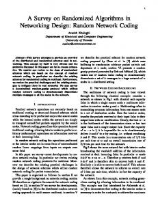
Figure 3.1 is an example that illustrates the conditions in Theorem 3.2. In this examc c ple, m = 7 and i = 6. The set of common parents is P67 = {v1 , v2 , v3 }. Hence, P(P67 )= c {Ø, {v1 }, {v2 }, {v3 }, {v1 , v2 }, {v1 , v3 }, {v2 , v3 }, {v1 , v2 , v3 }}. All the sets in P(P67 ) satisfy

the condition in Theorem 3.2 except v˜p = {v1 , v2 }, where mincut(S, {v6 } ∪ v˜p ) is equal to mincut({v6 } ∪ v˜p , v7 ) = 3. Malicious nodes vm with large number of incoming edges δI (vm ) are able to share a c greater number of parents with neighbor nodes. In other words, |P(Pim )|, the cardinality c of P(Pim ), is larger. Hence, it is more probable to find a v˜p that does not satisfy the

condition in Theorem 3.2. Such malicious nodes share null keys with neighbors and can conduct successful attacks with higher probability.


25

S !p ∪ vi 1

2

!p

vi

6

vm 7

3

4 !c 5

Figure 3.1: A network consisting of 8 nodes. The malicious node is v7 and the target node is v6 . However, if the condition in Theorem 3.2 is not satisfied, it does not imply that vm is capable of corrupting the content of node vi . For instance, a null key sent on a path, connecting vi and vm , does not increase the intersection between ΠKi and ΠKm once it is mixed with other random null keys. This random combination generates different values of null keys and guarantees an efficient protection against jamming attacks. The following theorem presents the conditions that apply on the paths crossing the minimum cut between vi and vm . Theorem 3.3 Consider a path p from vi to vm . Let v˜c be the set of nodes on the path p. If ∃ vc ∈ v˜c such that ΠKc * ΠKm , then the null key received on the path p does not increase the dimension of ΠKi ∩ ΠKm . Proof: Denote by K˜c the null keys matrix of v˜c . Since node vi sends a null key to v˜c on the path p, then dim(ΠKi ∩ ΠK˜c ) ≥ 1. Therefore, if ΠK˜c ⊆ ΠKm then dim(ΠKm ∩ ΠKi ) ≥ 1. On the other hand, applying Lemma 2 of [19], if ΠK˜c * ΠKm , then with high probability, the null key sent by v˜c to vm on the path p does not belong to ΠKi . Hence, the path p


26

does not contribute in increasing the dimension of ΠKi ∩ ΠKm , unless, ΠK˜c ⊆ ΠKm . This condition is satisfied if and only if ∀ vc ∈ v˜c , ΠKc ⊆ ΠKm .

t u

In the example shown in Figure 3.1, v˜c = {v5 }. The null keys received by v5 span a space ΠK5 * ΠK7 . Thus, the null key sent on the path (v5 , v6 ) does not increase the intersection space ΠK6 ∩ ΠK7 . Although there exists a v˜p = {v1 , v2 }, that does not satisfy the condition in Theorem 3.2, v7 fails to attack v6 . In fact, node v5 is adding randomness to the null keys communicated and hence contributing by increasing the immunity of neighbor nodes against jamming attacks. Let pc = Pr(ΠKc ⊆ ΠKm ). Then by Theorem 3.3, a null key sent on path p, connectY ing vi and vm , increases the dimension of ΠKi ∩ ΠKm with probability pc . This ∀ vc ∈v˜c

probability decreases as the number of nodes on the path p increases. This also applies to the paths connecting the parents of vi and node vm . In fact, under the conditions of Theorem 3.2, when the paths between v˜p and vm contain more nodes, it is less probable that ΠKi ⊆ ΠKm . Their subspace intersection decreases. Therefore, the corruption probability drops when the target node or the shared parents are far from the malicious node. This explains how our security scheme is able to limit the pollution in the network and isolate malicious nodes. Null Keys algorithm is more efficient in large scale networks. This is obvious, since the null keys go through a greater number of combinations when there are more participants. Thus, it is less probable that a malicious node shares null keys with neighbor nodes. The source provides immunity to the nodes by distributing null keys. Through random combinations a node generates new null keys and hide its content. The analysis shows that the pollution produced by a malicious node can be limited to a small area covering some of its neighbor nodes. Our security scheme is capable of isolating each malicious


27

node separately and limiting the pollution spread. In case the minimum cut between the source and a malicious node is equal or larger than the number of injected null keys, the source can distribute additional null keys to prevent this malicious node from jamming the network. For instance, only the source can transmit twice to its direct downstream nodes when distributing null keys. This is equivalent to doubling the out-degree of the source node. Hence, the minimum cut between the source and the nodes increases. Following the conditions of Theorem 3.2, Pr(ΠKi ⊆ ΠKm ) decreases. The only drawback in such scenario is that, the direct downstream nodes of the source have to validate the integrity of the null keys twice as many as in the previous scenario. Injecting additional null keys in the network increases the immunity of the nodes. On the other hand, if multiple malicious nodes {vm1 , vm2 , · · · } are allowed to exchange their null keys then they can be modeled as a single malicious S node, with an in-degree ΓI (vmi ). Hence, the same conditions and properties apply on this scenario. The efficiency of the attack from colluding malicious nodes depends on their total minimum cut to the source which defines the number of null keys they can collect.

3.3.3

Time Delay and Overhead

The distribution of null keys does not impose an initial delay on the system. In fact, the source does not wait until every node receives its null keys. Instead, it starts sending its blocks directly after injecting the null keys. As a node receives a new null key, it can clean its buffer if it contains corrupted blocks. As indicated in Section 3.2, the operations at the intermediate nodes remain unchanged. The same operations are performed on the null keys and on the data blocks.


28

In Null Keys algorithm, no redundancy is added to the source blocks. Adding extra bits to the data blocks can consume a significant capacity. For instance, in Charles et al. [10], the signature is transmitted together with the data. For a large file, these extra bits add up to become a substantial overhead cost to the system. On the other hand, although other methods that use homomorphic hashing do not add any overhead to the source blocks, they require heavy computations at intermediate nodes. This is the main drawback of such schemes which alter the network performance. In their paper [23], Krohn et al. showed that the expected per block cost of a hashing operation is ((r + d)λq /2 + r)M ultCost(p), where λq is a large random prime security parameter and M ultCost(p) is the cost of multiplication in the field of hash elements Zp . However, the Null Keys algorithm only requires a simple multiplication, which allows the nodes to perform fast data block verifications. The expected per block cost of the security check at a node v is c(r + q)M ultCost(q), where M ultCost(q) is the cost of multiplication in the field of arithmetic operations Zq and c is the minimum cut between v and the source. This computation cost can be derived from Equation (3.2). The cost can be further reduced when the verification process is done using one random combination of all received null keys. For example, in [23], the parameters λp and λq are equal to 1024 and 257 respectively. Therefore, the per block verification process at node v is around 771/c times faster than homomorphic hashing verification. The minimum cut c depends on the topology. For instance, in a random topology consisting of 1000 nodes with a connection probability of 1%, c is equal to 5 on average. Furthermore, the factor c can be reduced to one if the nodes use a random combination of all received null keys in the verification process. There is a trade-off between computation complexity and security performance. For

3.4. APPLICATION OF NULL KEYS IN REAL-WORLD TOPOLOGIES

29

instance, homomorphic hashing guarantees a high level of security since the hash functions are collision-free. However, due to the computation cost, security schemes that use homomorphic hashing require that nodes check blocks probabilistically. In our security scheme, we use homomorphic hashing to protect only the null keys. Node v performs δI (v) hash verifications instead of verifying all the r source blocks as in homomorphic hashing security. For example, the number of source blocks r is equal to 512 in [23] and [17]. On the other hand, if homomorphic hashing is used to verify the integrity of the data blocks, the information is delayed at each node. Such delay can drastically decrease the network performance. Hence, using homomorphic hashing to protect only the null keys intensely reduces the number of hashing verifications performed at each node and prevents the data blocks from being delayed in the network. Another drawback of hashing is the large field size that would be required. Limiting the use of homomorphic hashing operations preserves the network performance. Cooperative security is one approach that uses probabilistic checking. In Section 3.5, we compare the performance of Null Keys to cooperative security.

3.4

Application of Null Keys in Real-World Topologies

The performance of Null Keys algorithm depends on the subspaces intersection which in turn depends on the network topology. In this section we study the application of our security scheme in the topologies that model real-wold networks and internet topology. For instance, in the peer to peer file sharing Bittorrent [12], which dominates the


30

internet traffic, the peers randomly select their neighbors. On the other hand, Stutbach et al. [31] reported that Gnutella exhibits the clustering and short path length of small-world networks. Moreover, Faloutsos et al. [15] discovered that power-laws characterizes the topology of the internet at both inter-domain and router level. We show how the characteristics of each topology affects the performance of Null Keys algorithm with respect to providing immunity to network coding architectures against jamming attacks.

3.4.1

Random Topology

Random graphs have good robustness properties and are used by many file sharing peer to peer systems as Bittorrent [12] . The nodes randomly select their neighbors from the network. Each pair of nodes is connected with a probability p. The average degree of a node is approximately equal to np. Random topologies display a short global diameter. One of the main characteristics of random topologies is that on average, a short distance Lr separates any pair of nodes. Hence, it is more probable to find short distinct paths to the source and less probable to find v˜p satisfying the condition in Theorem 3.2. The nodes have similar in- and out-degree and contribute in efficiently communicating the null keys. This short distance allows the nodes to have access to different null keys and prevents malicious nodes from isolating them. In addition, the benefits of applying Null Keys in random networks is the large set of parent choices, independent of the distances or the degree distribution, available to the nodes. In fact, the condition in Theorem 3.2 is satisfied with high probability and the intersection of subspaces collected by neighbor nodes is minimal. The short distance and random parent selection contribute in hiding the value of null keys. Neighbor nodes collect null keys that span subspaces with minimum intersection. Hence for large scale networks,


31

nodes share a small number of parents and the subspaces intersection is minimal. The corruption of a node vi reduces to the case where the number of upstream malicious nodes limits the effectiveness of ΠKi . Hence, in large scale random networks, the corruption depends on the ration of malicious nodes to the network size. In such topologies, malicious nodes fail to isolate neighbors and to alter the communication of null keys. The randomness of the topology adds to the randomness of null keys generation and distribution which better hide the null keys content at the nodes. The unrevealed verification process effectively protects the nodes from excessive jamming attacks.

3.4.2

Small-World Topology

The topology of small-world networks, introduced by Watts and Strogatz [33], is a regular lattice, with a probability φ of short-cut connections between randomly-chosen pairs of vertices. In a small-world network, the average pairwise shortest path length Lsw is almost as small as that of a random graph Lr , while the clustering coefficient Csw is orders of magnitude larger than that of a random graph Cr . Studies have shown that large classes of networks are characterized by those properties. In fact, Stutzbach et al. [31] reported that Gnutella exhibit small-world properties. They showed that the graphs are highly clustered, yet they have short distances between arbitrary pairs of vertices. Furthermore, Wu et al. [35], discovered that streaming topologies evolve into clusters and exhibit small-world properties. A k-connected ring lattice is the base of the small-world model. All nodes in V are placed on a ring and are connected to neighbor nodes within distance k/2. We consider small-world with rewiring and small-world with shortcuts model. The rewiring model


32

is defined as follows. We go through the ring in a clockwise direction, considering each node in turn and with probability φ rewire each outgoing edge to a new node chosen uniformly at random from the lattice. Figure 3.2 shows the ring lattice we used to model small-world topology. If, instead of rewiring, we add an edge e we obtain the small-world with shortcuts model.

Figure 3.2: Directed ring lattice [2].

To study the performance of Null Keys algorithm in small-world networks, we consider the intersection of subspaces collected by the nodes vi ∈ V in their clustered neighborhood denoted as Ci . In a k-connected ring lattice, all the nodes in V have an in-degree and out-degree k. Costa et al. [13] showed that wiring does not alter the capacity of smallworld networks. They proved that, with high probability, the capacity of such model p falls within the interval [(1 − )k, k] where = 2(d + 2)ln(n)/k for a free parameter d. Hence, the graph is well connected and the nodes has access to k null keys. This is supposed to provide the nodes with an efficient resistance against malicious attacks. However, Watts et al. [33] showed that, as φ → 0, the separation between two nodes in the graph is Lsw ∼ n/2k and the clustering coefficient Csw ∼ 3/4. Hence, as φ → 0, the graph becomes highly structured and nodes highly separated, as a result, clusters share local information with common cuts to the source. Although node vi have access to k null keys, the intersection of subspaces spanned by the null keys collected in its clustered


neighborhood

T

vj ∈Ci

33

ΠKj ∼ k. If we consider the case where φ = 0, the source injects

null keys to its downstream nodes within a distance k/2. In any cluster Ci distant from the source, nodes are susceptible to jamming attacks in the presence of a single malicious node in Ci . In such scenario, for a malicious node vm , mincut(vm , vi ) = mincut(vi , S) for vm ∈ Ci , thus vm conducts successful attacks on vi . For increasing values of φ, Watts et al. [33] demonstrated that Lsw decreases immediately, whereas Csw remains significant. They showed that there is a broad interval of φ where Lsw ≈ Lr ∼ ln(n)/ln(k), whereas Csw Cr ∼ k/n. This intense decrease in the distance introduced by the rewired edges produce small-world networks. Those short cuts contract the distances between the clusters and the source. With a probability φδO (vi ), node vi connects to a random node in the graph which brings in information from distant nodes on the ring lattice and decreases the subspace intersection collected by the clustered neighborhood. As a result, the number of shared parents of vi and vm , on distinct paths, decreases and the probability that vm conducts successful attacks drops. The source edges are also rewired which allows a more efficient spread of null keys in the network and introduces distinct cuts to the source nodes. As φ → 1, Lsw ≈ Lr and Csw ≈ Cw and the performance of small-world networks converges to the performance of random networks.

3.4.3

Power-Law Topology

Power-law topology has been observed in router, inter-domain and world-wide-web topologies [15, 6, 4]. The graph metrics follow the distribution y ∝ xα which reflects the existence of a few nodes with very high degree and many with low degree. Figure 3.3 illustrates the degree distribution in power-law graphs.


34

Figure 3.3: Power-law graph. To study the application of Null Keys algorithm in power-law networks, we adopt the model proposed by Bollob´as et al. in [7]. This model describes undirected graphs by treating both in-degrees and out-degrees. It is simple and flexible. By manipulating several parameters, the model generates many different power-law graphs. The in- and out-degrees can be varied by changing the values of the parameters. In particular, the parameter β, which is the probability of adding an edge from two existing vertices according to their in- and out-degrees, varies the overall average degree. Also, parameters δin and δout control how steeply the degree frequency curve drops off, with smaller values indicating steeper curve. In our model, the in- and out-degrees of vertices grow at similar power-law rates, i.e., vertices with high in-degree have high out-degree. Denote by H the set of nodes hi with high in-degree δi (hi ) and out-degree δo (hi ), often called “Hubs”. Following power-law distribution, |H| |V |. Having a high indegree, vertex hi acts as a source of null keys to its downstream nodes, thus contributing in their security against jamming attacks. Chung et al. [11] showed that a power-law topology has the smallest characteristic path length log log n compared to random and


35

small-world topologies. Hence, for any vi ∈ V \H there exist, with high probability, a short path to a vertex hi ∈ H that does not contain malicious nodes. In other words, there exist a cut between vi and hi that does not intersect with paths from a malicious node vm to hi . As long as this short path exists, vi is immune to jamming attacks. Our attack model is similar to the attack defined in [5]. Albert et al. reported that scale-free networks are robust under random attacks. They argue that the robustness is due to the in-homogeneous connectivity distribution. In case the malicious nodes are selected randomly, with high probability vm ∈ / H, thus have small connectivity. Such nodes fail to attack neighbor nodes that are provided with null keys on the paths to the source or to hi ∈ H. Among the three models discussed, the distribution of null keys is faster and more efficient in power-law networks. However, if the malicious nodes are not randomly chosen, but instead are selected from H, the network becomes vulnerable to jamming attacks. Nodes hi ∈ H, which effectively contribute in protecting the network, can drastically jam it. For instance, if a low degree node vi is connected to a malicious node vm ∈ H then with high probability the paths between vi and S contain vm and ΠKi ⊂ ΠKm . In power-law distribution, such low degree nodes are frequent and susceptible to jamming attacks. The analysis is similar to [5], where the removal of high-degree nodes drastically decreases the ability of the remaining nodes to communicate with each other. In fact, when highly connected nodes are malicious, the communication of null keys decreases and the network becomes vulnerable to attacks. In Section 3.5, through simulations, we evaluate the performance of Null Keys in Power-Law model under attack of randomly selected and highly connected malicious nodes.

3.5. SIMULATIONS

3.5

36

Simulations

We evaluate the performance of Null Keys through simulations in the topologies discussed in Section 3.4. We use the percentage of corrupted nodes as a metric to measure the efficiency of the security schemes with respect to protecting network coding architectures from jamming attacks. We model the networks using the topologies discussed in Section 3.4. The block size is set to 128. We use directed graphs with a single source node. The malicious nodes are randomly selected from the network. They conduct smart attacks, as defined in Section 3.3, where they take advantage of the information they have access to. The simulator is round-based, where in each round a node can upload and download blocks. Each round, the attackers send one bogus block on each of their outgoing links trying to jam their neighbors. All the results presented in this chapter are averaged over several runs, specified by each scenario. We also use traces from a commercial peer-to-peer live streaming system UUSee [1] to study the performance of our security scheme in real-world systems. The topologies are obtained using snapshots from UUSee traces. We simulate and present the results of the performance of Null Keys algorithm in those live streaming systems. Finally, we compare with cooperative security introduced by Gkantsidis et al. [17] who show that cooperation guarantees better efficiency than other probabilistic approaches that use homomorphic hashing.

3.5.1

Performance in Real-World Models

First, we evaluate our security scheme in random models by connecting each pair of nodes with a probability p. We randomly choose a set of nodes to be malicious. As discussed in Section 3.4.1, the performance of null keys in random topologies depends on the

3.5. SIMULATIONS

37

connection probability p. A highly connected network guarantees a better communication

Percentage of Corrupted Nodes (%)

of null keys and hence, provides a greater protection against jamming attacks.

30 25 20

p=1% p = 0.8 % p = 0.5 %

15 10 5 0 0

200

400

Number of Malicious Nodes

600

Figure 3.4: Percentage of corrupted nodes as a function of the percentage of malicious nodes in a random network of 1000 nodes. In Figure 3.4, we show the pollution spread as a function of the percentage of malicious nodes. The network size is set to 1000 nodes and the results are averaged over 50 runs. We first note that as the percentage of attackers increases the corruption expands. The result is obvious since the connection to malicious nodes grows. Thus, the immunity of the nodes against jamming attacks decreases since malicious nodes do not provide neighbors with null keys that help detect bogus blocks. A greater number of malicious neighbor nodes can alter the access to null keys and hence, increase the susceptibility to jamming attacks. We also note that larger connection probabilities p result in a significant decrease in the percentage of corrupted nodes. The network is better connected for greater values of p. Thus, the nodes gain access to a larger set of null keys that helps in detecting bogus blocks. In fact, each node connects to a larger set of neighbors and the number

3.5. SIMULATIONS

38

of parents increases. Therefore, the source injects additional null keys which go through a greater number of linear combinations. In a highly connected network, the nodes contribute by increasing the randomness of the null keys and the attackers fail to alter their communication. The subspaces intersection, collected at the nodes, decreases and the malicious nodes capabilities become limited. In Section 3.3.3, we mentioned that the source node starts distributing its blocks directly after injecting the null keys. As a result, the nodes progressively receive null keys. Hence, the number of corrupted nodes varies as the participants collect their null keys. Any node can clean its buffer from bogus content as it receives a new null key. In Figure 3.5, we show how the corruption varies over the rounds of simulation in a network consisting of 1000 nodes. We observe that the pollution peaks at the initial rounds since there are few null keys available at the nodes. The curve descends as the nodes are cleaning their buffers usingg null keys recently received. We also observe that the corruption stabilizes at a low level where malicious nodes are isolated. For a connection probability p equal to 0.7% the corruption level reached is lower than that of p equal to 0.5%. This is due to the fact that a better connected network provides stronger immunity against jamming attacks when Null Keys algorithm is applied. The figure shows that our security scheme is able to drive the network to a stable state, where the number of corrupted nodes is fixed, which helps in isolating and locating the malicious nodes. Figure 3.6 provides a snapshot that captures the state of the nodes in a network size equal to 250. The corruption shown is at a stable state after the distribution of null keys. We can clearly observe that the effects of malicious nodes are restricted in the network, and the corruption spread is limited to small areas. This stable state of the nodes helps

Percentage of Corrupted Nodes

3.5. SIMULATIONS

39

20

Nm = 25 % Nm = 30 % Nm = 35 %

15 10 5 0 0

50

Round

100

150


(a) p = 0.5%

60

Nm = 25 % Nm = 30 % Nm = 35 %

50 40 30 20 10 0 0

50

Round

100

150

(b) p = 0.7%

Figure 3.5: Percentage of corrupted nodes variation over rounds in a network consisting of 1000 nodes. Nm refers to the percentage of malicious nodes.

3.5. SIMULATIONS

40

Malicious Uncorrupted Corrupted Source

Figure 3.6: A snapshot that captures the state of a network consisting of 250 nodes. in isolating malicious nodes in the network. In Figure 3.7, we show the effect of the network size on the pollution spread. The results are average over 30 runs. As indicated in Section 3.4.1, the percentage of corrupted nodes decreases as the network grows. In fact, in a large random topology a node has a greater number of neighbors choices to connect to, hence a smaller number of paths and parents shared with others. The subspaces intersection is smaller and the nodes are better protected. This explains the decrease in corruption when then network size is less than 400 nodes. However, for larger networks, the subspaces intersection factor becomes minimal and dominated by the case where most of upstream nodes are malicious which limits the access to null keys. Hence, the corruption depends on the percentage of malicious nodes. This is shown in Figure 3.7 for networks containing more than 500 nodes where the corruption converges to a stable level for fixed percentage of malicious nodes.


3.5. SIMULATIONS

41

7

Nm = 20 % Nm = 25 % Nm = 30 %

6 5 4 3 2 1 0

200

400 600 Network Size

800

1000

Figure 3.7: The effect of the network size on the pollution spread. Nm refers to the percentage of malicious nodes. Next, we study the security efficiency of Null Keys algorithm in small-world networks consisting of 1000 nodes as modeled in Section 3.4.2. Similarly, the attackers are selected randomly from the nodes in the network. We consider the parameters k, the rewiring probability φ that characterizes small-world networks and the percentage of malicious nodes in our simulations. We report the percentage of corrupted nodes as a metric to evaluate the efficiency of our security scheme. We show in Figure 3.8, the pollution spread as a function of the rewiring probability φ and the percentage of malicious nodes Nm . The results are averaged over 30 runs and the parameter k is fixed to 15. For small values of φ, the corruption can be significant. In fact, when the nodes are greatly clustered, the intersection of subspaces collected inside a cluster is high. Therefore, a malicious node is capable of polluting neighbors in its cluster. On the other hand, we see that a slight increase in the value of φ notably reduces the percentage of corrupted nodes. As depicted in Section 3.4.2, an increase in the value of


3.5. SIMULATIONS

42

50

Nm = 15 % Nm = 20 % Nm = 25 % Nm = 30%

40 30 20 10 0 0.1

0.2

0.3

Rewiring Probability

0.4

Figure 3.8: Percentage of corrupted nodes as a function of the rewiring probability φ in a small-world network of 1000 nodes. k is set to 15. φ results in an immediate reduction of the average distance Lsw , whereas the clustering coefficient, Csw , slightly decreases. Hence, the paths to the source become shorter and the subspaces intersection within the clustered nodes decreases. The null keys propagate more effectively for greater values of φ and provide better protection against malicious attacks. Moreover, observe that even when 30% of the nodes are malicious, Null Keys algorithm is capable of limiting the pollution spread and isolating the malicious nodes for increasing values of φ. Figure 3.9 shows the percentage of corrupted nodes in a network size equal to 1000, as a function of the parameter k. We randomly select 15% of the nodes to be malicious. The rewiring probability φ is set to 0.1. As indicated in Section 3.4.2, in small-world networks, the capacity of a k-connected ring lattice is around k with high probability. Thus, as we increase the value of k, nodes get access to a greater number of null keys. In addition, with a fixed rewiring probability, nodes connect to a greater number of neighbors


3.5. SIMULATIONS

43

100

Rewiring Adding

80 60 40 20 0

4

8

15

k

25 30

40

Figure 3.9: Percentage of corrupted nodes as a function of k in a small-world network of 1000 nodes. φ is set to 0.1 and 15% of the nodes are malicious. outside their clusters. As shown in the figure, this results in a significant reduction of the pollution spread. In fact, the intersection of subspaces collected by neighbor nodes decreases. Note the steep drop in the percentage of corrupted nodes when the parameter k is increased. However, for φ equal to 0, modifying the value of k does not change the vulnerability of the network since the nodes do not connect to neighbors outside their clusters. We also observe from Figure 3.9 that adding shortcuts instead of rewiring does not affect the percentage of corrupted nodes independent of the value of the parameter k. Although adding shortcuts instead of rewiring increases the minimum cut between the nodes and the source, it does not significantly change the intersection of subspaces collected in neighbored clusters. Hence, it does not change the immunity of the nodes against jamming attacks. The simulations show that for careful selection of the parameters φ and k, Null Keys algorithm can intensely reduce the pollution spread in the network. In fact, for increasing

3.5. SIMULATIONS

44

values of the rewiring probability φ, the average path length Lsw in small-world networks approaches that of random networks, Lr , allowing more random neighbor selections and hence effectively hiding the null keys content. The high clustering coefficient on the other hand, provides a robust node connectivity. Our security scheme proved to contain and isolate an excessive percentage of malicious nodes in a network modeled using small-world topology. Finally, we simulate our security scheme in power-law topology that also models realworld networks. The results are averaged over 30 runs in a network consisting of 1000 nodes. We study the security efficiency of Null Keys algorithm under two scenarios. First, we randomly select the malicious nodes from the network and report the percentage of nodes corrupted. Then, we select the malicious nodes from the set of high-degree nodes H and study the immunity of the network against jamming attacks. This set of nodes, defined in Section 3.4.3, characterizes power-law topology and plays an important role in the communication of null keys. Figure 3.10 shows the performance of Null Keys when the malicious nodes are randomly selected from the set of nodes V . We observe that our security scheme is resilient to jamming attacks from a high percentage of malicious nodes. In fact, in power-law networks, the high-degree nodes h ∈ H act as sources of null keys since they have access to a large set of null keys and provide them to downstream nodes. They guarantee and effective communication of null keys. Also, the average distance between any pair of nodes is smaller than that of random or small-world networks. Thus any node is closely connected to some h ∈ H and hence is protected from jamming attacks. The malicious nodes, randomly selected from a power-law graph, are low-degree nodes with high probability. Indeed, the set of high-degree nodes H is small compared to the set V . Hence,

3.5. SIMULATIONS


40 30

45

β = 0.5 β = 0.6

20 10 0

10 20 30 40 Percentage of Malicious Nodes

Figure 3.10: Percentage of corrupted nodes as a function of the percentage of malicious nodes in a power-law network of 1000 nodes. when randomly selected, the malicious nodes have very limited jamming potential. Furthermore, we observe that an increase in the value of β reduces the corruption spread. In fact, the network connectivity increases for larger values of β, hence nodes get access to a greater number of null keys. As previously stated, the subspaces intersection collected by neighbor nodes decreases when the network is better connected. On the other hand, if the selection of malicious nodes targets the high-degree nodes h ∈ H, the communication of null keys decreases as discussed in Section 3.4.3. In Figure 3.11, we show how the pollution expands as we select more nodes from the set H to be malicious. The percentage of malicious nodes is fixed to 30%, however we vary the percentage of the nodes in H that are malicious. Since such nodes can alter the nodes connectivity, they are capable of corrupting the content of neighbor nodes if they are malicious. However, we can see from the figure that our security scheme can contain the attack conducted by malicious nodes in H. For instance, when 60% of the nodes in H


3.5. SIMULATIONS

60

46

Nm = 30 %

50 40 30 20 10

20 40 60 80 Percentage of Malicious Nodes in H

Figure 3.11: Percentage of corrupted nodes evaluate by selecting different percentages of nodes in H as malicious. The power-law network consists of 1000 nodes and the percentage of malicious nodes is set to 30%. are malicious, only 30% of the nodes are corrupted. The remaining nodes are connected to a safe high-degree node h ∈ H which provides them with immunity against jamming attacks. However, in power-law networks, the high-degree nodes in H are usually trusted nodes. They can play an important role in securing the network as in our security approach. Such nodes contribute to the security of the network by effectively distributing the null keys received from the source. For any node, a single connection to any h ∈ H is sufficient to protect it from jamming attacks. The randomly selected malicious nodes have a minimal impact on the connectedness of the network while targeted malicious nodes in H can harm the node connectivity. Hence, only when the selection of malicious nodes targets the set H, the jamming attacks can damage the network. On the other hand, those high-degree nodes are very useful to protect the network and play an essential

3.5. SIMULATIONS

47

role in Null Keys security scheme.

3.5.2

Performance in UUSee-Like Model

We next investigate how Null Keys algorithm performs in real live peer-to-peer systems. For this purpose, we obtained snapshots of traces collected from UUSee Inc. [1] that reveal the topology of the network. UUSee is a live peer-to-peer streaming provider in mainland china that broadcasts over 800 channels to millions of peers. From the traces, we can determine the list of neighbors of each node which infers the topology. In our simulations, we used two snapshots from the measurements of peers in the UUSee streaming overlay to model the connections between the nodes. The first one consists of 2003 nodes and the second one consists of 5251 nodes taken at 14:51:58 and 19:02:26 respectively, on August 08, 2008. We apply our security algorithm on the inferred UUSee


topology and simulate malicious attacks on the nodes.

15 N = 2003 N = 5251 10

5

0 0

10 20 30 40 Percentage of Malicious Nodes

50

Figure 3.12: Performance of Null Keys algorithm in a network modeled using two snapshots from UUSee Inc. traces.

3.5. SIMULATIONS

48

Similarly, to evaluate the performance of our algorithm, we measure the percentage of corrupted nodes in function of the percentage of malicious nodes present in the network. From Figure 3.12, we observe that Null Keys is able to effectively contain the jamming attacks from a high percentage of malicious nodes. Also note that the nodes were able to limit the propagation of bogus blocks in both networks, modeled using the snapshots, with a slight difference in the damage produced. In fact, in UUSee protocol the nodes randomly select their neighbors from which they request media blocks as in random topologies. Furthermore, as discovered in [35, 36], the topology evolves into clusters inside each ISP as in small-world models. Hence, the same conditions of random and small-world topologies apply to UUSee topologies. The UUSee network represents a low network diameter which allows a fast and efficient distribution of null keys. The network is highly connected which prevents attackers from isolating the nodes and limiting the access to null keys. Indeed, in the UUSee streaming protocol, the nodes are highly connected since they establish connections and exchange blocks with around 30 nodes. Hence, the nodes participating in the UUSee live peer-to-peer session cooperate effectively in protecting the network when Null Keys algorithm is applied.

3.5.3

Performance Comparison

Finally, we compare Null Keys algorithm to another security scheme for network coding that uses homomorphic hashing. The hash verification presented by Krohn et al. in [23] guarantees a high level of security since it is collision-free. However, as show in Section 3.3.3, homomorphic hashes require heavy computations and cryptographic overhead. Our verification process, shown in Equation (3.2), can be around seven hundred times faster than the hash verification. Since homomorphic hashes are computationally expensive,

3.5. SIMULATIONS

49

they require that nodes check blocks probabilistically as in cooperative security, proposed by Gkantsidis et al.[17]. In their model, Gkantsidis et al. use homomorphic hashing to check for malicious blocks. The nodes perform probabilistic verifications in order to reduce the computation cost imposed by homomorphic hashes. In order not to weaken the verification process, they proposed that nodes cooperate in checking for malicious blocks. Whenever a node detects the presence of bogus blocks, it sends alert messages to neighbor nodes. To compare both security approaches, we implemented the cooperative security scheme. We assume, as in [17], instantaneous propagation of alert messages. A node checks blocks with probability pc . Once a malicious block is detected, all the infected nodes are informed. A node sends alert messages to the upstream nodes that have sent unsecured blocks, and downstream nodes that have received unsecured blocks. In our model, the graph is directed, however we assume that alert messages can propagate to upstream nodes. In Figure 3.13, we show the percentage of corrupted nodes achieved in both Null Keys and cooperative security schemes in the same network model as a function of the percentage of malicious nodes. We used a random topology consisting of 1000 nodes where the connection probability p is set to 0.5%. We clearly see that Null Keys algorithm guarantees a better protection than cooperative security against jamming attacks. Under the attack of the same percentage of malicious nodes, our security scheme limits the pollution spread better than cooperative security, even for a checking probability of 40%. As pc increases the percentage of corrupted nodes decreases, but the computation costs augment. Note that when the percentage of malicious nodes is greater than 20%, the slow increase in the corruption can be explained by the overlap in the affected regions. In


3.5. SIMULATIONS

40

30

50

Pc=1% Pc=5% Pc=20% Pc=40% NK

20

10

0

10

20

30

Percentage of Malicious Nodes

40

Figure 3.13: Comparison between Null Keys and cooperative security performances in a random network of 1000 node with p = 0.5%. NK refers to Null Keys and pc refers to the probabilistic checking in cooperative security. fact, when the polluted regions overlap, the same block can be corrupted multiple times. Hence, all overlapping attacks can be discovered once this block is detected. Another drawback of cooperative security is that a node stops using unsecured blocks when an alert message is received which alters the network performance since non-corrupted blocks can be part of theses unsecured blocks. The cleaning process is slow since homomorphic hashing is used. On the other hand, Null Keys algorithm uses a fast verification to check the integrity of the data blocks and hence does not impose any significant delay on their propagation. In addition, the edge connection probability p does not change the results in the case of cooperative security, as claimed in [17]. However, for larger values of p, our security approach can perform even better as shown in Figure 3.4. Indeed, in the comparison, the edge connection probability is set to 0.5%, which is the worst case in Figure 3.4.

3.5. SIMULATIONS

51

Also, in the case of cooperative security, the corruption is dynamic. In contrast with our approach, the corruption state of the nodes always varies. Depending on which nodes perform the verification check and how the alert messages propagate, the corruption of the nodes varies. Hence, the locations of malicious nodes cannot be approximated. However, Null Keys algorithm proved to drive the network to a stable corruption state with a limited damage.

Chapter 4 Progressive Encoding for Network Diagnosis In this Chapter, we present a trace collection protocol that utilizes progressive encoding to disseminate peers vital statistics, referred to as snapshots, in the network. We focus on the scalability of the protocol and its resilience to high level of peer dynamics. The peers cooperate by allocating cache capacity for snapshots generated by other peers. Our results show that the server is able to decode most of the snapshots generated under large-scale peer departures.

4.1

Motivation and Objective

In this part of the thesis, we seek to solve the problem of monitoring large-scale peerto-peer systems using a trace collection protocol that allows the server to gather measurements from the participating peers. The main requirement is to collect most of the traces from a highly dynamic large-scale peer-to-peer system. The traditional solution 52

4.1. MOTIVATION AND OBJECTIVE

53

involves sending periodic reports to a centralized server, as in UUSee [1]. Those periodic snapshots represent a large traffic volume that can shut down the server. Due to the limited server bandwidth, the traces should be disseminated in the network first and then, collected by the server in a delayed fashion, in order to gather snapshots from the peers that have already left the session. To tolerate snapshot losses due to peer dynamics, some redundancy should be injected in the network. In order to increase data diversity and to be resilient to losses and failures, network coding is applied to disseminate the traces such that only coded blocks are exchanged and stored in the network. The main advantage of using network coding is to increase the diversity of the data blocks to effectively disseminate the traces in the network. Instead of introducing redundant blocks in the network, the peers exchange coded blocks to resist peer departures. These coded blocks are used to reconstruct the traces even after the departure of the sources. We believe, however, that the challenge is to find a practical way of using network coding for live trace generation. The key factor is the segment size that allows the protocol to scale and tolerate peer dynamics. A segment is a group of blocks on which random linear codes are applied. If we choose a segment size equal to the number of participating peers, we would limit the scalability of the protocol. In fact, the coded blocks would contain all the original blocks generated during an epoch and thus their sizes grow with the network size. On the other hand, if we reduce the segment size to the number of blocks generated by a single peer during an epoch, we would limit the blocks diversity. Note that the peers cannot wait for a long period of time before encoding their data, since their traces would be lost at the time they depart. In order to allow our protocol to scale and, at the same time, increase the diversity of the exchanged blocks, we propose to use progressive encoding to disseminate the traces. Our protocol adapts

4.2. PROTOCOL OVERVIEW

54

to peer dynamics and controls the redundancy introduced in the network. Therefore, it allows the coded blocks to effectively spread in the network to tolerate heavy peer departures.

4.2

Protocol Overview

We present a new trace collection protocol for large scale live peer-to-peer applications. The protocol allows continuous trace generation from peers and continuous trace collection by the server. Depending on their Quality of Service experience, the peers generate vital statistics and exchange them with neighbors allowing the participating peers to cache them in a decentralized fashion. We do not assume a periodic fixed size trace exchange but rather the peers produce data independently at any time depending on their Quality of Service experience. Such trace generation allows the peers to produce more traces when experiencing important performance changes and to disseminate them even at the time they have to leave the session. On the other hand, the server allocates a small bandwidth to periodically pull data from a randomly selected set of peers during the streaming session. By buffering the traces in the network, we prevent the peers from uploading their data simultaneously and hence we allow the server to collect excessive data traffic in a delayed fashion when the number of peers increases dramatically. In order to be tolerant to peer dynamics, the trace collection mechanism disseminates copies of the data generated in the network. By introducing redundancy in the network, the server can pull the traces produced by the peers even after they have left the session. In our protocol, we use randomized linear network coding for traces exchange and storage. Network coding increases the diversity of the data blocks and the tolerance to block losses upon peer departures. Network coding is performed within segments,

4.2. PROTOCOL OVERVIEW

55

where each segment is defined by each peer as the set of blocks forming their snapshots. Random linear combinations are applied to each segment, i.e. to the blocks generated by the same peer. For instance, a peer that has received blocks, that belong to the same segment generated by the same peer, sends random linear combinations of those blocks to neighbors and stores one coded block to be sent to the server when probed. The segment size is a key factor in the design of the trace collection protocol. The best solution would require maximizing the segment size. As such, we maximize the blocks diversity and solve the caching capacity problem of the peers. When the segment size is small, the snapshots are less tolerant to peer dynamics and the peers inject more segment in the network. Therefore, neighbors would have to decide which segment to cache and which segment to send. In contrast, when the segment size is larger, the coded blocks can be better disseminated in the network without generating many dependencies. The goal is to propagate the coded blocks to as many peers as possible, in order to resist peer departures, without resulting in many block dependencies at the server. In our protocol, we apply random linear codes on segments defined as the groups of original blocks produced at each peer. We propose to use progressive encoding to increase the diversity of the blocks in the live trace generation. Hence, the segment size grows as a peer produces new data blocks. The peers perform progressive encoding by grouping newly generated traces in a segment containing previous traces already disseminated in the network. Hence, the segment size is defined by each peer and increases depending on the Quality of Service experience. As the segment size increases, the blocks are disseminated further in the network to tolerate peer departures. Hence, peers control the redundancy introduced in the network by modifying the segment size. A cached block is replaced with its random linear combination with a newly received block that belongs

4.3. TRACE COLLECTION PROTOCOL

56

to the same segment and which can contain more coefficients. Through progressive encoding, the peers effectively disseminate the coded blocks in the network. Also, the protocol takes advantage of the fact that the server is periodically probing the network since blocks containing different number of coefficients are utilized to reconstruct the snapshots and hence, are used to decode parts of the segment they belong to. Finally, our protocol adapts to peer dynamics by allowing the peers to adjust the amount of disseminated coded blocks depending on their local view of neighbors’ departure rate. We study and present an in-depth view of our protocol in the subsequent sections.

4.3

Trace Collection Protocol

In this section, we present our trace collection protocol which applies progressive random linear network coding on the snapshots disseminated in the network. We assume that all the peers allocate a cache capacity to store snapshots from other peers. The participating peers encode blocks that belong to the same segment, hence generated by the same peer. They generate and distribute snapshots independently without any time interval restrictions. We first present the data block format and then describe our trace collection protocol.

4.3.1

Data Block Format

The format of the coded data block addresses the progressive encoding used in our trace collection protocol. Figure 4.1 shows the format of the data block. We include the ID of the peer that produced the trace associated with the data block. We also include an entry to indicate the segment number defined by the peer that has produced the block.


57

The SF entry represents the spreading factor that defines how far should the blocks associated with this segment propagate. We append the coefficients used in the encoding process and the payload that represents the coded data block. ID

Seg

SF

C1

C2

...

Cs

Payload

Figure 4.1: Data block format. The peers do not exchange any acknowledgements or requests, instead they only disseminate sufficient data blocks in the network so that the server can decode their traces. The server, on the other hand, does not send any acknowledgment to the peers, instead it pulls a fixed amount of data Qs from the network every period of time Ts and reconstructs original segments when possible. Otherwise, such messages would lead to significant overhead when used.

4.3.2

Protocol Description

Our goal is to control the redundancy introduced by the dissemination of the traces in the network and to efficiently store the coded blocks in the peers’ caches until they are collected by the server. We start by discussing the spreading factor entry, shown in Figure 4.1, that corresponds to the group of blocks forming a segment k. Its value is set by the peer that has generated the segment and is modified whenever new blocks are added to the segment. The spreading factor determines the number of blocks that should be disseminated in the network. In other words, it is an indicator of the number of peers that should be reserving an entry in their caches for that segment k. In our trace collection protocol, the spreading factor of a segment depends on its size, defined by the number of blocks it contains, and the neighbors’ departure rate. In fact, coded


58

blocks belonging to a larger segment should be cached more frequently in the network for the server to decode them. Furthermore, a higher spreading factor guarantees better tolerance to peer dynamics. Blocks should spread further in the network to resist losses due to high level of peer departures. In our protocol, peers can choose the appropriate spreading factor for the newly generated data blocks based on the local view of neighbor dynamics. Hence, the number of coded blocks disseminated in the network adapts to the dynamic of the peers. The spreading factor of a segment k is calculated using a logarithmic function as shown in Equation (4.1). We use a logarithmic function to take into account previously disseminated blocks of segment k. Those blocks, with different number of coefficients, are used in the decoding process by the server. The spreading factor is defined as

SF = α(d) log2 (βnc + 1),

(4.1)

where nc is the number of coefficients of segment k. The parameters α(d) and β determine the redundancy or the number of coded blocks to be injected in the network. The variable d is the dynamic percentage rate measured using the local view of neighbor dynamics. It is the rate at which the neighbors leave the session. In our protocol, α(d) is a step function as shown in Equation (4.2). A peer measures its neighbor dynamics and modifies the spreading factor based on its sensitivity indicated by the departure percentage levels pl .


   α1 d p l l

59

(4.2)

Our design objective is to effectively cache the traces in the network and communicate them in a manner that could resist the high level of peer dynamics and allow the server to reconstruct the traces by periodically pulling a fixed amount of arbitrarily blocks from the network. The protocol is implemented using progressive encoding as shown in Algorithm 4.3.2. Upon experiencing Quality of Service changes, a peer produces new measurements to be collected by the server. Consequently, it generates traces and divides them into blocks of size 1 KB each which fits in a single UDP packet. Then, it adds those blocks to its segment k that was previously disseminated in the network. After modifying the segment and increasing its size, the peer recalculates the spreading factor SF using Equation (4.1). Accordingly, when it decides to inject those newly generated blocks in the network, it sends coded blocks from segment k. A peer can decide to switch to a new segment when nc reaches a maximum value that leads to significant coefficient overhead. Note that the blocks exchanged in the network, that belong to the same segment, can have different number of coefficients. Such blocks are encoded together after appending a corresponding number of zeros to adjust their sizes. Upon receiving new data blocks from a segment k, a peer retrieves the spreading factor from the messages. It then applies random linear combinations to the newly received blocks and the cached blocks that belong to that same segment k. According to the retrieved spreading factor, it sends coded blocks to neighbor peers and sets their


Algorithm 2 Trace Collection Protocol. Sending original coded blocks M ← collect measurements b ← divide M and packetize it into block of 1KB each B k ← previously disseminated segment or new segment ID bk ← B bk ∪ B b B bk ) + 1) SF = α(d) log2 (β × sizeof (B for u = 1 to sizeof (N eighbors) P SFu ← Randomly distribute blocks s.t. SFu = SF for i = 1 to SFu bk ) random coefficients from GF (2q ) C ← sizeof (B bk b=C ×B Send b to peer u end for end for Receiving coded blocks b ← received coded blocks B SF ← retrieved message spreading factor SF = SF − 1 ID ← retrieved message source ID k ← retrieved message segment ID j ← Cache entry for segment k from peer ID b0 ← B bj ∪ B b B for u = 1 to sizeof (N eighbors) P SFu ← Randomly distribute blocks s.t. SFu = SF for i = 1 to SFu b 0 ) random coefficients from GF (2q ) C ← sizeof (B b0 b=C ×B Send b to peer u end for end for b 0 ) random coefficients from GF (2q ) C ← sizeof (B if j == Ø if cache is full j ← oldest cache entry else j ← new cache entry end if end if bj = C × B b0 B

60

4.4. PERFORMANCE ANALYSIS

61

appropriate SF entries. Finally, it stores a coded block by replacing previous cache entry of the segment k, if it exists. In case the cache is full, it replaces the oldest segment entry in the cache memory. Hence, as the segment size increases, the blocks propagate further in the network replacing previous versions of that same segment. The number of disseminated coded blocks is determined by the spreading factor set by the peer that has produced the measurements. Progressive encoding is significant and effective when we avoid using acknowledgments and requests in the trace collection protocol. In fact, through the segment replacement mechanism, progressive encoding solves the problem of data block caching, where the peers have to decide wether to keep an existing block or replace it with a new one. The idea behind using progressive encoding is to increase blocks diversity in order to spread traces to as many peers as possible without introducing many block dependencies at the server. By encoding previously disseminated blocks with newly generated blocks, we increase blocks diversity in live trace generation. The server, on the other hand, collects blocks belonging to segments that are increasing in size as it periodically probes the network and deletes them from the peers’ caches. With progressive encoding, such cached blocks are more meaningful since they help decoding segments that are increasingly containing newly generated blocks. In addition, we avoid the problem of decoding all or nothing since the server can decode part of the segment if it has collected enough blocks during its periodic probing.

4.4

Performance Analysis

In this section, we study the overhead generated by the dissemination of coded blocks and the relationship between the parameters of our trace collection protocol discussed in


62

the previous sections.

4.4.1

Data Dissemination Overhead

In order for the design to scale, it should control the redundancy introduced by the dissemination of the snapshots in the network. The segment size is an important factor in regulating the overhead involved in our trace collection mechanism. With progressive encoding, the coefficient overhead of a segment depends on its size defined by the number of coefficients nc it contains. Network coding operations are performed over a Galois field 2q . In a network of n peers the coefficient overhead is around r × q + log2 n bits. We limit the size of a block to 1KB which fits in a single UDP packet. On the other hand, the communication overhead is defined by the redundancy ratio and the cache capacity allocated by the peers. Redundant blocks are not duplicates distributed in the network. Instead, when network coding is applied, redundant blocks are additional coded blocks exchanged. The server has to collect nc blocks in order to decode a segment containing nc coefficients. However, to tolerate peer dynamics, peers have to disseminate additional blocks which introduces redundancy in the network. Based on the protocol described in Algorithm 4.3.2, the redundancy ratio is defined as

RR =

α(d) log2 (βnc + 1) . nc

(4.3)

Note from Equation (4.3) that the redundancy adapts to the dynamics of the peers. Based on the local view of neighbor dynamics, a peer can adjust the spreading factor of its segments. Indeed, with higher level of peer dynamics, a peer should disseminate more blocks to tolerate the loss due to the departure of neighbors storing its data. Hence our


63

trace collection protocol adapts to peer dynamics and prevents redundant blocks from flooding the network. As previously discussed, the cooperation of the peers is determined by the cache capacity allocated to store blocks from other peers. Peers with long lifetime contribute the most to the system. In our design, we fix the cache capacity allocated for other peers and replace oldest entries when the cache is full. Peers store one copy of each segment received, to be sent to the server once probed. Each block pulled from the network is deleted from the caches.

4.4.2

Decoding Condition

In order to simplify the analysis, we assume that the events occur at discrete time t = 0, T, 2T, . . . . Consider a peer that has generated a segment k of size nc and has disseminated its coded blocks to C peers in a network of size N . The server has to collect nc coded blocks in order to decode and reconstruct the snapshots. However, the server uses a limited bandwidth to periodically probe the network consisting of dynamic peers that leave the session at a constant rate. We assume that the session terminates when all the peers depart. Table 4.1: Trace Collection Protocol Parameters Number of participating peers at time t Nt Number of peers storing blocks from segment k at time t Ct Redundancy ration RR Server probing rate Rp Peers’ departure rate Rd Number of collected blocks at probing time t xt

We use the parameters, shown in Table 4.1, in our analysis. We denote by Ct the


64

number of peers that store coded blocks from segment k at time t. Also, we denote the number of participating peers at time t by Nt . Assume that the server probes the network at a rate of one coded block from each of Rp peers every period of time T . The peers, on the other hand, depart at rate Rd peers every period of time T . Hence, in this scenario, we have Nt = N − t × Rd and the redundancy ration RR = C/nc . Assume that the random variables Ct at different times t are independent. We define Ct as the number of peers that have cached blocks from segment k after the departure of t × Rd peers. The probability P (Ct = l) is equivalent to the probability that C − l peers that store coded blocks from segment k have left the session before time t. We thus have

P (Ct = l) =

C C−l

N −C tRd −C+l N tRd

.

(4.4)

The expected value of the random variable Ct is

E(Ct ) =

min{C,N −tRd }

1 N tRd

X l=0

C l C −l

N −C . tRd − C + l

(4.5)

Define the random variable xt as the number of collected blocks by the server when it probes the network at time t. The variable xt follows a binomial distribution with parameters Rp and

Ct . Nt

The probability that the server collects l coded blocks from

segment k at time t by probing l peers storing those blocks is P (xt = l) =

Rp l

Ct Nt

l

Ct 1− Nt

Therefore, the expected value of xt is E(xt ) = Rp ×

Ct . Nt

Rp −l .

(4.6)

In other words, the expected

number of collected coded blocks when the server probes the network at time t is equal


to Rp × N , Rd

t=

Ct . Nt

65

Since the session terminates when all the peers leave the session at time

we express the total number of collected blocks as the random variable X such

that N/Rd

X=

X

N/Rd

x t = Rp

t=0

X Ct . N t t=0

We thus have N/Rd

E(X) = Rp

X E(Ct ) t=0

Nt

N/Rd

X E(Ct ) N − tRd t=0   N/Rd min{C,N −tRd } X 1 Rp X  C N −C . l N C − l tR − C + l N − tR d d tR t=0 l=0

= Rp

=

d

In order for the server to reconstruct the snapshots from segment k, it has to collect at least nc independent coded blocks. Hence, the expected number of collected blocks E(X) should be at least equal to nc . Therefore, we need to enforce the following condition: N/Rd

Rp N tRd



X 

t=0

1 N − tRd

min{C,N −tRd }

X l=0

l

C C −l



N −C  ≥ nc . tRd − C + l

(4.7)

In our trace collection, the parameter C in condition (4.7) can be replaced by RR ×nc which refers to the number of coded blocks disseminated in the network, hence, the number of peers that store a coded block from segment k. It is evident that a larger segment size nc requires more peers to store coded blocks. Note that the further the right hand side of condition (4.7) exceeds the segment size, the higher is the expected number of dependent blocks at the server. In our protocol, we approximate the rates and messaging intensity in order to satisfy condition (4.7).

4.5. PROTOCOL EVALUATION

66

We note from condition (4.7) that the most efficient way to disseminate the coded blocks is by spreading the blocks to as many peers as possible. In fact, increasing the number of coded blocks stored at the peers does not adjust the value of C to satisfy condition (4.7). Instead, C only depends on the number of peers storing coded blocks from segment k. By choosing the appropriate messaging intensity we satisfy the condition and hence tolerate the peer dynamics. This also applies to the number of segments generated by a single peer. To better resist network dynamics, a peer should maximize the segment size used and hence, minimize the number of injected segments to efficiently spread its coded blocks in the network. For this purpose, we implement progressive encoding in our trace collection protocol, through which, we increase the segment size and control the redundancy introduced in the network.

4.5

Protocol Evaluation

In this section we study the efficiency of our trace collection protocol and its resilience to high level of peer dynamics. We simulate a live peer-to-peer session where the peers continuously exchange data blocks as previously discussed in order to disseminate their snapshots in the network. The duration of the session is 600 minutes. We use eventdriven simulations and model the peer dynamics using exponential distribution with a mean value e. The peers generate traces and send their blocks independently. We also model their behavior using exponential distribution. The mean of the distribution ai defines the aggressiveness of a peer i. The server collects a fixed amount of data Qs from the network every period of time Ts . The number of blocks generated by the peers during the session should be less than Qs × Ts in order for the server to decode all the traces. We use the ratio of decoded blocks to the blocks generated as a metric to evaluate


67

our protocol under different level of peer dynamics. We also measure the redundancy collected or the linear dependent blocks collected by the server. Furthermore, we evaluate the messaging intensity defined as the average number of blocks sent by each peer during the session. We generate various random topologies and investigate parameters such as peer dynamics, associated with the mean of the exponential distribution e, the peers’ cache capacity and the spreading factor SF . In the simulations, we fix the parameter β of SF to 0.25 and vary α(d).

4.5.1

Delayed Data Collection

Through simulations, we show how our protocol can scale to large-scale peer-to-peer networks. For this purpose, we report the percentage of generated blocks decoded by the server when it periodically pulls a fixed amount of data from the network. With this delayed trace collection, the server can handle large-scale peer-to-peer networks and prevent peers from sending simultaneous excessive data. Figure 4.2 shows the number of decoded blocks in function of the spreading factor in a network consisting of 1000 peers. We fix β to 0.25 and vary the parameter α(d) of the spreading factor SF . In this scenario α(d) does not depend on the neighbor dynamics. We model the peer dynamics by setting the mean of the exponential distribution e to 100 minutes. We notice that the peers generate around 30,000 blocks during the session. The server collects a fixed amount of 800 blocks every 10 minutes. By caching the coded blocks in the peer-to-peer network, the server is able to collect and reconstruct the traces under the specified rate of peer departures. We notice from Figure 4.2, that for small values of SF , the redundancy created in the network is not sufficient to tolerate the peer dynamics which limits the decoding capabilities of the server. On the other hand, as we


68

increase the spreading factor, the blocks reach more peers and hence resist losses due to peer departures. Therefore, the server is able to collect enough packets to reconstruct most of the traces generated. We also observe that the number of dependent blocks collected by the server slightly increases. In fact, the redundancy disseminated in the network are coded blocks that are equally useful in the decoding process and progressive encoding increases the diversity of the blocks exchanged. This is one of the advantages of using progressive network coding for blocks dissemination. Moreover, we note that the message intensity is around 900 KB. It increases as we increase the spreading factor. In fact, more redundancy is cached in the network and more data blocks are exchanged by the peers for larger values of α(d).

4

4

x 10

Number of blocks

3 Generated Decoded Dependent Message Intensity

2 1 0

20

40

α(d)

60

80

Figure 4.2: Message intensity and decoding efficiency as a function of the spreading factor. α(d) is the variable and β is set to 0.25. Furthermore, to clearly see how the server collects data in a delayed fashion, we report the blocks dissemination and collection in function of time in Figure 4.3. Note that the


69

number of blocks collected follows a straight line since the server periodically pulls 800 blocks from the network, and as such prevents the peers from uploading excessive flows. The gap between the curves demonstrates how the blocks are disseminated first in the network and then collected by the server at a later time. Between time 150 and 400 the blocks generation slows down since the number of participating peers dramatically decreases. The remaining peers, with a long lifetime, store the snapshots of other peers that have already left. We observe from Figure 4.3, how the server is able to pull data from those peers until time 400, where all the participants have left the session. Note that in this scenario, the server was able to reconstruct more than 90% of the generated snapshots. The difference between the number of blocks collected and those disseminated, shown after 400 minutes, is equal to the number of dependent coded blocks collected by server. 4

4

x 10

Number of blocks

Disseminated Collected 3

2

1

0 0

200

Minutes

400

600

Figure 4.3: Blocks dissemination and collection in function of time. In Figure 4.4, we show how the probing quantity Qs affects the decoding efficiency.


70

We fix the probing period Ts to 10 minutes. The parameter α(d) and β of the spreading factor are fixed to 50 and 0.25 respectively. Also the network size is set to 1000. Figure 4.4 reveals that the decoding is limited when the number of collected blocks is less than the number of generated blocks. We note a fast increase in the amount of decoded packets as the Qs × Ts approaches the number of blocks generated by the peers. A probing quantity Qs equal to 800 is sufficient to allow the server reconstruct most of the traces. As we further increase Qs , the number of decoded packets slightly increases but the amount of linear dependent blocks collected by the server increases significantly. Hence, a careful selection of probing quantity Qs , can save the server bandwidth from dependent coded blocks. 4

4

x 10

Number of blocks

Generated

Decoded

Dependent

3

2

1

0

500

1000 Q

1500

s

Figure 4.4: Probing efficiency as a function of the periodic probing quantity Qs . Figure 4.5 demonstrates how the progressive encoding used in our trace collection protocol allows the server to reconstruct some snapshots from a segment received, even when it does not have enough blocks to decode all the segment. We report the number


71

of decoded blocks collected from a randomly selected peer u, as the server is periodically probing the network. Figure 4.5(a) shows the distribution of the collected blocks from peer u as a function of the number of coefficients retrieved from the messages. On the other hand, Figure 4.5(b) shows how the number of decoded blocks increases as the server collects additional data. For instance, we observe that although the server collected 7 blocks containing 10 coefficients each, it was able to decode them using previously collected blocks containing only 5 coefficients. All the blocks reported in Figure 4.5 belong to the same segment. The server was able to decode 60 out of the 80 blocks forming the segment. Figure 4.5 shows that our protocol increases the diversity of the exchanged blocks through progressive encoding and allows the server to reconstruct snapshots from a segment without the need to completely decode it. Indeed, when Algorithm 4.3.2 is applied during a session, the segments sizes grow and the number of coefficients contained in the exchanged blocks increases. As the server periodically pulls data form the network, blocks containing different number of coefficients are used in the decoding process. As such, we avoid the problem of decoding all the segment or nothing. Next, we fix the probing quantity Qs to 800 and the probing period Ts to 10 minutes and investigate the effect of the peers’ cache size on the protocol. We set the mean value of the exponential distribution that models peer dynamics to 80 minutes. Figure 4.6 shows that with a cache size of 100 KB the amount of decoded blocks is limited to 60% independent of the spreading factor. In fact, the peers that have a longer lifetime are supposed to cache the data blocks of the peers that have left the session in order for the server to pull their blocks in a delayed fashion. However, with a cache size of 100 KB the peers have to drop blocks previously buffered. The server fails to collect sufficient number of blocks to reconstruct additional snapshots under such rate of peer


72

30

Received blocks

25 20 15 10 5 0 0

20

40 60 Coefficients

80

(a)

Decoded blocks

60 50 40 30 20 10 0 0

20

40 60 80 Received blocks

100

(b)

Figure 4.5: Reconstructing blocks of a segment collected by the server.


73

departures. We also observe that a cache size of 300 KB is sufficient to allow the server decode most of the blocks generated using an appropriate spreading factor. We note a slight decrease in the decoding efficiency for small cache sizes. This is due to the fact that for large values of α(d), segments occupy peer caches more than needed by the server, creating additional dependency and preventing other generated blocks from getting buffered. In our protocol, progressive encoding decreases the number of segments injected in the network and through segment replacement mechanism it efficiently uses the neighbors’ cache capacity.

Percentage of decoded blocks

100 90

Cache = 400 Cache = 300 Cache = 200 Cache = 100

80 70 60 50 40

20

40

α(d)

60

80

Figure 4.6: The effect of cache size on the decoding efficiency.

4.5.2

Peer Dynamics Factor

Our trace collection protocol adapts to peer dynamics and controls the redundancy disseminated in the network. We study the effect of peer dynamics and show how our protocol can tolerate high level of peer departures. By modifying the spreading factor


74

SF , based on their local view of neighbor dynamics, peers can determine the redundancy that should be disseminated in the network. In order to reveal the relation between the spreading factor and the peer dynamics, we evaluate the percentage of decoded blocks under different values of the parameter e, as shown in Figure 4.7. The network size is set to 3000 peers. We note that under extreme level of peer dynamics, where e is equal to 30 minutes, the spreading factor parameter α(d) is required to be as high as 90 in order for the server to reconstruct most of the traces. With such rate of peer departures, the cached blocks losses prevent the server from reconstructing the generated snapshots. Hence, a segment should spread further in the network reaching more peers in order to tolerate such high level of peer dynamics. However, selecting a large value for α(d) under a low peer departures rate would result in many block dependencies at the server. Therefore, the spreading factor should be chosen according to the peer dynamics. In our protocol, peers determine the number of blocks to disseminate using Equation (4.1) which is a function of neighbors’ dynamic percentage rate. In the previous scenarios, the parameter α(d) did not depend on neighbor dynamics d. However, Figure 4.7 indicates that the peers should modify the spreading factor depending on the rate of peers’ departure. Since a peer does not have a global knowledge of peer dynamics, it modifies its spreading factor based on the local view of neighbor dynamics. In our protocol, as the rate of neighbor departures augments, a peer increases the spreading factor of its segment to disseminate additional coded blocks in the network. As the blocks are disseminated further in the network, a peer can tolerate neighbor dynamics and hence allow the server to collect its data and reconstruct its snapshots. The redundancy ratio RR of Equation (4.3) is an indicator of the level of redundancy


75

Percentage of decoded blocks

100 80 60 e = 120 e = 100 e = 50 e = 30

40 20

20

40

α(d)

60

80

Figure 4.7: Decoding efficiency as a function of the spreading factor under different level of peer dynamics. Network consists of 3000 peers. injected in the network. In our simulations, we calculate RR by measuring the ratio of blocks disseminated in the network to blocks generated by the peers. We report in our results the percentage

1 RR

where smaller values of

1 RR

imply higher redundancy exchanged

by the peers. In the scenario of Figure 4.8, α(d) has a single sensitivity level p1 at which the peers change their spreading factor according to Equation (4.8). The parameter β of SF is set to 0.25 and the peers vary α(d) depending on their neighbor departures rate. We fix the mean value e of the exponential distribution, that models peer dynamics, to 20 minutes.    50 d p  1

(4.8)

We observe from Figure 4.8 that for small values of p1 , the server is able to reconstruct more snapshots. Indeed, when the peers are more sensitive to neighbor departures,


76

80

Percentage

60

40

Decoded blocks 1/RR

20

0 0

20

40 60 p1 Level

80

100

Figure 4.8: Decoding efficiency and message intensity as a function of the dynamic sensitivity level. they adjust their spreading factor faster and hence resist high level of peer dynamics by injecting additional coded blocks in the network. On the other hand, for large values of p1 , many coded blocks would be lost before the peers decide to adjust the spreading factor used. Note that when we reduce the sensitivity level p1 , the redundancy ratio increases. In fact, when p1 is small, more peers would increase their spreading factor and hence increase the messaging intensity. Peers become more sensitive to their neighbor dynamics and more blocks are exchanged and cached in the network. Finally, we fix the sensitivity levels and vary the mean value e to study how our trace collection protocol adapts to high level of peer dynamics. For this purpose, we apply our protocol in a network consisting of 5000 peers under different levels of peer departures. Peers change the spreading factor they use according to Equation (4.9) and thus, adjust the messaging intensity.


100

77

Decoded blocks

1/RR

Percentage

80 60 40 20 0 0

20

40

e

60

80

100

Figure 4.9: Protocol’s adaptability to peer dynamics in a network consisting of 5000 peers. The variable e is the mean of the peer dynamics distribution model.

   30 d

on the application of random linear network coding for ... - TSpace

on the application of random linear network coding for ... - TSpace

Suggest Documents

on the application of random linear network coding for ... - TSpace

Random Linear Network Coding: A free cipher?

Implementation of Random Linear Network Coding on OpenGL ...

Implementation of Random Linear Network Coding on OpenGL

Random Linear Network Coding For Time Division ... - Semantic Scholar

Random Linear Network Coding for Time-Division ... - Semantic Scholar

Random Network Coding

The Capacity of Random Linear Coding Networks

Throughput-Delay Analysis of Random Linear Network Coding ... - arXiv

Implementation of Random Linear Network Coding using NVIDIA's ...

On Random Network Coding Based Information Dissemination

Bounds on the Network Coding Capacity for Wireless Random ... - arXiv

Random Linear Network Coding: A free cipher? - CiteSeerX

On Linear Network Coding - Google Sites

Optimized Random Network Coding for Reliable

On Linear Network Coding - Google Sites

On error control codes for random network coding - Semantic Scholar

On error control codes for random network coding - CiteSeerX

Decoding Algorithms for Random Linear Network Codes

The Efficiencies of Decoding Methods in Random Network Coding for ...

Broadcasting XORs: On the Application of Network Coding in Access ...

Construction of Error-Correcting Codes for Random Network Coding

On Fractional Linear Network Coding Solution of Multiple

Linear Network Coding on Multi-Mesh of Trees