on the comparative performance of bayesian and classical ... - CiteSeerX

Sankhy¯ a : The Indian Journal of Statistics 2002, Volume 64 Series B, Pt. 3, pp 239-266

ON THE COMPARATIVE PERFORMANCE OF BAYESIAN AND CLASSICAL POINT ESTIMATORS UNDER ASYMMETRIC LOSS By D. BHATTACHARYA Visva-Bharati University, India, F.J. SAMANEIGO University of California, Davis, USA and E.M. VESTRUP DePaul University, Chicago, USA SUMMARY. A comparison between Bayes and classical estimators was executed by Samaniego and Reneau (1994) in a univariate context involving exponential families, conjugate priors and squared error loss. In that study, the Bayes risk with respect to a hypothesized true distribution on the unknown parameter was taken as the criterion by which estimators were evaluated, with the (possibly degenerate) true prior serving as a representation of the true state of nature. The main outcome of that work was the identification of the threshold separating the class of priors available to the statistician into those that outperform the best classical estimator from those that do not. It was found that, in general, Bayes rules outperformed classical rules unless the operational prior used was poorly centered and also placed a substantial amount of weight on the prior mean. These results were extended to higher dimensions by Vestrup and Samaniego (2002). There are, of course, many applications in which the assumption of symmetric loss is untenable. In the present work, a comparative analysis is executed when the loss function is asymmetric. More specifically, the performance of Bayes and classical point estimators, as measured by the Bayes risk relative to a fixed true prior distribution, is assessed when the loss function is the LINEX (linear exponential) loss criterion introduced by Varian (1975). We examine a variety of parametric paradigms, and also investigate a univariate estimation problem which arises in a regression framework. We obtain a number of analytical results pertaining to special cases in which the operational prior is “mean-correct” (that is, has the same mean as the true prior) or is highly diffuse. In general, both of these circumstances tend to favour the Bayesian approach. Paper received July 2001; revised May 2002. AMS (2000) subject classification. Primary 62F10, 62F15. Keywords and phrases. LINEX loss, Bayes estimator, multivariate normal, linear regression, Poisson, mean-correct priors, maximum likelihood.

240

d. bhattacharya, f.j. samaniego and e.m. vestrup

1.

Introduction

The problem of point estimation of a location parameter in one or several dimensions is most often treated as a symmetric problem in which positive and negative estimation errors of the same magnitude are considered to be of equal seriousness. Thus, average squared error or absolute error, or their natural multivariate generalizations, tend to be the loss criteria of choice in decision theoretic treatments of estimation problems. This assumed symmetry has served to compromise the practical utility of some of these results. Indeed, in applications in which the consequences of overestimation (for example) are considered to be much more severe than those associated with underestimation, the superiority of one estimator over another under squared error loss is really quite irrelevant. Various authors have postulated viable formulations of asymmetric loss criteria and have studied the comparative performance of two or more competing estimators under such loss structures. The present paper is dedicated to an examination of this type, applying analyses of the sort introduced by Samaniego and Reneau (1994) to asymmetric problems. Specifically, we will examine the comparative performance of certain classes of Bayes estimators with certain classical (or “frequentist”) competitors in problems in which a particular type of asymmetric loss criterion is deemed to be tenable. Before discussing the problems to be treated in more detail, we will describe the context in which problems of this type arise, and will review some of the relevant literature. ˆ represents the loss to the statistician when he/she estimates the If L(θ, θ) ˆ then we might be interested in a loss function parameter θ by the value θ, having the property L(θ, θ + c) > L(θ, θ − c) for any constant c > 0. Varian (1974) introduced the LINEX (linear exponential) loss function, given in its most general form by




ˆ = b exp[a(θˆ − θ)] − c(θˆ − θ) − d , L(θ, θ) where a and c are nonzero constants and b and d are positive. For this loss function to have certain desirable characteristics, the constants a, b, c, and d must be subjected to further constraints. In order for the loss to be equal to zero when θˆ = θ, that is, when there is no estimation error, we will wish to have d = 1. In order for L to be minimized when θˆ = θ, we require that a = c. Since the constant b is simply a scale factor that’s common to each of the three terms, we may, without loss of generality, set b = 1, yielding the more common form of the LINEX loss function used in univariate estimation

Bayesian and classical estimators under asymmetric loss

problems:



241



ˆ = exp a(θˆ − θ) − a(θˆ − θ) − 1. L(θ, θ)

(1)

It is easy to verify that the function L(∆) = exp [a∆] − a∆ − 1, where ∆ represents θˆ − θ, (1) is a convex function of ∆ on the real line, (2) is decreasing for ∆ ∈ (−∞, 0) and (3) is an increasing function for ∆ ∈ (0, ∞). When the constant a is positive, L grows exponentially in positive ∆, but behaves approximately linearly for negative values of ∆. Thus, when a > 0, LINEX loss imposes a substantial penalty for overestimation. We will restrict attention to positive a in this paper, but note that the treatment of negative a, the case in which the greater penalty attaches to underestimation, is completely analogous. Varian (1975) motivated the use of the LINEX loss function on the basis of an example in which there was a natural imbalance in the economic results of estimation errors of the same magnitude. He argued that LINEX loss was a rational way to formulate the consequences of estimation errors in real estate assessment. Other applications in which the need for asymmetric loss functions has been noted include problems in hydrology, reliability engineering and pharmaceutics. The estimation of peak water level in the construction of dams or levies is a problem in which overestimation represents a conservative error which increases construction costs, while underestimation corresponds to the much more serious error in which overflows might lead to huge damages in the adjacent communities. In engineering contexts, it is often the case that the overestimation of system reliability can result in a higher level of risk of unanticipated and catastrophic failures, one would prefer to err on the conservative side in such problems. In the health sciences arena, overestimating the safety risk of a drug may lead to more restricted use of the product, and thus reduced sales, while the underestimation of the safety risk would tend to encourage overuse of the product, with potentially disastrous and costlier consequences. For more detail on these and other examples of the natural occurrence of asymmetric loss, see Zellner and Geisel (1968), Aitchison and Dunsmore (1975), Zellner (1986), Kuo and Dey (1990), Basu and Ebrahimi (1991), Shao and Chow (1991), Pandey, Singh and Mishra (1996), Thompson and Basu (1996), and Huang and Liang (1997). As suggested by Varian’s work (1975), the derivation of the Bayes estimator of a parameter of interest will often be quite straightforward under LINEX loss. Indeed, it is easy to show that the Bayes estimator of θ with respect to the prior distribution G on θ under LINEX loss can be expressed

242

d. bhattacharya, f.j. samaniego and e.m. vestrup

(when it exists) as 1 θˆ = − log {E[exp(−aθ)]} , a where the expectation is with respect to the posterior distribution of Θ, given X = x . As we will see, the derivation of measures of performance of these and other estimators, for example, the Bayes risk of an estimator relative to a hypothesized “true prior” different from G, is also often expressible in closed form. In the comparisons to be made in the sequel, we will wish to discuss the circumstances in which a Bayes estimator of a given parameter relative to a fixed “operational” prior G outperforms the classical (frequentist) estimator of that parameter under LINEX loss. The present work extends the ideas and results in Samaniego and Reneau (1994) and Vestrup and Samaniego (2002) to the asymmetric case. Following these authors, we adopt, as the performance criterion in the comparison, the Bayes risk of a given estimator θˆ relative to the “true prior” G0 , a possibly degenerate probability distribution representing the true state of nature of the unknown parameter θ; the Bayes risk of interest is given by ˆ = EΘ EX|Θ L(Θ, θ), ˆ r(G0 , θ)

(2)

where Θ ∼ G0 . This criterion seeks to compare the performance of two estimators relative to the hypothesized “truth” G0 . From such comparisons, the general characteristics of prior distributions that perform well relative to classical estimators can be identified, and guidance regarding “good prior modelling” can be gleaned. For a more extensive discussion of the Bayes risk criterion in this type of problem, see Samaniego and Reneau (1994). In the sections that follow, we treat the comparison of Bayes estimators with the standard classical estimator in several different parametric paradigms. In Section 2, we treat the problem of estimating the mean of a k-variate normal population, k ≥ 1 (with diagonal covariance matrix), using the multicomponent version of LINEX loss proposed by Zellner (1986), that is, with ˆ = L(θ, θ)

k 

L(θi , θˆi ).

i=1

In that problem, we show that a Bayes rule with respect to a mean correct conjugate prior (that is, a conjugate prior G for which EG Θ = EG0 Θ) dominates the sample mean provided the level of dispersion in G is not too great. This result extends Theorem 1 of Samaniego and Reneau (1994) to the normal problem with asymmetric loss. It is also shown that a Bayes rule

Bayesian and classical estimators under asymmetric loss

243

with respect to a conjugate prior G with arbitrary mean will outperform the sample mean when the prior is sufficiently diffuse. Additional numerical and graphical studies are carried out with a view toward describing areas of Bayesian superiority under other conditions (i.e., fixed prior bias and diffusion). These are discussed in the concluding section. In Section 3, we treat the univariate problem of estimating a linear combination of parameters in a general linear model, again finding that Bayes rules with respect to mean-correct priors, as well as Bayes rules with respect to sufficiently diffuse priors, dominate the standard estimator of the parameter of interest. In the final section, our theoretical findings are illustrated via a reanalysis of the baseball batting average data of Efron and Morris (1975), and general guidance is offered regarding the choice of an estimator in problems involving asymmetric loss. Comparisons for Poisson data appear in the appendix. 2.

Estimating the Mean of a Normal Distribution with LINEX Loss

In this section, we pursue the comparison of Bayes estimators of a normal mean with the classical estimator, the sample mean, under LINEX loss, using Bayes risk relative to a hypothesized true prior as the performance criterion. In seeking conditions under which one estimator dominates the other, two sets of circumstances are of particular interest. The first is the comparison of the two estimators when the operational prior is quite diffuse. It was shown by Samaniego and Reneau (1994) that, under squared error loss, Bayes rules tend to outperform classical estimators when the operational prior is sufficiently diffuse. Does this result generalize to nonsymmetric situations? A second question of interest concerns the relative performance of a Bayes estimator when the operational prior is mean-correct, that is, when G has a mean that is equal to the mean of G0 . Of particular interest is the case in which G0 is degenerate, corresponding to the case where the parameter θ is an unknown constant. It is possible to answer both of these questions affirmatively; the precise answers, applicable to the normal models of arbitrary dimension k, are provided in Theorems 1 and 2 below. When k is taken as 1, these results constitute direct analogs to problems considered by Samaniego and Reneau (1994) for squared error loss. In what follows, we compare Bayesian and frequentist estimates of the mean of a k-variate normal distribution via the Bayes risk with respect to a “true prior distribution” G0 . We first assume that 2 I]. X|Θ = θ ∼ Nk [θ, Σ = σ 2 I] and Θ ∼G Nk [θ G , ΣG = σG

(3)

244

d. bhattacharya, f.j. samaniego and e.m. vestrup

The true prior distribution will be modeled as 2 I]. Θ ∼G0 Nk [θ G0 , ΣG0 = σG 0

We use the multivariate extension of Varian’s LINEX loss function, which ˆ = (θˆ1 , · · · , θˆk ) of θ = (θ1 , · · · , θk ) is given by for an estimate θ ˆ = L(θ, θ)

k  



ˆ eai (θi −θi ) − ai (θˆi − θi ) − 1 .

(4)

i=1

The Bayes rule with respect to the operational prior G will again be denoted (1) (k) by dG = (dG , · · · , dG ), and it is easily verified that for i = 1, · · · , k, (i)

dG (x) = E(Θi |X = x) = −


 1 log E e−ai Θi , ai

(5)

where the expectation above is with respect to the posterior distribution of Θ|X = x relative to the operational prior G. To compute this posterior expectation, we observe that Θ|X = x



∼ Nk ΣG (ΣG + Σ)−1 x + Σ(ΣG + Σ)−1 θ G , ΣG − ΣG (ΣG + Σ)−1 ΣG



for arbitrary covariance matrices Σ, ΣG , and ΣG0 . Then, taking the specific forms of these covariance matrices into account, we obtain 

Θ|X = x ∼ Nk



2 2 σ2 σ2 σG σG x + θ , I . G 2 2 2 σG + σ 2 σG + σ 2 σG + σ 2

It follows that for each i, 

Θi |X = x ∼ N1



2 2 σ2 σ2 σG σG x + θ , i iG 2 + σ2 2 + σ2 2 + σ2 , σG σG σG

and hence we have for each i that


−ai Θi

E e





|X = x = exp −ai





2 2 σ2 σG σ2 a2i σG x + θ + 2 + σ2 i 2 + σ 2 iG 2 + σ2) σG σG 2(σG



.

Therefore, letting a = (a1 , · · · , ak ), we have that the Bayes rule with respect to the operational prior G and LINEX loss is dG (x) =

2 2 σ2 σG σ2 σG x + θ − G 2 + σ2 2 + σ2 2 + σ 2 ) a. σG σG 2(σG

(6)

Bayesian and classical estimators under asymmetric loss

245

We wish to compare r(G0 , dG ), the Bayes risk of dG with respect to the true prior, to r(G0 , dM L ), the Bayes risk of the maximum likelihood rule dM L with respect to the true prior, where dM L (x) = x. (In general, the MLE is ¯ , but we have without any loss of generality reduced the vector of means x this to the case of n = 1 by invoking sufficiency.) To do this, we must obtain the aforementioned Bayes risks. We calculate the former Bayes risk first, obtaining the risk function R(θ, ·) along the way. We have, letting E denote expectation with respect to X|Θ = θ: R(θ, dG ) =

k  








e−ai θi E eai (λ1 Xi +λ2 θiG −ai λ3 ) − ai (E {λ1 Xi +λ2 θiG −ai λ3 } −θi ) −1 ,

i=1

where λ1 =

2 2 σ2 σ2 σG σG = λ1 . , λ = 1 − λ , and λ = 2 1 3 2 + σ2 2 + σ2) 2 σG 2(σG

Utilizing the fact that λ1 Xi ∼ N1 [λ1 θi , λ21 σ 2 ], we have that




1

2 2 a2 i

E {λ1 Xi } = λ1 θi and E eai λ1 Xi = eai θi λ1 + 2 λ1 σ

.

Substitution of these quantities into the risk expression and some algebra yield that R(θ, dG ) equals k

 i=1



1 exp −ai λ2 θi + ai (λ2 θiG − ai λ3 ) + a2i λ21 σ12 2



+ai λ2 θi − ai (λ2 θiG − ai λ3 ) − 1 . We now take the expectation of this expression with respect to the true prior distribution G0 , and E will now denote expectation with respect to G0 . First, since 



1 2 E {Θi } = θiG0 and E {exp (−λ2 ai Θi )} = exp −λ2 ai θiG0 + λ22 a2i σG , 0 2 have that r(G0 , dG ) = E{R(Θ, dG )} may be expressed after substitution and algebra as r(G0 , dG ) =

k

 i=1





1 1 2 2 2 exp ti ∆i + t2i (σG − σG ) − ti ∆i + ai ti σG − 1 , (7) 0 2 2

246

d. bhattacharya, f.j. samaniego and e.m. vestrup

where for i = 1, · · · , k we have ∆i = θiG − θiG0 and ti =

ai σ 2 2 + σ2 . σG

(8)

Thus, having obtained the Bayes risk of dG relative to G0 , we now turn to the Bayes risk of dM L relative to G0 . It is shown in Zellner (1986) that R(θ, dM L ) =

k

 i=1





1 2 2 a σ −1 , exp 2 i

which shows that dM L is an equalizer rule relative to the parameter θ. Thus, it trivially follows that r(G0 , dM L ) =

k

 i=1





1 2 2 a σ −1 . exp 2 i

(9)

Now that the Bayes risk of both dG (7) and the MLE (9) have been specified, we compare the risk expressions. Theorem 1. For arbitrary values of the operational prior mean θ G and the true prior mean θ G0 , the Bayes risk of the Bayes rule dG is smaller than that of the maximum likelihood rule dM L if the operational prior is sufficiently diffuse. Proof. Letting θ G and θ G0 be arbitrary, observe that lim r(G0 , dG ) =

2 →∞ σG

k  a2i σ 2 i=1

2

and recall that r(G0 , dM L ) =

k  i=1





exp

a2i σ 2 2





−1 ,

2 . Utilizing the inequality x < exi − 1 (true for all real x ) with free of σG i i 2 2 xi = ai σ /2 for i = 1, · · · , k shows that

lim r(G0 , dG ) < r(G0 , dM L ),

2 →∞ σG

which means that for some threshold value V depending on the distance between θ G and θ G0 , the Bayes rule dG dominates the standard rule dM L 2 > V . This completes the proof. for all choices of σG

Bayesian and classical estimators under asymmetric loss

247

Theorem 2. Under the condition of mean-correctness (θ G = θ G0 ), the Bayes rule dG has smaller Bayes risk with respect to G0 than does dM L if 2 > σ 2 , that is, the Bayes rule dominates if the operational prior distriσG G0 bution is more diffuse than the true prior distribution. In particular, in the 2 = 0, the Bayes rule always classical point estimation framework where σG 0 dominates the MLE when the operational prior is mean correct. 2 > σ 2 , the Bayes Proof. Under the mean correct situation with σG G0 risk (7) becomes

r(G0 , dG ) = <
0, which means that we must show 

l ΣG − ΣG (ΣG + σ 2 (X  X)−1 )−1 ΣG



− σ 2 ΣG X  (XΣG X  + σ 2 I k )−2 XΣG l > 0. If we can show that Ψ = ΣG −ΣG (ΣG +σ 2 (X  X)−1 )−1 ΣG −σ 2 ΣG X  (XΣG X  +σ 2 I k )−2 XΣG is positive definite (a stronger result than what is needed), this subclaim will follow. Using the identities (17) and (18) for X  (XΣG X  + σ 2 I k )−1 and (XΣG X  + σ 2 I k )−1 X found in the proof of Theorem 3, we have that Ψ = ΣG − ΣG (ΣG + R)−1 ΣG − ΣG (ΣG + R)−1 R(ΣG + R)−1 ΣG , where R = σ 2 (X  X)−1 . Again, we simultaneously diagonalize the matrices R and ΣG by writing ΣG = ADA and R = AA , where A is invertible and D is a diagonal matrix with positive elements. Upon substitution and algebraic simplification, we obtain 



Ψ = AD D −1 − (D + I p )−1 − (D + I p )−2 DA. Since D −1 −(D+I p )−1 −(D+I p )−2 is easily verified to be a diagonal matrix with positive entries, it is positive definite. It follows that Ψ is positive definite. This proves subclaim (ii), and completes the proof of Theorem 4. 4.

Discussion

In this paper, we have studied several estimation problems with a view toward comparing the performance of Bayes and classical estimators under the LINEX loss criterion. We have used as a measure of performance the Bayes risk of each estimator relative to a hypothesized “true prior distribution” which represents the true state of nature. In the degenerate case, the latter situation models the unknown parameter as a fixed constant. In the problems studied here, we have given conditions under which Bayes estimators relative to mean-correct priors outperform the classical estimator [that is, the maximum likelihood estimator], and under which Bayes estimators

Bayesian and classical estimators under asymmetric loss

259

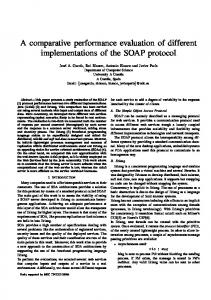
with respect to a prior which misspecifies the mean by a substantial amount will also outperform the MLE. These results effectively replicate the findings of Samaniego and Reneau (1994) and Vestrup and Samaniego (2002) under squared error loss. The general performance of Bayes estimators under LINEX loss in the univariate normal problem has also been investigated, albeit graphically rather than analytically. The findings there serve to confirm and extend our analytical results. Figure 1 below shows the graph of the set of level curves for the difference of the Bayes risks of the two estimators relative to a fixed “true prior” in the univariate version of the problem considered in Section 2. µ 14 a bc

d e f

12 g

10

8

6 2.0

3.5

5.0

6.5

σ2 8.0

Figure 1: Level curves of d = r(G0 , dG ) − r(G0 , dM L ) as functions of µG and σG . (a: 0.004385, b: 0.003594, c: 0.002803, d: 0.002013, e: 0.001222, f: 0.00043, g: –0.000360) The interior of the parabolic regions shown in this figure identifies the collection of mean-variance pairs of the operational priors for which the Bayes risk of the Bayes estimator is less than that of the MLE by at least that constant. Since the innermost level curve corresponds to a negative difference, the Bayes estimators relative to all operational priors with meanvariance pairs corresponding to that curve are better than the sample mean by the amount 0.00036. The mean and variance of the true prior used in the comparison in Figure 1 are 10 and 4 respectively with the parameter a of the LINEX loss function set equal to one. It is apparent that the Bayes rule

260

d. bhattacharya, f.j. samaniego and e.m. vestrup

dominates the MLE in this problem whenever the variance of the operational prior is sufficiently large, as guaranteed by Theorem 1. In conformance with Theorem 2, Bayes estimators with respect to mean-correct operational priors with variance greater than 4 are seen to outperform the MLE. Finally, the circumstances under which the MLE proves superior to the Bayes estimator are also shown in Figure 1. When the operational prior is not mean-correct and the operational prior variance is relatively small (reflecting a poor prior guess at the parameter and too much weight placed on the guess), the MLE outperforms the Bayes estimator. An especially interesting insight regarding asymmetry can be drawn from the curves in Figure 1. In spite of the fact that the LINEX loss function heavily penalizes overestimation, Bayes rules based on priors that overestimate the parameter perform only slightly worse than Bayes rules that underestimate the parameter by the same amount. Of course either of these estimators will outperform the MLE when the prior is sufficiently diffuse. As another illustration of our theoretical findings and the interpretations discussed above, we have carried out an actual comparison utilizing the famous batting average data set in Efron and Morris (1975). There, the batting averages for 18 players based on the first 45 at-bats in the 1970 season were given. Where Yi represented the batting average of player i in these first 45 at-bats in 1970 and pi represented the true batting average for the remainder of the season, Efron and Morris defined √ Xi ≡ 45 sin−1 (2Yi − 1), √ θi ≡ 45 sin−1 (2pi − 1), so that X|Θ = θ was N18 [θ, I]. Here the elements of θ denote the transformed batting average of each of the respective players over the rest of the 1970 season. Thus, the goal is to estimate the (transformed) batting average of each player for the rest of the 1970 baseball season (the θi ’s), based on each player’s average (transformed) from their first 45 at-bats (the Xi ’s) in the 1970 season. Since each player’s batting average became known at the end of the season, it is possible to calculate exactly the observed LINEX estimation ˆ = (θˆ1 , · · · , θˆ18 ) by error of each estimator, which is given for all estimators θ ˆ = L(θ G0 , θ)

18




ai exp(θˆi − θiG0 ) − ai (θˆi − θiG0 ) − 1 ,

(19)

i=1

where we will take a = 1, so that overestimation results in a steeper penalty than does underestimation.

Bayesian and classical estimators under asymmetric loss

261

We will compare the maximum likelihood estimator dM L (x) = x and 2 I] prior. G is the distrithe Bayes rule dG with respect to a N18 [θ G , σG 0 bution degenerate at θ G0 , where the elements of θ G0 are the true batting averages for the remainder of the 1970 season, transformed utilizing the formulas above. We will execute a comparison of dM L to dG for three possible prior means θ G : (a) θ G as the vector of transformed 1969 batting averages, (b) θ G as the 18-vector (−3.37, · · · , −3.37) , where -3.37 is the sample mean of the 18 xi values we are considering, and (c) θ G as the 18-vector (−2.04394, · · · , −2.04394) , which corresponds to a .350 batting average under the arcsine transformation used by Efron and Morris. We will denote (j) these three candidates for θ G by θ G , where j = 1, 2, 3 corresponding to situations (a), (b), and (c). When we use the maximum likelihood rule dM L , which estimates the batting average for the rest of the 1970 season based on the average of the first 45 at-bats for the 1970 season, the observed loss (19) by this rule becomes L(θ G0 , dM L (x)) = L(θ G0 , x) =

18 

{exp(xi − θ iG0 ) − (xi −θ iG0 )−1} = 9.282.

i=1

The components of the Bayes rule dG for any prior mean θ G and prior 2 are given by (6) with σ 2 = 1 and each element of a being one. variance σG A little algebra yields dG (x) =

2 (x − .5) + θ σG i iG . 2 +1 σG

2 and a prior mean θ For each choice of σG G the observed loss is therefore given by 18  i=1





2 (x − .5) + θ σG i iG − θiG0 exp 2 σG + 1





−

2 (x − .5) + θ σG i iG − θiG0 2 σG + 1





−1 ,

(20) and it is of interest to see how this number for the various choices of θ G 2 compares with the value 9.282 for the observed LINEX loss for the and σG maximum likelihood rule. 2, In Figures 2-4, the observed LINEX loss is plotted as a factor of σG the prior variance, for the prior distributions used in cases (a), (b), and (c) discussed above.

262

d. bhattacharya, f.j. samaniego and e.m. vestrup

Figure 2: Observed Linex loss when the prior mean is the vector of transformed 1969 Averages.

Figure 3: Observed Linex loss when the prior mean is the constant vector with components equal to the overall batting average of the eighteen players in their first 45 at bats in 1970. In summary of the above example, it is very hard for the Bayesian in this case to accrue a larger observed loss than the frequentist who uses the maximum likelihood rule. Even in cases where the Bayesian has a prior mean that overestimates the true value, only extreme dogmatism (a small 2 ) as to his prior guess will allow the frequentist rule to outperform the σG Bayes rule in the sense of observed LINEX loss. These results illustrate and confirm our theoretical findings in Section 2.

Bayesian and classical estimators under asymmetric loss

263

Figure 4: Observed Linex loss when the prior mean is the constant vector with components equal to a transformed batting average of .350. While we have focused all of our attention on the investigation of estimation problems based on the normal model, the range of problems to which these methods and ideas apply is quite a bit broader than this. Because of the particular form of the LINEX loss function, analytical comparisons of the sort we have pursued are feasible for any modelling framework in which the moment generating function of the posterior distribution exists in closed form. As an example of such extensions, we will develop in the appendix, the comparison of the Bayes estimator with the MLE in the case of Poisson-distributed data. An example of an exponential family that will resist analytical treatment of the comparison of interest is the family of Beta distributions. We conclude by mentioning that there are many other parametric paradigms that could be investigated via the type of program executed above. Clearly, analytical studies are quite feasible when posterior distributions take certain benign forms. In other cases, numerical investigations must suffice for gaining insight into the behaviour of competing estimators. The development of Bayesian inference for general, non-conjugate priors under LINEX loss, and the study of the comparative performance of the resulting estimators, will no doubt benefit from the recent renaissance in Bayesian computation. From the present study, we are inclined to conjecture that the domains of Bayesian superiority we have encountered – namely, the dominance of Bayes estimators with respect to either mean-correct or fairly diffuse priors – will surface again in other contexts. Our findings suggest that, even in non-symmetric situations, the Bayesian approach does two things: (i) it tends to benefit from careful calibration relative to the “truth” when such

264

d. bhattacharya, f.j. samaniego and e.m. vestrup

calibration is possible, and (ii) it tends to result in reasonable performance when the prior distribution is relatively diffuse, that is, when one understates rather than overstates one’s confidence in the prior mean. Appendix Assume that a random sample is available from a Poisson distribution with mean θ, that is, X1 , · · · , Xn are iid P (θ), the Poisson distribution with mean θ. We take the operational prior to be a member of the conjugate class of gamma priors Γ(α, β), where a member of this class has density function f (x|α, β) =

β α α−1 −βx x e (x > 0). Γ(α)

Thus, we take the operational and true prior distributions as G : Γ(αG , βG ) and G0 : Γ(αG0 , βG0 ). Since the posterior distribution of θ with respect to the operational prior G is also gamma, that is, 

θ|X = x ∼ Γ αG +

n 



xi , βG + n ,

i=1

one can easily derive the Bayes estimator with respect to G, namely 1 dG (x) = − α



αG +



n 

xi log

i=1

βG + n . βG + n + α

The Bayes risk of the estimator dG relative to the true prior G0 can then be derived as 

r(G0 , dG ) =

α 1+ βG + n 

+

αG +

 αG

nαG0 βG0

 



αG

1 1+

log

αβG βG0 (βG +n)

0



ααG0 βG + n + − 1. βG + n + α βG0

This is to be compared to the Bayes risk of dM L , which is given by 

r(G0 , dM L ) =

βG0

βG0   + α + n 1 − eα/n

αG

0

− 1.

Bayesian and classical estimators under asymmetric loss

265

While the two expressions above can be compared numerically without much difficulty, analytical comparisons are in general quite challenging. One particular case for which a definitive result can be obtained is the case in which the true prior G0 is degenerate and the operational prior G is relatively diffuse. To obtain the Bayes risks under these conditions, it is convenient to reparametrize the gamma in terms of the parameters λ and µ, where α = λµ and β = λ. We then can obtain a diffuse prior with mean µ by allowing λ to tend to zero, while a degenerate prior will result from allowing λ to tend to +∞. The two Bayes risks that result from taking such limits are given by 

2 σG

0

n lim r(G0 , dG ) = nµ log 2 n + α −→0 σG −→+∞

and





+ aµ



lim r(G0 , dM L ) = exp −µ n + α − neα/n



2 −→0 σG

.

0

Now since



nµ log

1 1+

 a n

+ aµ ≤

a2 µ , 2n

and since 



exp − n + α − ne

α/n



 

a2 µ µ − 1 ≥ exp 2n



− 1,

we have, by virtue of the inequality ex > 1 + x for positive x, that lim

2 −→0 σ 2 −→+∞ σG G 0

r(G0 , dG )