MATEMATIKA, 2013, Volume 29, Number 1c, 213-220 © Department of Mathematical Sciences, UTM
Comparative Performance of Classical Fisher Linear Discriminant Analysis and Robust Fisher Linear Discriminant Analysis 1*
Friday Zinzendoff Okwonu and 2Abdul Rahman Othman 1,2
School of Distance Education, Universiti Sains Malaysia 11800, Pulau Pinang, Malaysia 1 Department of Mathematics and Computer Science, Faculty of Science Delta State University, P.M.B.1, Abraka, Nigeria *e-mail:
[email protected]
Abstract Linear discriminant analysis for multiple groups can be performed using Fisher's technique which can be applied to classify and predict observations into various populations. Classical Fisher linear discriminant analysis (FLDA) is highly susceptible to outliers. The poor performance of classical FLDA is due to lack of robustness of the classical estimators used to train the model. The proposed robust FLDA combine the features of classical FLDA and weighted sample observations. This paper examines the comparative classification performance of Fisher linear discriminant analysis and the proposed robust Fisher linear discriminant analysis. The paper focuses on the influence scaled normal and unscaled normal data set have on the classical Fisher and the robust Fisher techniques. The objectives of this paper are to compare the classification performance of these methods based on the mean of correct classification and to examine the separation between the group means. The classification results indicate that the proposed procedure has improved classification rate compared to the classical Fisher linear classification analysis. The simulation showed that both procedures have comparable separation capability. Keywords Fisher Linear Discriminant Analysis; Classification; Hit-Ratio; Robust. 2010 Mathematics Subject Classification 62H99, 62M20
1
Introduction
The complexity of linear discriminant analysis is to assign an observation of unknown source to one of two or more distinct groups. Fisher linear discriminant analysis(FLDA) was introduced by [1] for two groups however this approach has been extended to two or more groups [2]. FLDA is a linear combination of observed or measured variables that best describe the separations between known groups of observations. Its basic objective is to classify or predict problems where the dependent variables appear in a qualitative form [3]. Hastie et al. [4] and Rousseeuw [5] observed that FLDA is based on assigning an unknown observation to a group with minimum classification error rate. FLDA perform optimally if the assumptions of equality of variance covariance matrices and normality is not violated [6]. Classical FLDA relies on sample mean and covariance matrix which are sensitive to outlying observations [5, 7-12]. The susceptibility of the classical sample mean and sample covariance matrix to outlying observations allows for missclassification of new observations [6, 13]. Various techniques have been proposed to robustify the FLDA. Based on this, Campbell [14] and Maronna [15] used M- estimators, Davies [16] and Lopuhaa [17] applied S estimators, Campbell [14] propose to replace the classical sample mean and covariance matrix with smooth estimator. Minimum volume ellipsoid (MVE) and Minimum covariance determinant(MCD) was applied by [5], smooth estimator, maximum likelihood estimator, M estimator were applied by [14,15,18], [16,19]. Robust multivariate estimators can be inserted into classical estimators to produce robust multivariate techniques which are rather outlier diagnostics than high breakdown robust techniques. This paper aims at robustifying the classical sample mean and covariance matrix by incorporating weight to extinguish the influence of outlying observations. The propose approach combines the features of the 213
classical FLDA by incorporating the weight which conforms to regular observations. The new approach apply a compensate constant ε mu to the inverse of the pooled variance covariance matrix. The discriminant score and mean follows the conventional approach. We also investigated the separation(s) between the group means. It is pertinent to know that maximum separations between group means is a visual description of the performance of the model but not a criterion for improve classification rate. In this paper, since the population mean and covariance matrix are unknown, we simply discuss its unbiased sample estimates. Our presentation is focused on two groups FLDA. This paper is organized as follows. Section two briefly describes the classical FLDA. Robust FLDA is presented in section three. Simulations and conclusions are reported in sections four and five respectively.
2
Fisher Linear Discriminant Analysis
Consider classifying an observation vector X into one of two normal populations π i : N ( µi , (i=1,2) where µi is the population mean vector of π i and matrix. Suppose that the population parameters µi ,
∑
∑
∑) ,
is the population common covariance
are unknown. Fisher linear discriminant
analysis can be started mathematically based on the sample equivalent of the population parameters as follows. −1 Z = C ′X = ( x1 − x2 )′ S pooled X
Z = ( x1 − x2 )C ′ / 2
(1) (2)
The sample within group means and sample within covariance matrices in equations (1) and (2) are define as follows; ni
∑ x , i = (1, 2)
1 xi = ni
S1 =
1 ni
ij
j =1
ni
∑ (x
ij
, − xij )( xij − xij )′
j =1
and the pooled covariance matrix is define as
∑ = ∑ g
S pooled
i =1 g
(ni − 1) Si
n j =1 i
−g
The index i indicates the number of groups and ni is the sample size in each group and g denote overall groups. Where C = ( xi − x2 )′S −1 is the discriminant coefficient, Z denote the discriminant score, Z is the discriminant mean and X is the metric variable (multivariate observations) for the discriminant function. The derivation of equation (1) does not require distributional assumption however it is contained in Anderson classification statistics which follow multivariate normality [20,21]. When multivariate normality is assumed, FLDA is unlikely to provide the required classification rule since the covariance matrices may not be equal. Pooling unequal covariance matrices and the group means to obtain FLDA coefficient may increase the classification error due to assumption violation however; it is recommended that quadratic classification rule be applied 214
[20,22].The classification rules based on equations (1) and (2) is described as follows. Classify x1 to group one if the discriminant score is greater than or equal to the discriminant mean otherwise classify x1 to group two if the discriminant score is less than the discriminant mean, that is, Z≥Z
(3)
Z χ 2p (α )
(5)
where 1 MD = ( xij − xi )′S −pooled ( xij − xi )
∑ x = ∑
ni j =1 ni
i
Si
∑ =
ni j =1
wi xij
j =1
wi
(6)
( xij − x )( xij − x )′
∑
ni j =1
wi − 1
(7)
Equations (5), (6) and (7) are the weighting parameter, within group means (weighted within group means) and the within group variance covariance matrices (weighted within group variance covariance matrices) respectively. Equation (7) is pooled to obtain the weighted pooled variance covariance matrix. A compensate constant ε mu is added to the inverse of the weighted pooled variance covariance matrix to compensate for the zero lost weight. The computation of the robust FLDA score, coefficient and its mean are similar to equations (1) and (2) and therein respectively. 215
Equations (5), (6) and (7) and the inverse of the pooled weighted variance covariance matrix are used to build the robust model. The classification procedures follow equations (3) and (4) and explanation therein. It should be noted that the most vital aspect of FLDA and the robust FLDA is the training sample used to learn the discriminant coefficient. If the parameters used in training and validating the model are well designed and the assumptions hold, the entire classification procedure tends to perform optimally.
4
Simulation
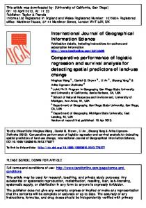
The numerical simulation is designed to compare the comparative classification accuracy of the conventional FLDA and the proposed robust FLDA. The group means and covariance matrices are fixed. The sample size are equal, n1 = n2 = 100 . The simulation is designed using scaled normal data and unscaled normal data. The sample data set used in this experiment is generated and is divided into training sample and validation sample; say 70% for training sample and 30% for validation. The focus of this study is to obtain the classification accuracy using hit ratio to access their comparative performance. The study criterion is to avoid upward biased when the training sample is used to build and validate the model. Based on this, the sample observations were reshuffled via zero one uniform distribution for each group. The reshuffled data set, say 70% was used for training and 30% was applied to validate the learned model. The experiment was replicated 100 times and the average number of runs reported (that is, mean of correct classification was reported). Table 1 below gives the classification rate of both techniques for unscaled normal data. This analysis supports the view that classical FLDA performs optimally when the assumptions of normality and equal variance covariance matrix hold, however the proposed approach based on these assumptions outperform the classical approach. Figure 1 and Figure 2 illustrate the separations between the group means. We observed that both techniques are well separated, this also support the classification rate. Table 1 Unscaled normal data
Observation (%) Method Correctly Classified Observation Misclassified CFLDA
99.7
0.3
RFLDA
100
0
216
11. 59
m ean t hr ee
9. 59 G r oup t wo
7. 59
m ean t wo 5. 59
3. 60
m ean one 1. 60 . 05
. 07
. 08
. 10
. 12
. 14
G r oup one
Figure 1 Unscaled normal data for CFLDA
. 14
m ean t hr ee
. 12
G r oup t wo . 10
m ean t wo
. 08
. 06
m ean one
. 04 1. 59
3. 59
5. 59
7. 59
9. 59
G r oup one
Figure 2 Unscaled normal data for RFLDA
217
11. 59
12. 80
m ean t hr ee
10. 65 G r oup t wo
8. 50
m ean t wo
6. 34
4. 19
m ean one 2. 04 . 49
. 66
. 83
1. 01
1. 18
1. 35
G r oup one
Figure 3 Scaled normal data for CFLDA
1. 37
m ean t hr ee
1. 19
G r oup t wo 1. 00
m ean t wo
. 81
. 63
m ean one
. 44 1. 99
4. 16
6. 32
8. 49
10. 66
12. 82
G r oup one
Figure 4 Scaled normal data for RFLDA
Table 2 below illustrates the classification rate of the classical FLDA and the robust FLDA for scaled normal data set. This experiment shows that classical FLDA perform poorly with scaled normal data, it also attest that the robust approach is actually robust in all conditions. We therefore conclude that in both situations the proposed approach outperformed classical approach. The classification error for the classical FLDA is 39.2 compared to 18.9 for the robust approach for scaled normal data. The conclusion is that 0.3 classification error for classical FLDA for the unscaled data is quiet reasonable and insignificant. The separability of the group means can be observed in Figures 3 and 4 respectively.
218
Table 2 Scaled normal data
Observation (%)
5
Methods Correctly Classified
Observations Misclassified
CFLDA
60.8
39.2
RFLDA
81.1
18.9
Conclusions
The proposed robust approach combines features of the conventional approach and weighting condition to robustify conventional sample mean and covariance matrix. The robust approach show high degree of classification and prediction accuracy. Simulation result shows that the new approach and the conventional approach perform similar for unscaled data. However, the robust approach outperforms the classical approach when simulation is performed with scaled normal data. The experiment also reveals the maximum separations between the group means. The results also affirm that classical FLDA perform optimally if normality and equal variance covariance matrix assumptions hold and poorly when the assumptions are violated. The classification rate investigated based on hit ratio shows that the robust approach performs better in both situations.
References [1] Fisher, A.R. The use of multiple measurements in taxonomic problems. Annals of Eugenics. 1936. 7:179-188. [2] Rao, C.R. The ultilization of multiple measurements in problems of biological classification. Journal of the Royal Statistical Society. 1948. 10:159-193. [3] Alvin, C.R. Methods of Multivariate Analysis. A John Wiley & Sons, Inc. 2002. [4] Hastie, T., Buja, A. and Tibshirani, R. Penalized discriminant analysis. The Annals of Statistics. 1995. 23:73-102. [5] Rousseeuw, P.J.Multivariate estimators with high breakdown point. Mathematical Statistics and its Applications. 1985. B: 283-297. [6] Kim, S.J., Magnani, A. and Boyd, S.P. Robust Fisher discriminant analysis. Advances in Neural Information Processing System. 2005. 18: 659-666. [7] Croux, C., Filzmoser, P. and Joossens, K. Classification efficiency for robust linear discriminant analysis. Statistical Sinica. 2008. 18: 581-599. [8] Pires, A.M. and Branco, J.A.Generalization of Fisher's linear discriminant. www.math.ist.utl.pt/~apires/PDF/APJB-RP96.pdf.1996. [9] Ella, R., Van Aelst, S. and Williem, G. The minimum weighted covariance determinant estimator. Metrika. 2009. 70: 177-204. [10] Hubert, M. and Van Driessen, K.Fast and robust discriminant analysis. Computational Statistics Data Analysis. 2004. 45: 301-320. [11] Basak, I. Robust M-estimation in discriminant analysis. The Indian Journal of Statistics. 1998. 60: 246-268. [12] Van Aelst, S. High breakdown robust multivariate methods. Statistical Science. 2008. 23: 92119. [13] Jin, J. and An, J.Robust discriminant analysis and its application to identify protein coding regions of rice genes. Mathematical Biosciences. 2011. 232: 96-100. 219
[14] Campbell, N.A. Robust procedures in multivariate analysis I : Robust covariance estimation. Applied Statistics. 1980. 29: 231-237. [15] Maronna, R.A. Robust M-estimators of multivariate location and scatter. The Annal of Statistics. 1976. 4: 51-67. [16] Davies, P.L. Asymptotic behaviour of S estimators of multivariate location paramters and dispersion matrices. The Annals of Statistics. 1987. 15:1269-1292. [17] Lopuhaa, H.P. On the relation between S estimators and M estimators of multivariate location and covariance. The Annals of Statistics. 1989. 17:1662-1683. [18] Rousseeuw, P.J. and Van Driessen, K. A fast algorithm for the minimum covariance determinant estimator. Technometrics. 1999. 41: 212-223. [19] Rousseeuw, P.J. and Van Zomeren, B.C. Unmasking multivariate outliers and leverage points. Journal of the American Statistical Association. 1990. 85: 633-651. [20] Johnson, A.R. and Wichern, D.W. Applied Multivariate Statistical Analysis. Prentice - Hall International, Inc. 1998. [21] Tatsuoka, M.M. and Lohnes, P.R. Multivariate Analysis Second Techniques for Educational and Psychological Research.New York: Macmillan Publishing Company. 1988. [22] William, R.D. and Matthew, G. Multivariate Analysis Methods and Applications. John Wiley & Sons. 1984. [23] Friedman, J.H. Regularized discriminant analysis. Journal American Statistical Association. 1989. 84:165-175. [24] Wu, G., Chen, C. and Yan, X. Modified minimum covariance determinant estimator and its application to outlier detection of chemical process data. Journal of Applied Statistics. 2011. 38(5):1007-1020. [25] Wei, W., Mo, Y., John, A.O. and Gustavo, K.R. Penalized Fisher discriminant analysis and its application to image-based morphometry. Pattern Recognition Letter. 2011. 32: 2128-2135. [26] Fauconnier, C. and Haesbroeck, G. Outlier detection with the minimum covariance determinant estimator in practice. Statistical Methodology. 2009.6:363-379. [27] Filzmoser, P. A multivariate outlier detection method. Computer wranglers.com/com531/handouts/Mahalanobis.pdf, 2005.1-5. [28] Kent, J.T. and Tyler, D.E. Redesceding M-estimates of multivariate location and scatter. The Annal of Statistics. 1991.19:2102-2119.
220