Abstract. A fuzzy partition assigns to each among n objects a distribution over a categories. Elementary linear algebraic methods permit to introduce and ...
On the comparison and representation of fuzzy partitions Fran¸cois Bavaud, University of Lausanne
Abstract A fuzzy partition assigns to each among n objects a distribution over a categories. Elementary linear algebraic methods permit to introduce and investigate concepts and properties such as a) variance and inertia decomposition; b) coarse- and fine-graining (nestedness); c) iteration of fuzzy partitions; d) stability of a group in regard to another partition; e) (euclidean embeddable) dissimilarities between objects; f) (euclidean embeddable) dissimilarities between partitions. Unweighted (R) or weighted (T , P ) object similarities are further investigated, and found to be related to the chi-square as well as to the indices of Gini, variety and Mirkin-Cherny-Rand. Weighted versions T and P differ for fuzzy partitions, allowing various non-equivalent constructions characterizing differing aspects of fuzzy partitions and possessing no formal analog at the crisp level1 .
1
Introduction and notations
Partitioning (deterministically) n objects consists in assigning each object i to a group j, among a possible groups; see e.g. Saporta pp. 210-224 (1990) or Mirkin pp. 229-246 (1996) for a classical, formal approach. A fuzzy partition consists of a probabilistic assignment of object i to groupPj, specified withPzij = “probability that object i belongs to group j”, obeying zij ≥ 0, aj=1 zij = 1 and ni=1 zij > 0 (absence of empty groups); see e.g. Bezdek (1981) for a presentation of the fuzzy context. Elementary algebra allows characterizing the combination, iteration or nesting of fuzzy partitions; associated operators, whose projective or Markov-like properties are exploited, possess simple interpretations in terms of dissimilarities between objects, yielding in turn euclidean embeddable dissimilarities between objects and even between partitions themselves. The present general framework suggests a certain view of the multivariate analysis of fuzzy partitions (=fuzzy categorical variables), that is of multiple fuzzy correspondence analysis.
2
Membership matrices
Definition 1 A (fuzzy) partition A of a set of n objects in a groups is defined by a (n × a) 1
The work has benefited from stimulating discussions with M.Rajman in the framework of the joint UNIL-EPFL “Clavis” project (2001).
1
A ≥ 0, (fuzzy) membership or indicator matrix such that zij P n A and nA j := i=1 zij > 0 for all j = 1, . . . , a.
Pa
A j=1 zij
= 1 for all i = 1, . . . , n
Definition 2 a) A deterministic or crisp partition obtains when zij = 1 or zij = 0 for 2 = z . In the case of a crisp partition, j(i) will denote the all i, j, or equivalently zij ij group to which i belongs. b) A partition is said to be full if Rank(Z) = a, and defective if Rank(Z) < a. Crisp partitions are full (since nj > 0). The uniform partition in a groups U(a) is defined U(a) by the (n × a) matrix zij = a1 for all i and j = 1, . . . , a. Uniform partitions are defective for a ≥ 2; the full case a = 1 defines the one-group partition O = U(1), with associated O = 1. The n-groups partition N is defined by the (n × n) (n × 1) membership matrix zi1 N = δ (or a permutation of it). identity matrix zij ij
2.1
Variance decomposition
Let X be a numerical variable with scores xi , i = 1, . . . , n. DefinePthe (fuzzy) average P P for z ¯j = n1 ni=1 xi , the j-th group as x ¯j := ni=1 nijj xi , and the total average as x ¯ = aj=1 fj x n where fj := nj . Define the total, within- and between-groups variances as n
1X var(x) := (xi −¯ x)2 n i=1
a
n
1 XX varW (x) := zij (xi −¯ xj )2 n j=1 i=1
varB (x) :=
a X
fj (¯ xj −¯ x)2
j=1
(1) Then the (fuzzy) variance decomposition formula var(x) = varW (x) + varB (x) holds. In particular, for fixed values {xi }, varW (x) is maximum for A = U(a) (for any a), and minimum for A = O.
2.2
Connected components
Define the (a × a) matrices B = (bjj 0 ) and N = (njj 0 ) as X B := Z 0 Z i.e. bjj 0 := zij zij 0 N := diag(10 Z) i.e. njj 0 := δjj 0 nj
(2)
i
where 1 is the (n × 1) unit vector. Note that Z 1 = 1 and Z 0 1 = N 1 , where 1 is the (m × 1) unit vector. Also, B −1 exists iff A is full. bjj 0 ≥ 0 constitutes an index of overlapping between groups j and j 0 and measures their common sharing of objects. Distinct groups j and j 0 with bjj 0 > 0 are said to be adjacent. Distinct groups j and j 0 related by a path bjk1 bk1 k2 . . . bkl j 0 > 0 of adjacent groups are connected. A set of connected groups constitutes an (irreducible) component, indexed by J = 1, . . . , c(A), where c(A) ≤ m is the number of irreducible components of the partition A, or, equivalently, the number of irreducible blocks of Z. One has: 2
c(A) = m Rank(Z) = m
2.3
⇔ ⇔
A is crisp A is full
⇔ ⇔
B=N exists
B −1
Iterated partitions
In view of the previous section, the matrix G := N −1 B is the identity iff is A crisp. In general, G generates iterated partitions: Definition 3 The r-th iterated membership Z (r) defining partition A(r) obtains as Z
(r)
:= Z G
r−1
G := N
−1
B = (gjj 0 )
gjj 0
n 1 X = zij zij 0 nj
(3)
i=1
Indeed, identity G 1 = 1 ensures the normalization Z (r) 1 = 1 : that is, Z (r) is the membership matrix associated to some (fuzzy) partition denoted A(r) . G 1 = 1 with gjj 0 ≥ 0 also shows G to be the (a × a) transition matrix of a Markov chain among groups j = 1, . . . , a: gjj 0 is the probability that, starting from group j in which one selects an individual i, one precisely gets group j 0 when further selecting a group from P (r) (r) individual i. Identity 10 ZN −1 Z 0 Z = 10 Z ensures nj := i zij = nj : the group sizes are thus unchanged by iteration. G is doubly stochastic, and made up of J = 1, . . . , c(A) irreducible doubly stochastic P (J) matrices G(J) , each with stationary distribution fj = nj /nJ where nJ := j∈J nj . Iterating partitions mixes the objects i among the various classes j of the same connected P (2) component J; for instance, zij = i0 j 0 zij 0 zi0 j 0 zi0 j /nj 0 . In the limit r → ∞, objects inside the same component J possess the same group membership: (∞)
gjj 0 =
nj 0 I(j 0 ∈ J(j)) nJ(j)
implying
(∞)
zij
=
nj I(i ∈ J(j)) nJ(j)
(4)
where I(E) denotes the characteristic function for event E, and J(j) denotes the component to which group j belongs. Partition A(∞) thus obtains by 1. first assigning individuals i to their component J(i); we denote this partition as A(0) , (0) with (n × c(A)) associated membership matrix ziJ = I(i ∈ J) 2. then choosing group j ∈ J(i) with probability nj /nJ(i) = fj /fJ(i) ; the (c(A) × a) n cg membership matrix associated to this component-group partition is zJj = nJj I(j ∈ J). By construction Z (∞) = Z (0) Z cg
Z (0) = Z Z gc
where
gc
ziJ := I(j ∈ J)
(5)
Partition A(∞) is defective iff A is fuzzy (since Rank(Z (∞) ) = c(A) < a), and full iff A is (r) (r) crisp. Crisp partitions are characterized by gjj 0 = gjj 0 = δjj 0 and zij = zij = I(i ∈ j). 3
Example 1 Consider the fuzzy partition A of n = 5 objects in a = 4 classes with 1 0 0 0 1.04 0.16 0 0 1.2 0 0 0 0.2 0.8 0 0 0.16 1.64 0 0 0 1.8 0 0 1 0 0 ZA = B= N = 0 0 0 0 0.4 0.4 0 0.8 0 0 0 0.6 0.4 0 0 0.4 0.8 0 0 0 1.2 0 0 0.2 0.8
13 15 4 45
G= 0 0
3
2 15 41 45
0 0
0 0 1 2 1 3
0 0 1
G
(∞)
2 2 3
0.4 0.6 0 0 0.4 0.6 0 0 = 0 0 0.4 0.6 0 0 0.4 0.6
Z
(∞)
=
0.4 0.6 0 0 0.4 0.6 0 0 0.4 0.6 0 0 0 0 0.4 0.6 0 0 0.4 0.6
Object comparisons
3.1
Object similarities
Let S = (sii0 ) denote a general (n × n) similarity matrix between objects, obeying sii0 ≥ 0, √ sii0 = si0 i and sii0 ≤ sii si0 i0 . Three natural candidates for S are provided by the (n × n) matrices R := ZZ 0 , T := ZN −1 Z 0 and (assuming the partition to be full, that is B −1 exists) P := ZB −1 Z 0 , namely2 rii0 :=
a X j=1
zij zi0 j
tii0 :=
a X zij zi0 j nj j=1
pii0 :=
a X
(−1)
zij bjj 0 zi0 j 0
(6)
j,j 0 =1
• R = (rii0 ) (the relation similarity matrix) yields, for a crisp classification, the indicator matrix of the relation “objects i and i0 belong to the same group”. P • T = (tii0 ) (the transition similarity matrix) satisfies i0 tii0 = 1: it is thus the transition matrix among objects of a doubly stochastic Markov chain; tii0 is the probability to jump from object i to object i0 when first selecting class j with probability zij and then selecting object i0 inside class j with probability zi0 j /nj . • P = (pii0 )(the projection similarity matrix) is a projection matrix (see theorem (1)). Also, P = T iff A is crisp; in other words, similarity matrices can be made simultaneously markovian and projective for crisp partitions only. Note that pii0 ≥ 0 can be √ violated (since B −1 possesses negative components); however, |pii0 | ≤ pii pi0 i0 holds. Theorem 1 a) T is a Markov transition matrix, with stationary uniform distribution πi = 1/n; its iterate obeys T 2 = T iff A is crisp (that iff T = P as well). 2 Equations (2) and (6) are somewhat reminiscent of the “Burt-Condorcet” duality in multiple correspondence analysis (see e.g. Marcotorchino (2000)). Recall however the latter to refer to p ≥ 2 crisp partitions, rather than one fuzzy partition as in the present case.
4
b) In general, however, 1 ≤ Tr(T 2 ) ≤ Tr(T ) ≤ a, with Tr(T ) = 1 iff A is the uniform partition U(a) (for any a), and Tr(T ) = a iff A is crisp, in which case T = P . c) P exists iff A is full, in which case P 2 = P and Tr(P ) = a. Proof of theorem 1
a) obtains from c) below; recall T = P in the crisp case. 2 zij ij nj .
2 ≤ z Tr(T ) = a holds as a consequence of zij ij P 1 2 with equality iff A is crisp. Tr(T ) = 1 obtains from Jensen’s inequality n i zij ≥ P { n1 i zij }2 with equality iff A is the uniform partition.
b) by definition, Tr(T ) =
P
Inequality (zij − zi0 j )2 zij 0 zi0 j 0 ≥ 0 holds in general, while (zij − zi0 j )2 zij 0 zi0 j 0 = 0 for all i, i0 , j, j 0 iff A is crisp. Summing the latter yields 2 z 0z 0 0 2 X zij X zij X zij zi0 j zij 0 zi0 j 0 ij i j ≤ = = Tr(T ) Tr(T ) = nj nj 0 nj nj 0 nj 0 0 0 0 2
ij
ii jj
ii jj
which demonstrates that T 2 6= T if A is not crisp. On the other hand, T = P if A is crisp, and thus T 2 = T . c) P 2 = ZB −1 Z 0 ZB −1 Z 0 = ZB −1 BB −1 Z 0 = ZB −1 Z 0 = P ; also, Tr(P ) = Tr(ZB −1 Z 0 ) = Tr(B −1 Z 0 Z) = Tr(B −1 B) = Tr I = a.
3.2
Iterated object similarities
Higher order similarities can be constructed as R(r) := Z (r) (Z (r) )0 , T (r) := Z (r) (N (r) )−1 (Z (r) )0 and (for a full partition) P (r) := Z (r) (B (r) )−1 (Z (r) )0 , where Z (r) := Z Gr−1 , B (r) := (Z (r) )0 Z (r) and N (r) := diag(10 Z (r) ). Theorem 2 For r ≥ 0, T (r) = T 2r−1 and (for a full partition) P (r) = P . Proof of theorem 2 P (r+1) = Z (r+1) (B (r+1) )−1 (Z (r+1) )0 = Z (r) N −1 B[BN −1 B (r) N −1 B]−1 BN −1 (Z (r) )0 = = Z (r) N −1 BB −1 N (B (r) )−1 N B −1 BN −1 (Z (r) )0 = Z (r) (B (r) )−1 (Z (r) )0 = P (r) Using N (r) = N , identity T (r) = T 2r−1 is proved similarly.
3.3
Object distances
Matrices R, T and P are three instances of positive-definite similarity matrices S = (sii0 ) between objects i and i0 , from which a squared euclidean distance can be constructed as S := (dS )2 = s + s 0 0 − 2s 0 (Schoenberg 1935; Gower 1982). Explicitly Dii 0 ii ii ii jj 0 R Dii 0 =
X j
(zij − zi0 j )2
T Dii 0 =
X (zij − zi0 j )2 nj j
P Dii 0 =
X
(−1)
(zij − zi0 j )bjj 0 (zij 0 − zi0 j 0 )
jj 0
(7) 5
Theorem 3 : for a crisp partition: 1 nj
R = DT = DP = 0 Dii 0 ii0 ii0
rii0 = tii0 = pii0 = 0
R = 2 DT = DP = Dii 0 ii0 ii0
rii0 = 1 tii0 = pii0 =
for i, i0 ∈ j 1 nj
+
1 nj 0
for i ∈ j, i0 ∈ j 0 with j 6= j 0
N = tN = pN = δ 0 ; r O = 1 and tO = pO = 1 . In particular, rii 0 ii ii0 ii0 ii0 ii0 ii0 n
Proof of theorem 3 : straightforward. P Let aj ≥ 0 with j aj = 1 be the membership profile of some object a; for instance, P n gj = n1 i zij = nj represents the membership profile of the gravity center g. Then squared S can be defined by the substitution z 0 → a in (7). Define distances Dia j ij I2S =:
1 X S D 0 2n2 0 ii
(pair inertia)
I1S (a) =:
1X S Dia n
(central inertia with center a)
i
i,i
(8) Then, for S = R, T or P , S I1S (a) = I1S (g)+Dag
I2S = I1S (g) (weak Huygens principle) (9) (see e.g. Bavaud (2002)). The pair inertia I2S = P I1S (g) constitutes an index of classificatory diversity; for crisp partitions A, one gets I2R = aj=1 fj (1 − fj ) (Gini diversity index) and I2T = I2P = (a − 1)/n. (strong Huygens principle)
As it it well known (classical MDS), coordinates xSiα realizing an euclidean representation P S S of the objects i = 1, . . . , n in dimensions p α = 1, . . . , a − 1 (that is satisfying Dii0 = α (xiα − xSi0 α )2 ) can be obtained as xSiα := λSα uSiα , where the λSα are the eigenvalues and the uSiα the eigenvectors occurring in the spectral decomposition S = U S ΛS (U S )0 . Example 1 .2 .2 .68 R= 0 .8 0 0 0 0
1, continued: the (5 × 5) corresponding similarity matrices are .98 .12 −.10 0 0 .83 .17 0 0 0 0 0 0 .17 .39 .44 .12 .40 0 0 .48 0 0 .8 0 0 .62 0 0 1 0 0 0 0 P = −.10 .48 T = 0 .44 .56 0 0 .52 .44 0 0 .58 .42 0 0 0 1 0 0 0 0 .42 .58 0 0 0 0 1 0 .44 .68
with associated squared distances between objects 0 1.28 0 .89 2 1.52 1.68 DR =
1.28 2 1.52 1.68
0 .08 1.2 1.36
.08 0 1.52 1.68
1.2 1.52 0 .32
1.36 1.68 .32 0
T D =
.89 1.39 1.42 1.42
6
0 .06 .97 .97
1.39 .06 0 1.14 1.14
1.42 .97 1.14 0 .33
1.42 .97 1.14 .33 0
P D =
0 1.14 1.79 1.98 1.98
1.14 0 .07 1.40 1.40
1.79 .07 0 1.62 1.62
1.98 1.40 1.62 0 2
1.98 1.40 1.62 2 0
Spectral decomposition of S yields the corresponding (5 × 4) coordinates X S = (xSiα ): .58 −.71 0 0 −.12 .98 .24 .97 0 0 .82 .58 .61 0 0 0 .24 0 0 .19 R T P 0 0 X = .58 .47 0 0 X = .79 −.24 X = .97 −.24 0 0 0 .66 −.30 0 −.71 .29 0 0 0 0 .79 .25 0 0 −.71 −.29 0 0
4
Nested partitions: coarser and finer
Definition 4 Partition B (defined by the (n × b) membership matrix Z B ) is coarser than partition A (defined by the (n × a) membership matrix Z A ), or, equivalently, A is finer AB ) is a (a × b) class membership than B, noted B ≤ A, if Z B = Z A W AB where W AB = (wjk P b AB AB ≥ 0 and matrix such that wjk k=1 wjk = 1. Theorem 4
a) The relation “B ≤ A” is a partial order
b) its minimal element is the one-group partition O c) its maximal element is the n-groups partition N d) if B ≤ A (with A and B both full) then P A P B = P B P A = P B . AA = δ ). Also, B ≤ A and Proof of theorem 4 a) By definition, A ≤ A (with wjk jk C ≤ B entail C ≤ A (with W AC = W AB W BC ).
b) for any A, Z O = Z A W AO with wjAO = 1 for all j = 1, . . . , a. N B = zB . c) for any B, Z B = Z N W N B with wij ij
d) Z A W AB = Z B and B A = (Z A )0 Z A yield P A P B = Z A (B A )−1 (Z A )0 Z B (B B )−1 (Z B )0 = = Z A (B A )−1 (Z A )0 Z A W AB (B B )−1 (Z B )0 = Z B (B B )−1 (Z B )0 = P B | {z } I
Identity P B P A = P B is demonstrated analogously. Theorem 5 For r ≥ 1, the sequence of partitions A(r) associated with the iterated memberships Z (r) (definition 3) is decreasing (that is A(r+1) ≤ A(r) ). Its limit A(∞) is given by the membership matrix Z (∞) defined in (4). Also, A(∞) ≤ A(0) ≤ A. (r+1) = Z (r) G (equation (3)), Proof of theorem 5 The first two assertions follow Pafrom Z where G is a (a × a) non-negative matrix obeying j 0 =1 gjj 0 = 1 together with properties listed in section (2.3). The last assertion is a direct consequence of (5).
7
0 0 0 1 0
0 0 0 0 1
5
Comparison and representation of partitions
5.1
The general case: euclidean visualization
B B Definition 5 Let S A = (sA ii0 ), respectively S = (sii0 ), be the (n × n) similarity matrix associated to partition A, respectively partition B. The corresponding (squared) distance S DA,B between two partitions A and B is defined as S DA,B :=
X
B 2 A B 2 A 2 B 2 A B (sA ii0 − sii0 ) = Tr(S − S ) = Tr((S ) ) + Tr((S ) ) − 2Tr(S S )
(10)
ii0 S The distance DA,B possesses all the properties of a squared euclidean distance, in particular the embeddability property. Then classical MDS applied on matrix DS yields a low-dimensional euclidean visualization of the distances between partitions, each partition being represented by a point (see figure 1).
Example 2 Consider n = 5 objects. Define • A as the fuzzy partition of example 1 • B as the partition A(0) in connected components (namely (123; 45)) • C as the crisp partition (12; 345) • D ≡ N as the n-groups partition (1; 2; 3; 4; 5) • E ≡ O as the one-group partition (12345) • F ≡ A(∞) as the limiting iterated partition:
Z
A
=
Z
D
=
1 0 0 0 0
1 0 0 0 0.2 0.8 0 0 0 1 0 0 0 0 0.6 0.4 0 0 0.2 0.8 0 1 0 0 0
0 0 1 0 0
0 0 0 1 0
0 0 0 0 1
Z = B
Z = E
1 1 1 1 1
8
1 1 1 0 0
0 0 0 1 1
Z = C
Z
F
=
1 1 0 0 0
0 0 1 1 1
0.4 0.6 0 0 0.4 0.6 0 0 0.4 0.6 0 0 0 0 0.4 0.6 0 0 0.4 0.6
The corresponding dissimilarities (10) DS between partitions (listed in alphabetical order) are3 0 4.42 7.62 2.18 16.42 1.43 4.42 0 8 8 12 3.00 7.62 8 0 8 12 7.16 R D = 2.18 8 8 0 20 3.32 16.42 12 12 20 0 15.00 1.43 3.00 7.16 3.32 15.00 0 T D =
5.2
0 0.63 1.37 1.74 1.74 0.63 0.63 0 1.11 3 3 0 1.37 1.11 0 3 3 1.11 1.74 3 3 0 0 3 1.74 3 3 0 0 3 0.63 0 1.11 3 3 0
D = P
0 2 2.63 1 1 2 0 1.11 3 3 2.63 1.11 0 3 3 1 3 3 0 0 1 3 3 0 0
The full case for S = P
P = When A and B are both full, P A and P B are well defined and theorem (1) yields DA,B A B A B Tr(P + P − 2 P P ). If B ≤ A in addition, the distance further expresses (theorem P = Tr(P A ) − Tr(P B ) = a − b: the distance between two nested, full partitions (4)) as DA,B is measured by the difference of their number of groups. In particular P = DP P • DA,C A,B + DB,C if C ≤ B ≤ A or A ≤ B ≤ C P P = a − 1 and DN • for A full, DO,A ,A = n − a P • for A full, DA (0) ,A = a − c(A)
5.3
The crisp case: chi-square and Mirkin-Cherny-Rand indices
Let A and and P b non-empty classes. Let P BAbe two crisp partitions possessing respectively a B := B nA := z be the number of objects in class j of A, n j i ij i zik be the number of k P A B objects in class k of B, and define nA,B i zij zik as the number of objects both in class jk := j of A and k of B. P P P A B P A,B 2 A zA zB zB = Definition 6 : NA,B := ii0 jj 0 zij ii0 rii0 rii0 = jk (njk ) denotes the i0 j ij 0 i0 j 0 number of pairs (distinct or not) which are simultaneously classified in the same group j of A and k of B. 3
as F is defective, P F is not defined.
9
1.4
c
2.0 1.5
factor 2 (31%)
factor 2 (16%)
2.5
d
1.0 .5
b
0.0 -.5 -1.0 -5
e -4
-3
-2
fa
-1
0
1.0
b f
.8 .6 .4 .2
d e
-.2 -1.5
1
a
0.0
factor 1 (66%)
-1.0
-.5
0.0
.5
factor 1 (60%)
d e
1.2
factor 2 (30%)
c
1.2
1.0 .8 .6 .4
c
.2 0.0 -.2 -.4 -2.0
a b
-1.5
-1.0
-.5
0.0
.5
factor 1 (63%) S , Figure 1: Euclidean visualization (classical MDS) of the distances between partitions DA,B Page 1 for S = R (top left), S = T (top right) and S = P (down). Coordinates for D and E are identical in the T − and P −representation; also, coordinates for B and F are identical in the T −representation. Recall that F is defective and hence not P −representable.
10
P A 2 P B 2 A,B 2 njk ≤ nA,A = (nA j ) , and thus NA,B ≤ NA,A = j (nj ) (and NA,B ≤ NB,B = k (nk ) ), jj with equality iff the two (crisp) partitions A and B are identical. Theorem 6 R DA,B = NA,A + NB,B − 2NA,B
where χ2A,B :=
Pa
j=1
Pb
T P DA,B = DA,B = (a − 1) + (b − 1) −
nj• n•k 2 ) n nj• n•k n
(njk −
k=1
table njk = nA,B jk .
2 2 χ n A,B
(11)
is the chi-square associated to the contingency
R The quantity n12 DA,B is called “relative symmetric-difference distance” by Mirkin and Cherny (1970). Its complement to unity4 is known as the “Rand similarity index” (Rand 1971).
Proof of theorem 6 : the first identity follows from X XX X R A B 2 A A B B 2 DA,B = (rii ( zij zi0 j − zik zi0 k ) = 0 − rii0 ) = ii0
ii0
j
k
X XX X A A B B A A A A B B B B zi0 k zik0 zi0 k0 − 2 zij zi0 j zik zi0 k ] = = [ zij zi0 j zij 0 zi0 j 0 + zik ii0
=
X
δjj 0 nA j δjj 0
nA j
+
jj 0
X
jj 0
δkk0 nB k δkk0
j 0 k0
nB k
−2
X
kk0
2 (nAB jk )
jk
=
X
2 (nA j )
+
j
jk
X
2 (nB k) − 2
X
2
(nAB jk )
jk
k
P = Tr(P A ) + Tr(P B ) − 2Tr(P A P B ) = a + b − 2 Tr(P A S B ) and and the second from DA,B 2 AzA A A X X zij X (nA,B 1 i0 j zi0 k zik jk ) Tr(P P ) = = = 1 + χ2A,B A B A B n nj nk nj nk jk ii0 jk A
5.4
B
The crisp case: instability of a group relatively to another partition
Let A and B be two crisp partitions whose non-empty groups are respectively indexed by j = 1, . . . , a and k = 1, . . . , b; let nj := nA j > 0 denote the number of objects i ∈ j. Theorem 7 R DA,B =
a X
ρB j
2 B B ρB j := nj − 2αj + βj
=
P DA,B
=
a X
τjB
τjB := 1 − 2γjB + δjB
B rii 0
βjB :=
γjB :=
1 X B pii0 nj 0
at least in the variant restricted to the contribution of distinct pairs only.
11
X
B rii 0
(12)
i∈j;i0
i,i ∈j
j=1 4
X i,i0 ∈j
j=1
T DA,B
αjB :=
δjB :=
X i∈j
pB ii (13)
B ρB j and τj constitute measures of the instability of group j (of partition A) relatively to partition B; by construction, their sum over the groups j = 1, . . . , a yields the (squared) distance between partitions A and B. Note that:
• n2j is the number of (distinct or not) pairs of objects in j • αjB is the number of pairs in j which are also classified in the same group k of B • βjB is the number of pairs classified in the same group k of B, such that the first object of the pair belongs to j. 2 B As n2j ≥ αjB and βjB ≥ αjB , one has ρB j ≥ 0 with equality iff nj = αj (all pairs in j are pairs for B) and βjB = αjB (all pairs (i, i0 ) for B such that i ∈ j satisfy i0 ∈ j). Also:
• γjB is a measure of the pair cohesion in B “as seen from j” • δjB is a measure of the fineness of groups of B “as seen from j”. P A B B B B B Properties pB i0 pii0 = 1 entail γj ≤ δj and γj ≤ 1, and thus τj ≥ 0. ii0 ≤ pii and Proof of theorem 7 X XXX X X X R A B 2 A A B B B B DA,B = (rii [rii [n2j − 2 rii rii 0 − rii0 ) = 0 − 2rii0 rii0 + rii0 ] = 0 + 0] ii0
T DA,B =
X
j
i0
i,i0 ∈j
j
i∈j;i0
X XX X X X 2 X B B A B + p pB [ + pA − 2 p p ] = p [1 − 0 0 0 ii ] ii ii ii ii ii nj 0
B 2 (pA ii0 − pii0 ) =
ii0
j
A )2 = r A and where (rii 0 ii0
i∈j
i∈j
A 2 i0 (pii0 )
P
i∈j
i∈j
j
i,i ∈j
i∈j
= pA ii = 1/nj(i) have been used.
Example 3 : the instability of class j with regard to the n-groups partition B = N is: • ρN j = nj (nj − 1)
(large groups are unstable)
• τjN = nj − 1
(large groups are unstable)
Its instability with regard to the one-group partition B = O is: • ρO j = (n − nj ) nj • τjO =
n−nj n
= 1 − fj
(medium groups are unstable) (small groups are unstable).
12
6
References • BAVAUD, F. (2002): “Quotient Dissimilarities, Euclidean Embeddability, and Huygens’ Weak Principle”. In K. Jajuga and al. (Eds.): Classification, Clustering, and Data Analysis. Springer, 195-202 • BEZDEK, J. (1981): “Pattern recognition with Fuzzy Objective Function Algorithms”, Plenum Press • GOWER, J.C. (1982): “Euclidean distance geometry”. The Mathematical Scientist, 7, 1-14 • MARCOTORCHINO, J.F. (2000): “Dualit´e Burt-Condorcet: relation entre analyse factorielle des correspondances et analyse relationnelle”. In J.Moreau and al. (Eds.): L’analyse des correspondances et les techniques connexes. Springer, 211-227 • MIRKIN, B. (1996): “Mathematical Classification and Clustering”, Kluwer • MIRKIN, B. and CHERNY, L.B. (1970): “On a distance measure between partitions of a finite set”, Automation and Remote Control, 31, 786-792 • RAND, W.M. (1971): “Objective criteria for the evaluation of clustering methods”, Journal of the American Statistical Association, 66, 846-850 • SAPORTA, G. (1990): “Probabilt´es, analyse de donn´ees et statistique”, Editions Technip, Paris • SCHOENBERG, I.J. (1935): “Remarks to Maurice Fr´echet’s article “Sur la d´efinition axiomatique d’une classe d’espaces vectoriels distanc´es applicables vectoriellement sur l’espace de Hilbert””. Annals of Mathematics, 36, 724-732
13