the claimed result. Fix an rsm M and an L(3) formula Ï. Our first goal is to define a finite certificate for a run that will be used in the argument to show membership ...
On the Complexity of Ltl Model-Checking of Recursive State Machines? Salvatore La Torre1 and Gennaro Parlato1,2 1
2
Universit` a degli Studi di Salerno, Italy University of Illinois at Urbana-Champaign, USA
Abstract. Recursive state machines (rsms) are models for programs with recursive procedural calls. While Ltl model-checking is Exptimecomplete on such models, on finite-state machines, it is Pspace-complete in general and becomes Np-complete for interesting fragments. In this paper, we systematically study the computational complexity of modelchecking rsms against several syntactic fragments of Ltl. Our main result shows that if in the specification we disallow next and until, and retain only the box and diamond operators, model-checking is in Np. Thus, differently from the full logic, for this fragment the abstract complexity of model-checking does not change moving from finite-state machines to rsms. Our results on the other studied fragments confirm this trend, in the sense that, moving from finite-state machines to rsms, the complexity of model-checking either rises from Pspace-complete to Exptimecomplete, or stays within Np.
1
Introduction
Linear temporal logic (Ltl) is a specification language commonly used for expressing correctness requirements of reactive systems [10, 11]. An Ltl formula is built from atomic propositions, boolean connectives, and temporal modalities such as next, diamond, box, and until, and is interpreted over infinite sequences of states which model computations of reactive programs. A typical temporal requirement is “every request p is followed by a response q,” and can be expressed in Ltl as 2 ( p → 3 q ). Given an abstract model M of a reactive system and an Ltl formula ϕ, Ltl model-checking asks whether an infinite computation of M satisfying ϕ exists. When M is finite-state, this decision problem is Pspace-complete [12]. Despite the high computational complexity, solutions to Ltl model-checking are implemented in verification tools and successfully applied in practice (see [5, 9]). The control flow of programs with recursive procedure calls can be naturally captured with recursive state machines (rsms). In an rsm, vertices can either be ordinary states or can correspond to invocations of other state machines in a potentially recursive manner. We recall that rsms correspond to pushdown ?
This research was partially supported by the MIUR grant ex-60% 2005, Universit` a degli Studi di Salerno.
systems, and the related model-checking problem has been extensively studied in the literature [1, 4, 8, 13]. Among the many interesting results, we recall that Ltl model-checking of rsms is Exptime-complete [4]. On finite-state systems, the computational complexity of model-checking for meaningful Ltl fragments improves (see [6]). In particular, for the logic of all formulae obtained by allowing an arbitrary nesting of diamond and box operators, which we denote with L(3), model-checking is Np-complete [12]. This fragment is very rich and can express many interesting properties of reactive systems, such as liveness (as the above response property) but also safety, fairness, and others. In this paper, we systematically study the computational complexity of modelchecking rsms with respect to specifications from natural syntactic fragments of Ltl. Our goal is the discovery of more efficient algorithms for interesting classes of specifications and a better understanding of the computational complexity of this decision problem. The main result of this paper concerns the computational complexity of model-checking rsms with respect to L(3) specifications. We show that this problem is in Np, that matches the known lower bound for finite-state machines. Thus, differently from full Ltl, the computational complexity of L(3) model-checking stays unchanged while moving from finite-state systems to rsms. Considering the simple structure of L(3) models [12], this result may not seem surprising. However, the effects of mixing this logic with the use of a stack were not completely clear. In the Exptime-hardness proof for Ltl [4], the stack of the model is used to linearize computations of an alternating Turing machine working in polynomial space and this basically allows the authors to carry over the Pspace-hardness proof of the Ltl model-checking of finite-state machines. Moreover, the expressiveness of L(3) combined with the alternation provided by a 2-player game graph suffices to prove a matching lower bound for deciding full Ltl games [3]. To show Np membership for the model-checking of rsms with respect to L(3) specifications, we define a certificate (a finite sequence of alternate nodes and set of nodes of the rsm) and then show that the problem can be reduced to answering two distinct queries: (1) checking that the certificate satisfies the given formula, and (2) checking that there exists a run of the given rsm which matches the certificate. To complete the Np membership argument we also show that we only need to investigate certificates of length bounded by the size of the formula. Observe that the smallest model of an L(3) formula among all the runs of an rsm can be of size over-polynomial, thus looking for an abstract representation of runs is needed and clearly the arguments used in showing Np membership of this problem on finite Kripke structures [12] cannot be applied here. The other results of this paper concern the model-checking of rsms with respect to specifications expressed in other syntactic fragments of Ltl. For fragments whose model-checking problem on finite-state machines is Pspacecomplete, we show Exptime-hardness, and therefore the model-checking problem is Exptime-complete. For fragments whose model-checking problem on finite-state machines is Np-complete, we instead give an Np upper bound. Remarkably, for some of these fragments we re-use results shown to prove Np
membership for L(3). All the results are summarized in a table in the concluding section.
2 2.1
Logic and Models Propositional Linear Temporal Logic
In this section, we briefly recall the logic Ltl and Ltl model-checking (see [7]). Given a set of atomic propositions AP , a propositional linear temporal logic (Ltl) formula is composed of atomic propositions from AP , the boolean connectives negation (¬), conjunction (∧) and disjunction (∨), the temporal operators next ( f), diamond (3), box (2), and until ( U). Formulae are built up in the usual way from these operators and connectives, according to the following grammar ϕ := p | ¬ϕ | ϕ ∧ ϕ | fϕ | ϕ U ϕ, where p is an atomic proposition of AP . The other formulae can be introduced as abbreviations in the usual way. In particular, the diamond operator is a restricted form of until (i.e., 3 ϕ ≡ true U ϕ holds), and the box operator expresses the logical negation of the diamond operator (i.e., 3 ϕ ≡ ¬(2 ¬ϕ) holds). Ltl formulae are interpreted on linear-time structures. A linear-time structure (or simply a structure) is a pair (π, lab π ) where π is an ω-sequence π = s0 s1 s2 . . . of states and lab π is a mapping lab π : {s0 , s1 , s2 , . . .} → 2AP labeling each state si with the set of propositions that hold at si . Let π be a structure, i ∈ N0 be a position, and ϕ an Ltl formula. The satisfaction relation |= is inductively defined as follows. – – – – –
def
(π, i) |= p ⇔ p ∈ lab π (si ); def (π, i) |= ¬ϕ ⇔ (π, i) |= ϕ holds false (i.e., (π, i) 6|= ϕ); def (π, i) |= ϕ ∧ ψ ⇔ (π, i) |= ϕ and (π, i) |= ψ; def (π, i) |= fϕ ⇔ (π, i + 1) |= ϕ; def (π, i) |= ϕ U ψ ⇔ ∃j ≥ i such that (π, j) |= ψ, and ∀k ∈ [i, j −1], (π, k) |= ϕ;
When (π, 0) |= ϕ, we also write π |= ϕ and say that π is a model of ϕ. An Ltl-formula ϕ is satisfiable if there exists a model of ϕ. Given an Ltl formula ϕ, we denote with |ϕ| its length. We denote with L(3) the Ltl fragment that allows only 3 and 2 as temporal operators (no next or until operators are allowed). Given a set of atomic propositions AP , a Kripke structure over AP is a tuple M = (S, ∆, lab, I) where: S is a (possibly infinite) set of states; ∆ ⊆ S × S is a transition relation; lab : S → 2AP is a labeling function that associates with each state s a set of atomic propositions lab(s) (meaning that the atomic propositions that hold true at s are exactly those in lab(s)); I ⊆ S is the set of the initial states of M . We say that M is a finite Kripke structure when S is finite. A run or path of M is a (finite or infinite) sequence of states π = s0 s1 . . . of M , such that s0 ∈ I
and (si , si+1 ) is a transition of M , with i ≥ 0. Notice that, each run in M is a linear-time structure. We write M |= ϕ when there exists an infinite run π of M such that π |= ϕ. The model-checking problem is: “given a Kripke structure M and an Ltl formula ϕ, does M |= ϕ?” With |M | we denote the size of M , that is |S| + |∆|. In the following, we use the result. Theorem 1 ([12]). The model-checking problem of a finite Kripke structure against an L(3) formula is Np-complete. 2.2
Recursive State Machines
In this section, we recall the recursive state machines (rsms) introduced in [1]. Syntax. Let IM = {1, . . . , k}. A recursive state machine (rsm) M over a set of atomic propositions AP is a tuple (M1 , . . . , Mk ), where Mh = (Nh , Bh , Yh , En h , Ex h , Eh , true h ), for h ∈ IM , is a module and consists of the following components: – – – –
A finite nonempty set of nodes Nh , and a finite set of boxes Bh . A labeling Yh : Bh → IM that assigns to every box a module index. A set of entry nodes En h ⊆ Nh , and a set of exit nodes Ex h ⊆ Nh . Let Calls h = {(b, e)|b ∈ Bh , e ∈ En j , j = Yh (b)} denote the set of calls of Mh , and Retns h = {(b, x)|b ∈ Bh , x ∈ Ex j , j = Yh (b)} denote the set of returns in Mh . Then, Eh ⊆ ((Nh ∪ Retns h ) × (Nh ∪ Calls h )) is the set of edges of Mh . – A labeling function true h : Nh → 2AP that associates a set of atomic propositions to each node of Mh .
We assume that NS 1 , . . . , Nk (respectively, B1 , . . . , Bk ) are pairwiseSdisjoint. We define with N = i∈IM Ni the set of all S nodes of M, with B = i∈IM Bi the set of all boxes of M, and with E = i∈IM Ei the set of all edges of M. Also, Y : B → IM denotes the extension of all the functions Yh , h ∈ IM , and true : N → 2AP denotes the extension of all the functions true h (h ∈ IM ). Module Mk is the initial module of M. Fig. 1 illustrates the definition. The rsm has two modules. The module M1 has 5 nodes, of which e1 and e2 are the entry nodes and x1 and x2 are the exit nodes, and two boxes, of which b1 is mapped to module M2 and b2 is mapped to M1 . The entry and exit nodes are the control interface of a module by which it can communicate with the other modules. Intuitively, think of modules as procedures, and an edge entering a box invoking the procedure associated with the box. Semantics. With each module of an rsm, we associate a Kripke structure by recursively substituting each box by the module referenced by the box. Formally, we associate to the module Mh the Kripke structure MhF = (Sh , ∆h , lab h , Ih ), called the expansion or the flat of Mh in M, as follows. The states Sh of MhF are elements of the form hαui where αu ∈ B ∗ × N and either
M2
M1 b 2 : M1
e1
x3
x1
v e2
u
e3 b 1 : M2
x2
b 3 : M1
x4
Fig. 1. A sample recursive state machine.
– α = � and u ∈ Nh , or, – α = b1 . . . b` (with ` ≥ 1), b1 ∈ Bh , bi+1 ∈ BY (bi ) for every i ∈ [1, ` − 1], and u ∈ NY (b` ) . The initial states of MhF are Ih = {hei|e ∈ En h }. The labeling function is lab h (hαui) = true(u). In the following, for the ease of presentation, we also denote the states of M of the form hαbui, where (b, u) is a call or a return, as hα(b, u)i. Therefore, states corresponding to calls or returns will have two representations and of the two we will always use the more convenient one, as for the following definition. Given two states X, X 0 of MhF , we define the transition relation ∆h as: (X, X 0 ) ∈ ∆h iff X = hαui, X 0 = hαvi, and (u, v) is an edge of M. (Note that in order to make the above definition consistent, we implicitly use the representation of the form hβ(b, z)i for X, if (b, z) is a return, and for X 0 , if (b, z) is a call, and the standard representation in all the other cases.) The expansion MkF of the initial module of M is also denoted MF . Given a state X = hαui with u ∈ N , we denote with node(X) the node u, and say that u is the node of X. An rsm M satisfies an Ltl formula ϕ, written M |= ϕ, iff MF |= ϕ. The model-checking problem of an rsm M against an Ltl formula ϕ is to determine whether M satisfies ϕ. The following result holds. Theorem 2 ([1]). The problem of model-checking an rsm against an Ltl formula is Exptime-complete.
3
The Complexity of L(3) Model-Checking on rsms
In this section we show that model-checking of L(3) formulae against rsms is Np-complete. We prove first some preliminary results and then use them to argue the claimed result. Fix an rsm M and an L(3) formula ϕ. Our first goal is to define a finite certificate for a run that will be used in the argument to show membership in Np. An M-sequence of length ` is a sequence γ = u0 , U1 , u2 , U3 , . . . , u2` , U2`+1 such that u0 , u2 , . . . , u2` are M nodes, and U1 , U3 , . . . , U2`+1 are sets of M nodes. For
a run π of MF and an M-sequence γ as above, we say that π and γ match if π can be factored as X0 π1 X2 π3 . . . X2` π2`+1 where X2i are states, π2i+1 are runs, node(X2i ) = u2i , and all the nodes of states occurring in π2i+1 belong to U2i+1 , for every i ∈ [0, `], and for all u ∈ U2`+1 , u is the node of infinitely many states in π2`+1 . It is crucial for our argument to be able to decide in polynomial time whether there exists an MF run that matches a given M-sequence γ. We can construct a simple B¨ uchi automaton A of size linear in the sizes of M and γ which accepts infinite sequences matching γ. Therefore, the above problem reduces to checking for emptiness the intersection of M and A. Thus, by the results shown in [1, 8] we have: Lemma 1. Given an M-sequence γ, deciding if there exists a run of MF matching γ can be done in deterministic polynomial time in the size of M and the length of γ. The second important step in our argument for showing Np membership consists of defining a notion of satisfiability of formulae on M-sequences that can be checked efficiently and that is sufficient to show satisfiability on a matching run of MF . Fix an M-sequence γ = u0 , U1 , u2 , U3 , . . . , u2` , U2`+1 . We denote with BD(ϕ) the set of all the box/diamond sub-formulae ψ of ϕ, and for a linear structure π = s0 s1 s2 . . ., we denote with BD ϕ π (si ) the set of all formulae ψ of BD(ϕ) such that (π, i) |= ψ. We say that γ satisfies ϕ if: 1. the sequence π = u0 u2 . . . u2` π 0 is a model of ϕ, where π 0 is any infinite sequence over U2`+1 such that each u ∈ U2`+1 occurs as the node of infinitely many states of π 0 ; 2. for every i ∈ [1, `] and for every u in U2i−1 , BD πϕˆ (u) = BD ϕ π (u2i ) where π ˆ = uu2i . . . u2` π 0 . The following proposition elaborates on some results shown in [12] for the logic we are considering. Proposition 1. Let π = s0 s1 s2 . . . be a structure and π 0 be the suffix of π such that for each state s in π 0 there are infinitely many states s0 in π 0 such that lab π (s) = lab π (s0 ).1 1. For an L(3) formula ϕ, the set of ϕ sub-formulae that hold at a state si depends only on the atomic propositions that hold at si and the box/diamond sub-formulae that hold at si+1 along π. ϕ 00 0 00 0 0 2. For ϕ ∈ L(3), BD ϕ π (s )BD π (s ) for every pair of states s , s within π . The following lemma states that satisfaction of a formula ϕ on a given Msequence can be efficiently verified. 1
Note that such a suffix of π always exists since 2AP is finite.
Lemma 2. Given an L(3) formula ϕ and an M-sequence γ, checking that γ satisfies ϕ can be done in polynomial time. Proof. Checking part 1 of the definition of satisfiability on M-sequences is trivial and can be done in linear time (see [12]). From Proposition 1, we can start ϕ 0 computing BD ϕ π (u) for a u in π , and then we compute the subsets BD π (u2i ) for i = `, . . . , 0. Therefore, the lemma is proved. t u A crucial step in our argument for showing membership in Np is to prove that we can answer to our model-checking question simply searching for an Msequence γ which satisfies the given formula and checking for the existence of a run of MF matching γ. The next two lemmas prepare such a result. Lemma 3. If an M-sequence γ satisfies ϕ then each run of MF which matches γ also satisfies ϕ. Proof. Let γ = u0 , U1 , u2 , . . . , U2`−1 , u2` , U2`+1 be an M sequence satisfying ϕ and π be a run of MF that matches γ. Thus, π can be factorized as X0 π1 X2 π3 . . . X2` π2`+1 where for all u ∈ U2`+1 , u occurs infinitely often in π2`+1 and for i ∈ [0, `]: X2i are states, π2i+1 are runs, node(X2i ) = u2i , and all the nodes of π2i+1 states belong to U2i+1 . By part 2 of Proposition 1, we have that we can compute the set BD ϕ π (X) for each state X of π2`+1 by simply computing it for one of them. Since the sets of atomic propositions which occur infinitely often in π2`+1 are exactly the sets of atomic propositions which label the nodes of U2`+1 , ϕ by part 1 of Proposition 1, BD ϕ π (u0 ) = BD π (X0 ) holds. Therefore, π satisfies ϕ and the lemma is proved. t u Lemma 4. If a run π of MF satisfies ϕ then there is an M-sequence of length ` ≤ |BD(ϕ)| + 1 which satisfies ϕ and matches π. Proof. Let π = X0 X1 X2 . . . be a run of MF that satisfies ϕ. Denote with ρ the sequence s0 s1 s2 . . . where si = node(Xi ) for all i = 0, 1, 2 . . .. We construct a matching M-sequence γ as follows. For each diamond sub-formula ψ of ϕ, consider the maximum index i such that (ρ, i) |= ψ (if defined). Instead, for each box sub-formula ψ of ϕ, consider the maximum index i such that (ρ, i) 6|= ψ (if defined). Take the nodes corresponding to such indices and denote them as u2 , . . . , u2`−2 (by increasing indices). Observe that ` ≤ |BD(ϕ)| + 1. Since the number of M nodes is finite, there is a suffix ρ0 of ρ starting after u2`−2 such that all nodes of ρ0 occur infinitely often in ρ0 . Take as node u2` an arbitrary node in ρ0 and as u0 the first node of ρ. Therefore, ρ can be factorized as u0 ρ1 u2 . . . ρ2`−1 u2` ρ2`+1 . (Note that ρ2`+1 is a suffix of ρ0 .) Thus, we define γ as u0 , U1 , u2 , . . . , U2`−1 , u2` , U2`+1 , where U2i+1 is the set of all nodes of ρ2i+1 for i = 0, . . . , `. By construction, γ satisfies ϕ, and the lemma is shown. t u By Lemmas 3 and 4, we get the following theorem. Theorem 3. M |= ϕ if and only if there are an M-sequence γ of length at most |BD(ϕ)| + 1 and an MF run π such that π and γ match, and γ satisfies ϕ.
Now we are ready to show membership in Np for the model-checking of L(3) formulae on rsms. Lemma 5. L(3) model-checking on rsms is in Np. Proof. Let M be an rsm and ϕ be a formula. To check in nondeterministic polynomial time if there is a run of MF satisfying ϕ we can guess an M-sequence γ of length at most |BD(ϕ)| + 1, then check if it satisfies ϕ and if there exists a run of MF which matches it. The correctness and the time complexity of this algorithm are a consequence of Lemmas 1 and 2, and Theorem 3. t u From Lemma 5 and from the fact that L(3) model-checking is Np-hard already on finite Kripke structures (see [12]), we have the main result of this section. Theorem 4. L(3) model-checking on rsms is Np-complete.
4
Syntactic Fragments of Ltl
In this section, we show the complexity bounds on other natural syntactic fragments of Ltl. We start introducing a notation for systematically defining such logics. We denote with L(H1 , H2 , . . .) the fragment which allows only the temporal operators H1 , H2 , . . .. For instance L(U) is “Ltl without f”. Consistently, we have denoted with L(3) the fragment with only 3 and 2. For a formula ϕ, the temporal height of ϕ is the maximum number of nested temporal operators in it. We write Lk (H1 , . . .) to denote the fragment of L(H1 , . . .) where k ≥ 0 corresponds to the maximum temporal height which is allowed. We omit the index k when no bound is imposed, i.e. L(H1 , . . .) = Lω (H1 , . . .). Formulae of Temporal Height 1 The logic L1 (U, f) contains all Ltl formulae of temporal height 1, that is, all such formulae where temporal operators are not nested. Model-checking rsms against formulae of L1 (U, f) is Np-complete. To show this we observe that since temporal height is 1, formulae of this fragment are boolean combinations of simple formulae with just one temporal operator. Formulae which use only the until operator without nesting it have simple properties as those shown for L(3) formulae in Section 3. Therefore, we can handle boolean combinations of such formulae as we have done for formulae of L(3). Being the next operator non nested, we can only use it to specify properties on the second state of a run, and therefore we get membership to Np for L1 (U, f). Since L1 (3) is already Np-hard for Kripke structures [12], we have the following theorem. Theorem 5. L1 (U, f) model-checking of rsms is Np-complete. As a corollary of the above result and since L1 (3) is Np-hard, we get: Corollary 1. Model-checking of rsms for the logics L1 (3, f) and L(U) is Npcomplete.
Fragments with Only “until” Formulae In this section, we show that model-checking of rsms is already Exptime-hard for L2 (U) formulae, and thus for the fragments L2+k (U), L2+k (U, f) and L(U). We adapt the proof given in [4] to show hardness for full Ltl. We briefly sketch the differences with the original proof and ask the reader to refer to [4] for further details. Theorem 6. L2 (U) model-checking of rsms is Exptime-complete. Proof. Recall that the proof given in [4] consists of a reduction from the membership problem for linearly bounded alternating Turing machines. Given an alternating Turing machine M and an input word w, the reduction constructs a pushdown system A and an L(3, f) formula ϕ such that M accepts w if and only if there exists a sequence x accepted by A such that x |= ϕ. The idea is that x encodes a computation of M starting with w on the input tape. The formula ϕ is mainly responsible for checking consistency between consecutive configurations. The automaton A takes care of the tree structure of M computations and ensures that consecutive configurations of the computation tree are encoded consecutively in the word x. The word x encodes configurations position by position and consecutive configurations are separated by symbol #. Formula ϕ has the form 2((p# ∧ fn+2 p# ) ⇒ (ϕ1 ∧ ϕ2 ∧ ϕ3 )) where ϕ1 , ϕ2 and ϕ3 are boolean combinations involving sub-formulae of the form fi ψ or simple atomic propositions. Note that the condition (p# ∧ fn+2 p# ) holds true on the beginning of each configuration except the last one. We aim to show that we can replace every sub-formula of the form fi ψ with an until formula, and therefore the reduction will hold for also for the fragment L2 (U). For such purpose, let 0, 1, 2 be fresh atomic propositions. We label all the positions of a configuration with an atomic proposition from {0, 1, 2} and require that the first configuration in x is marked with 0, the second with 1, the third with 2, the fourth with 0, and so on. We also require that each position can be distinguished by the other positions in the configuration (i.e., we use pairwise disjoint sets of atomic propositions for encoding the content of each position). We use superscripts on the atomic propositions to denote the position in the configuration. Consider a ϕ sub-formula fj pa , j ≤ n, we recall that according to the encoding from [4], the purpose of this formula is to check that the j-th position of the current configuration contains symbol a. We substitute this formula with ∧2i=0 (i → (i U pja )). Consider now a ϕ sub-formula fn+j+2 pa , j ≤ n, we recall that the purpose of this formula is to check that the j-th position of the next configuration contains symbol a. We substitute this formula with ∧2i=0 (i → ((i∨(i+1)) U (pja ∧(i+1))), where (i + 1) is modulo 3. Note that there are no sub-formulae of ϕ that relate configurations that are not consecutive, i.e., the index j of a sub-formula fj pa of ϕ is not larger
than 2n + 2. Moreover, we do not use more than an until operator for each maximal sub-formula of nested next operators. Therefore, the formula obtained by translating ϕ in the above way has temporal height 2. Besides, the size of the new formula is linear in the size of ϕ. Thus, we have the theorem. t u Thus, from Theorems 2 and 6, we have the following corollary Corollary 2. Model-checking of rsms for the logics L2+k (U), L2+k (U, f) and L(U), for each k, is Exptime-complete. The Complexity of Nesting “next” Operator We consider first the logic Lk (3, f), that is, the logic containing only formulae over the boolean operators and the temporal operators diamond and next, whose temporal height is bounded by k. For a formula ϕ in such fragment we can push the next operators on the atomic propositions with a quadratic blow up. Then, we can replace each maximal next sub-formula with a fresh proposition thus obtaining an Lk (3) formula ϕ0 of quadratic size in |ϕ|. For a given rsm M = (M1 , . . . , Mh ) we consider a new rsm M0 such that for each machine Mi we add a machine Miv1 ...vk for each sequence v1 . . . vk of M nodes. Each such machine simulates Mi and maintains in the control the tuple of the next k nodes. Thus nodes, boxes and transitions are added consistently with this meaning. We label each node with the atomic propositions of the corresponding node of M and with the new atomic propositions corresponding to the next formulae that are satisfied on the sequence of the next k nodes which is paired with it. Observe that since k is constant the size of M0 is polynomial in the size of M. Therefore, model-checking ϕ on M reduces in polynomial time to model-checking ϕ0 on M0 . Observe that, on formulae of Lk (3), for each fixed k, we can determinize the nondeterministic algorithm we have given in the Np membership proof of L(3) such that the resulting algorithm runs in polynomial time (recall k is constant). Therefore we have the following theorem. Theorem 7. Lk (3, f) model-checking of rsms is in Ptime. If we allow nesting the next operator an unbounded number of times, then the model-checking problem becomes Np-complete. Membership in Np is trivial: we just guess a sequence of k nodes and simulate the rsm according to this sequence. Np-hardness is inherited from the complexity of model-checking the same fragment of Ltl on finite Kripke structures [6]. Theorem 8. L( f) model-checking of rsms is Np-complete.
5
Conclusion
In this paper we have analyzed the computational complexity of model-checking fragments of Ltl by restricting the choice of the temporal operators and the
0≤k