On the Computation of Foldings
H. Stachel Professor emeritus Institute of Discrete Mathematics and Geometry Vienna University of Technology Austria
The process of determining the development (or net) of a polyhedron or of a developable surface is called unfolding and has a unique result, apart from the placement of different components in the plane. The reverse process called folding is much more complex. In the case of polyhedra it leads to a system of algebraic equations. A given development can correspond to several or even to infinitely many incongruent polyhedra. The same holds also for smooth surfaces. In the paper two examples of such foldings are presented. In both cases the spatial realisations bound solids, for which mathematical models are required. In the first example, the cylinders with curved creases are given. In this case the involved curves can be exactly described. In the second example, even the ruling of the involved developable surface is unknown. Here, the obtained model is only an approximation. Keywords: folding, curved folding, developable surfaces, revolute surfaces of constant curvature.
1.
UNFOLDING AND FOLDING
In Descriptive Geometry there are standard procedures available for the construction of the development (net or unfolding) of polyhedra or piecewise linear surfaces, i.e., polyhedral structures. The same holds for developable smooth surfaces. These are surfaces with vanishing Gaussian curvature, composed from cylinders, cones or toruses; the latter are surfaces swept out by the tangent lines of spatial curves. Of course, the development can also be computed by methods of Analytic Geometry or Differential Geometry. However, the planar counterparts of the spatial parametrized bounding curves need not have a parametrization in terms of elementary functions. An oblique cylinder with a circular basis serves as an example [11].
surface Φ is unique, apart from the placement of the components in the plane. The unfolding induces an isometry Φ → Φ 0 : each curve c on Φ has the same length as its planar counterpart c0 ⊂ Φ 0 . Hence, the development shows in the plane the interior metric of the original spatial structure.
Figure 2. The Oloid is the convex hull of two circles in orthogonal planes such that each circle passes through the center of the other
Figure 1. Unfolding and folding
The result of the procedure of unfolding, i.e., the development Φ 0 of a given polyhedral or smooth Received: June 2016, Accepted: November 2016 Correspondence to: Hellmuth Stachel Institute of Discrete Mathematics and Geometry Vienna University of Technology, Wien, Austria E-mail:
[email protected] doi:10.5937/fmet1702268S © Faculty of Mechanical Engineering, Belgrade. All rights reserved
As an example, in Fig. 2 an Oloid is depicted. This is the convex hull of a particular pair of congruent circles. The Oloid's bounding surface Φ is of course developable. For its development (see Fig. 3), there is even an explicit arc-length parametrization of the bounding curves available [5, Theorems 2 and 3]. Furthermore, by virtue of the isometry, not only the lengths of curves are preserved during the unfolding, but also the surface area of Φ , which equals that of the unit sphere [5, Theorem 5], provided that the circles defining the Oloid are unit circles. Remark: The book [4] presents a wide variety of mathema-tical problems around the unfolding and folding of polyhedra. FME Transactions (2017) 45, 268-275 268
Figure 3. The development of the Oloid's bounding surface
The inverse problem, i.e., the determination of a folded structure from a given development is more complex. In the smooth case we obtain a continuum of bent poses, in general. This is easy to visualize by bending a sheet of paper. In the polyhedral case the computation leads to a system of algebraic equations, and also here the shape of the corresponding spatial object needs not be unique. Sometimes even infinitely many spatial objects with the same development are possible. Then the structure is called flexible. If the system of algebraic equations has an isolated solution with higher multiplicity, one speaks of an infinitely flexible realisation. Otherwise it is called locally rigid (for details see [16], [12] or [13] and the references there). If a given development allows two realisations sufficiently close together, a physical model can flip from one into the other. Their seeming flexibility results from slight bendings of the faces or clearances at the hinges. A famous example in this respect is a polyhedron called “Vierhorn” (Fig. 4). It is locally rigid, but can flip between its spatial shape and two flat poses in the planes of symmetry. At the science exposition “Phänomena” 1984 in Zürich this polyhedron was exposed and falsely stated that it is flexible (note [18]). If a polyhedron bounds a convex solid then the result of the folding is unique. We owe this result to the
Russian mathematician Aleksandr Danilovich Alexandrov who stated in his famous Uniqueness Theorem (1941): For any convex intrinsic metric there is a unique convex polyhedron [1]. In this respect, an intrinsic metric is called convex, if for each vertex the sum of intrinsic angles for all adjacent surfaces is smaller than 360°. By the same token, A. I. Bobenko and I. Izmestiev created 2006 an algorithm for the construction of the convex polyhedron with given intrinsic metric [2]. It is of course possible that such a convex metric admits beside the convex realisation still other realisations. Take, e.g., a cube and replace one face by a right pyramid with the bounding square as basis and a sufficiently small height. Then the development remains the same, whether the apex of this pyramid lies in the exterior or interior of the original cube. The smooth counterpart of Alexandrov's Uniqueness Theorem is the theorem stating the rigidity of ovaloids, which are defined as compact two-dimensional Riemannian spaces of positive Gaussian curvature (see, e.g., [3, 15]). In the sequel we present two examples of smooth foldings. In one case the ruling is given; the involved surfaces are cylinders. In the other, much more complex case the ruling of the involved developable surface is unknown.
Figure 4. This polyhedron called “Vierhorn” flips between its spatial shape and two flat realizations. Dashes in the development below indicate valley folds.
FME Transactions
VOL. 45, No 2, 2017 ▪ 269
-
2.
FOLDING CYLINDERS WITH A COMMON CURVED EDGE
To begin with, we determine a differential equation which characterizes the curves of F : Let the meridian c in the xy-plane with the twice-differentiable arc-length parametrization
c( s ) = ( x( s ), y ( s )) for s1 ≤ s ≤ s2 rotate about the x-axis (Fig. 6). If primes indicate the differentiation with respect to (w.r.t., in brief) the arclength s then c ' = ( x ', y ') = (cosα , sinα ) is the unit tangent vector, and c " = ( x ", y ") = κ1 ( y ', − x ') is the curvature vector. At all surfaces of revolution the meridians and parallel circles are the principal curvature lines. Therefore, the signed principal curvatures at the point P = c( s ) are
κ1 = −
y" cosα , κ2 = . cosα y
The Gaussian curvature K = κ1 ⋅ κ 2 is constant if and only if the arc-length parametrization of the meridian c satisfies the differential equations y "+ K y = 0 , x ' = 1 − y '2 Figure 5. Wunderlich's original figure in [17]: development with crease c0 (top) and spatial form (bottom)
A very common way of producing small boxes in shops or in fast-food restaurants is to push up appropriate planar cardbord forms with prepared creases. In the case of creases along circular arcs (see Fig. 5) W. Wunderlich proved in [17] that at the spatial form the creases between the cylinders are again planar. They belong to a family F of non-elementary curves which are well-known in Differential Geometry since C. F. Gauß: the curves are meridians of surfaces of revolution with constant Gaussian curvature. The family F includes circular arcs, since spheres have a constant curvature, too. Below, we prove a slight generalization of Wunderlich's result.
(1)
with K = const. , provided that cosα ≠ 0 . In the case K = 0 the meridians are lines; the corresponding surfaces of revolution are cones or cylinders. In the remaining cases K ≠ 0 we obtain the general solutions
K > 0 : y = a cos s K + b sin s K
or
(2)
K < 0 : y = a cosh s − K + b sinh s − K with constants a, b ∈ ℝ and x = ∫ 1 − y '2 ds . After specifying an appropriate initial point s = 0 the arc-length parametrization, there remain – up to similarities – six different cases. This classification dates back to C. F. Gauß (1827) and F. A. Minding (1839) (note [3, p. 169], [6, 277-286], [7], [9, p. 158], or [15, 141-148]). In Fig. 7 three of the six types are depicted. Due to Scheffers [11], the curve c with K = 1, 0 < a < 1 and b = 0 (type 1) shows up at the development of an elliptic cylinder when bounded by a circular section. At type 2 with K = 1 and (a,b) = (1,0) the meridian c is a half-circle centered on the x-axis. The meridian c for K = -1 and (a,b) = (1,1) of type 3 has the arc-length parametrization
x=
1 − e −2 s − ar cosh e s , y = e − s , s > 0.
This defines a tractrix c, for which the contacting segment PT at the point P ∈ c with T on the x-axis 2
satisfies PM 1 ⋅ PM 2 = PT = 1 . Theorem. Let F0 be the family of meridians of surfaces of revolution with constant Gaussian curvature K ≠ 0 . Suppose the curve c0 ∈ F0 bounds together with the Figure 6. Given a surface of revolution,
κ 2 = 1 / ρ2
κ1 = 1 / ρ1
and
are the principal curvatures at the point
270 ▪ VOL. 45, No 2, 2017
P∈c
corresponding axis a0 (= x-axis) the development Φ 0 of a cylindrical patch with generators orthogonal to a0 . FME Transactions
Figure 7. Curves of the family
F0 of meridians of surfaces of revolution with constant Gaussian curvature K ≠ 0
If at a cylindrically bent pose Φ of Φ 0 the corresponding boundary curve c is located in a plane ε then c is again a member of the family F0 and even with the same curvature K. The axis of c is the meet of ε and the plane of the orthogonal section through the bent counterpart a of the original axis a0 .
y0 ( s ) = y ( s ) cosβ , with β = const.
(3)
being the angle of inclination of the generators of Φ w.r.t. the plane ε (Fig. 8). We have β