On the Symbolic Computation of the Hardest Configurations of ... - ULB

On the Symbolic Computation of the Hardest Configurations of the RUSH H OUR Game ? S´ebastien Collette?? , Jean-Franc¸ois Raskin? ? ? and Fr´ed´eric Servais† Universit´e Libre de Bruxelles

Abstract. RUSH H OUR is a sliding block game where blocks represent cars stuck in a traffic jam on a 6 × 6 board. The goal of the game is to allow one of the cars (the target car) to exit this traffic jam by moving the other cars out of its way. In this paper, we study the problem of finding difficult initial configurations for this game. An initial configuration is difficult if the number of car moves necessary to exit the target car is high. To solve the problem, we model the game in propositional logic and we apply symbolic model-checking techniques to study the huge graph of configurations that underlies the game. On the positive side, we show that this huge graph (containing 3.6 · 1010 vertices) can be completely analyzed using symbolic model-checking techniques with reasonable computing resources. We have classified every possible initial configuration of the game according to the length of its shortest solution. On the negative side, we prove a general theorem that shows some limits of symbolic model-checking methods for board games. This result explains why some natural modeling of board games leads to the explosion of the size of symbolic data-structures.

1

Introduction

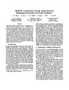
RUSH H OUR is a commercial sliding blocks puzzle. Pieces representing cars and trucks are placed on a 6 × 6 square board. The game starts by placing the vehicles according to an initial configuration as shown in Fig.1(a). The goal of the game is to get the red car to the board exit square, as shown in Fig.1(b), by moving the other vehicles out of its way. Cars and trucks take up two and three board squares, respectively. In an initial configuration, each car is positioned either vertically or horizontally and cannot steer from that direction during the game, i.e. each vehicle stays on its initial row or column, respectively. As a consequence, the target car must be facing the exit from the beginning. The commercial game provides 40 cards describing initial board configurations, with various number of cars. They are ranked in four levels: beginner, intermediate, advanced and expert. The motivation of this paper is to find the hardest initial board configurations of the game. We consider that a configuration is hard if the minimal number of moves necessary to exit the red car is high. This problem is challenging for two reasons. First, the number of possible initial configurations of the game is huge: around 3.610 configurations for 6 × 6 board. Second, finding the minimal length of a solution to a single ?

?? ??? †

Supported by the FRFC project “Centre F´ed´er´e en V´erification” funded by the Belgian National Science Fundation (FNRS) under grant nr 2.4530.02 Aspirant du F.N.R.S. CS, Universit´e Libre de Bruxelles, Belgium Department of Computer & Decision Engineering, CoDE, Universit´e Libre de Bruxelles, Belgium

6

14

5

B

A

4

E

13 A

1

RED

RED

Exit

D

15

Exit

D

3

B

C

C

b. Winning configuration

2

E

a. Initial configuration

Exit

16

18

17 24

c. Hardest initial Rush Hour configuration

Fig. 1. RUSH H OUR

initial configuration is already a hard problem. Indeed, RUSH H OUR algorithmic complexity was first studied by G. W. Flake and E. B. Baum in [1]. Their work inspired a more general sliding blocks complexity proof technique by R. A. Hearn and E. D. Demaine in [2]. These works show that the problem of deciding if an initial configuration is solvable for a generalized version of RUSH H OUR with arbitrary board size, is PS PACE -C OMPLETE. This implies that there is no polynomial time algorithm to find a solution (unless P=PS PACE) and the length of the shortest solution of hard initial configurations grows exponentially with the board size n (provided that P 6= NP and NP6= PS PACE). In this paper, we present an elegant solution to compute the hardest configurations of the RUSH H OUR game. This solution relies on the propositional modeling of the (huge) graph of configurations that underlies the game and on the implicit exploration of this graph using symbolic model-checking techniques. Symbolic model-checking techniques have been developed since the early nineties by the computer aided verification research community and have shown successful in verifying logical properties of complex hardware circuits. Symbolic model-checking techniques are useful to explore very large graphs (with 1020 states for example, see [8]) and to compute properties of the paths in those graphs. The graphs are represented implicitely using symbolic data structure such as Binary Decision Diagrams (BDDs) [4]. The contributions of this paper are the following. First, we show that symbolic model-checking techniques can be used successfully to analyze the entire configuration space of the 6 × 6 RUSH H OUR game with reasonable computational resources. Symbolic model-checking techniques allow computing the hardest configurations of the game. Second, we show that, unfortunately, the most natural way of modeling the game into propositional logic leads to the construction of symbolic data-structures whose size explodes. We prove that this phenomenon is not limited to the symbolic analysis of RUSH H OUR but will occur for any board game. Indeed, we show that the symbolic representation of simple constraints like “A position of the board can only hold one piece” requires BDDs whose size is exponential in the problem size. To avoid this phenomenon, we propose a dual modeling of RUSH H OUR which leads to more manageable symbolic data-structures. This modeling can be straigthforwardly translated into the input language of N U SMV [6], a state of the art symbolic model-checking tool. This second modeling allows to successfully apply symbolic model checking methods and to classify the entire set of configurations of the game according to the length of its minimal solution. This shows that the choice of modeling is crucial for the successful application of symbolic model checking techniques. The application of these techniques to other games, like chess or checkers, should be studied. Third, we show that the tech-

niques proposed here can not only be used to compute hard initial configurations but are also useful to analyze interesting structural properties of the game. The rest of this paper is organized as follows. In Section 2, we formalize the problem, present a general breadth first search algorithm and an estimation of the computing resources (time and memory) a classic explicit implementation would require. In Section 3, we recall the notion of Binary Decision Diagram and present a symbolic implementation of the algorithm. In Section 4, we propose a first modeling of the game into propositional logic, report on the explosion of the BDD for this modeling and we develop a theoretical argument which explains why our first modeling leads to explosion in BDD size. In Section 5, we come up with a dual modeling of the game that takes into account the theoretical result of the previous section. In Section 6, we report on the success of the second modeling and present some interesting results on the hardest initial configurations of the game.

2

Formalization of the problem

In this section, we show how the RUSH H OUR hardest configurations problem can be solved by a simple backward graph exploration equivalent to a (one-player) retrograde analysis. The possible configurations of the cars on the board define the vertices of the graph and valid moves between configurations define the edges of the graph. After presenting this conceptually simple solution, we evaluate the cost of traversing the graph of configurations with an explicit algorithm that operates at the level of vertices of the graph (treats each vertex individually). 2.1

The hardest configurations

Let G = (V, E) be a finite directed graph: V is the set of vertices and E ⊆ V × V is the set of edges. Let v ∈ V and U ⊆ V . A path from v to U is a sequence of vertices ρ = v1 v2 . . . vn such that v1 = v, vn ∈ U and ∀i·1 ≤ i < n·(vi , vi+1 ) ∈ E. The length of the path ρ = v1 v2 . . . vn , noted |ρ|, is n − 1. The set of paths from v to U in G is noted PathG (v, U ). The distance from v to U is equal to Min{|ρ| | ρ ∈ PathG (v, U )} if PathG (v, U ) is non empty and equal to +∞ otherwise, this value is noted DistG (v, U ). Let us now consider a graph, GRH = (VRH , ERH ), whose vertices represent the valid configurations of RUSH H OUR (board configurations without collision) and the edges the valid transitions between those configurations. Let us denote the set of winning configurations as W. A configuration v ∈ VRH is of index n ∈ N if DistGRH (v, W) = n. Our goal is to compute the set of configurations of the largest index n. A classical breadth first search algorithm can be applied. Starting from the set of the winning configurations, we successively compute the set of configurations of index n until reaching an empty set. The last non-empty set contains the hardest configurations of the game. In the sequel we name this algorithm retrograde analysis in analogy with the two-player game analysis method. We are now equipped to compute in GRH all the configurations that can reach a winning configurations and their index. The set of configurations of index k is noted Ck and it is computed inductively as: C0 = W; R = W; for each v ∈ (Ci−1 ) do for i > 0 for each w with (w, v) ∈ ERH and w ∈ / R do add v into Ci and into R

Note that if Ci = ∅ then Cj = ∅ for all j ≥ i. So our algorithm will start from C0 and compute the sets Ci ’s until we get an empty set. 2.2 Explicit implementation Solving this problem with classical retrograde analysis is theoretically feasible. The challenge is to deal with the huge state space: 3.6 · 1010 valid configurations. The breath first search algorithm requires in this case a mapping between each configuration and a bit telling wether or not it has been visited before. A clever indexing scheme is not enough to make the map fit into the computer’s limited memory, since it requires at least 4.5 GB (3.6 · 1010 bits). However, partitioning the problem to make it fit is straightforward. Since the vertical cars cannot leave their respective column and horizontal cars cannot steer from their respective line, the number of cars and trucks for each line is an invariant of transitions. Fixing these numbers defines a partition of our problem. We can solve each of these partitions independently of each other. These partitions do fit easily into memory. Indeed, for a line with 1 car there are 5 possible positions, with 1 truck there are 4 possible positions, for 2 cars there are 6 possible positions, for a line with 1 car followed by a truck there are 4 positions. Let consider one of these partitions and let ni be the number of possible positions for the i-th line and mi the number of possible positions for the i-th column. We have 1 ≤ ni , mi ≤ 6, thus there are at most 612 = 2 · 109 possible configurations in a partition. We need only one bit telling if the configuration has been visited or not, so we need about 2 · 109 bits of memory which is about 270 MB. A closer look at the possible configurations of a partition would show a smaller memory requirement. For example, we do not need to include in the map the winning configurations nor configurations with more than 17 cars (since the board has 36 squares). This takes care of the first obstacle: fitting the problem into the limited physical memory of a standard computer. However this is only half the solution. We broke down the problem into 612 = 2·109 subproblems since there are 6 possible configurations of a line or column (no car, 1 car, 2 cars, 1 truck, 1 car followed by a truck, 1 truck followed by a car) and there are 6 lines and 6 columns. We now must solve these subproblems. For each of these partitions we must generate the set of winning configurations. Then, for each of these winning configurations, we compute the configurations we can reach in one step, update the map accordingly and keep track of the newly reached configurations. Once all winning configurations have been treated, we apply the same operations to the set of newly reached configurations iteratively, until reaching an empty set. The tricky part that we do not tackle here is generating in an efficient manner the set of winning configurations of a partition. This method has to treat the 3.6 · 1010 configurations. According to preliminary experiments, this can be achieved in about 20 hours. This section showed that we can use a classical retrograde analysis algorithm, but it needs a significant amount of computing resources. This also gives us a rough idea of expected performance to compare our results with.

3

Symbolic Implementation

In this section, we turn the explicit algorithm of previous section, whose basic operations treat vertices individually, into a symbolic algorithm whose basic operations treat set of vertices instead. To implement such an algorithm, we need a data structure to manipulates set of configurations efficiently. We present such a data structure and then we give our symbolic algorithm.

3.1

Symbolic data structure

Reduced Ordered Binary Decision Diagrams (ROBDD), introduced by R. Bryant [4] in 1986, are data structures that canonically represent boolean functions as direct acyclic graphs. Equivalently they are canonical representation of set of valuations that can be exponentially smaller than the sets it represents. This data structure has found tremendous success in verification of the logic of hardware circuits. So ROBDD’s are natural candidates to symbolically represent the sets that we have to handle in the algorithm of next section. As an illustration, the set of valid configurations containing 3.6 · 1010 configurations is represented with a BDD containing 10 Million nodes in our second modelling (see section 5). This is 3600 configurations per node. Furthermore, as we will see, the operations are performed on the compressed representation without decompression. ROBDD’s are essentially binary decision trees where the sequence of variables associated with the nodes of any path follows a given global order and where common subtrees have been shared across the tree. They provide computation of operations with interesting complexity. More precisely, a binary decision diagram, or BDD, is a rooted acyclic graph with two terminal nodes of out-degree zero labeled 0 or 1 and a set of variable nodes of out-degree two. This is illustrated in Figure 2 where the dotted lines represent the low branches, i.e. variable is 0, while the solid lines represent the high branches. A BDD is ordered, OBDD, if for any path the sequence of variables associated with the nodes of this path follows a given global order. A BDD node is not unique if another of its nodes has the same variable name and low and high successors. Moreover we say that a BDD node is a redundant test if it has identical low and high successors. Finally an OBDD is said to be reduced, ROBDD, if all its nodes are unique and are not redundant tests.

x

y

y

z

0

x

y

z

y

y

z

=> 1

x

0

z

=> 1

0

1

Fig. 2. BDD for the formula z ∧ (x ∨ y). Removal of non-unique node followed by removal of redundant test. The rightmost BDD is the canonical ROBDD for the ordering x < y < z, both leftmost are OBDDs.

Low complexities of important operations is what makes ROBDD’s attractive for verification methods and our problem. The central property of ROBDD’s is that, given a variable ordering, they canonically represent Boolean functions. As a consequence tautology, satisfiability and equivalence are done in constant time. Let A and B be two BDDs, |A| and |B| are their respective size, i.e. their number of nodes. Reduction algorithms run in O(|A|). Exhibiting a value that satisfies the function can be done in O(n) , where n is the number of variables. The SAT-count algorithm must output the number of assignments that satisfy the function, it has a running time of O(|A|). Union and intersection (conjunction and disjunction) algorithms have running time of O(|A| ·

|B|). The complement implemented with a tree traversal has a running time of O(|A|). Universal and existential quantification are done in O(|A|2 ). Finally the Pre operator, extensively used in verification techniques, consists of n existential quantification and thus has a running time of O(|A|2n ), diverse methods have been developed to make it as efficient as possible [5]. The complexity of the operations described above depends on the size of the BDD which may be exponentially smaller than the set it represents, but it may also vary between a linear and an exponential range depending on the ordering of the variables. It is therefore crucial to find a good ordering. However, finding the optimal ordering or even improving it has been proved to be a NP-C OMPLETE problem. Thus efficient heuristics have been studied to tackle this problem. While BDD have been introduced for Boolean formulas, this structure can easily be extended to finite integer domains through a Boolean encoding of the bounded integer variables. For efficiency reasons, the Boolean variables that encode an integer variable will be gathered in the variables ordering of the BDD. In the following, we will use BDD over finite integer domain, since it is the structure used in N U SMVand other verification tools, and when considering x we will directly refer to that variable in the BDD and not to the binary variables that encode it. 3.2

Symbolic algorithm

Let GRH = (VRH , ERH ) be the graph of the game defined above, and let X = {x1 , . . . , xk } be a set of bounded integer variables representing the system (e.g. the position and direction of each car). To each vertex of GRH corresponds a valuation of these variables. To a valuation may correspond a vertex of GRH , provided the valuation defines a valid configuration. Given a propositional formula φ, we note [[φ]] the set of valuations that satisfy φ. For example, if φ ≡ x1 ⇒ x2 , then [[φ]] is the set of valuations that maps the pair (x1 , x2 ) to a pair in {(0, 0), (0, 1), (1, 1)}. A propositional formula φ over the variables x1 , . . . , xk defines (via the set [[φ]]) a set of vertices or, equivalently, a set of configurations of the game. For any set of configurations, U ⊆ VRH , considered as a set of valuations, there is a propositional formula φU such that U =[[φU ]]. We note φW the proposition defining the winning configurations. In the same way if X 0 = {x01 , . . . , x0k } is a set of variables representing the game configuration after one transition, there is a propositional formula, φE over {x1 , . . . , xk , x01 , . . . , x0k } such that ERH =[[φE ]]. Given a set U of vertices in GRH , we define the set of one-step predecessors of U as Pre(U ) = {v ∈ VRH |∃u ∈ U : (v, u) ∈ ERH }

(1)

If U is defined by propositional formula φ over X 0 , i.e. U =[[φ(X 0 )]], then Pre(U ) is represented by the following propositional formula1 over X: ∃X 0 : φE (X, X 0 ) ∧ φ(X 0 )

(2)

Pre([[φ(X 0 )]]) =[[∃X 0 : φE (X, X 0 ) ∧ φ(X 0 )]]

(3)

So we have:

1

The existential quantification is a shorthand for the disjunction over all variables over all their finite set of possible values.

We can now symbolically apply the following algorithm: C0 =[[φW ]] Ci = Pre(Ci−1 ) \

[

Cj

for i > 0

(4)

0≤j≤i−1

All these sets can be represented by BDDs and all these operations can be directly applied on these BDDs.

4

First propositional model

We present in this section a first modeling of RUSH H OUR in propositional logic: we define φW and φE . We show that this first solution is not satisfactory and we give a mathematical argument that explains the phenomenon. This mathematical argument is general and has applications in the study of the symbolic analysis of other board games. 4.1

Formalization

Let n and m be two fixed parameters of the specification, n being the size of the board and m the number of cars. For the sake of readability, we make here the hypothesis that all vehicles have a length of 2, the modeling for vehicles of length 2 and 3 can be obtained from this one in straigthforward manner. Let the pair of variables (xi , yi ) denote the cartesian coordinates of the upper-left square occupied by the i-th car, (1, 1) being the lower-left corner of the board. Let the variable hi indicate the orientation of the vehicle, i.e. hi is 1 if the i-th car is horizontal and 0 if it is vertical. The target car uses index 1. We note X = {x1 , y1 , h1 , ..., xm , ym , hm } the set of the system variables 0 and X 0 = {x01 , y10 , h01 , ..., x0m , ym , h0m } the set of variables describing the configuration after one transition, this will be useful to specify the evolution of the system. The set of all possible configurations is S = ({1, . . . , n}2 × {0, 1})m . We specify 3 relations on S: the invariant of the system Invar ⊆ S, which denotes the legal configurations, the transition relation between configurations T rans ⊆ S × S, which does not check collision and W in ⊆ S the set of configuration with the target car on the exit square. We have: φW (X) = W in(X) ∧ Invar(X) and φE (X, X 0 ) = T rans(X, X 0 ) ∧ Invar(X 0 ) To specify those relations we use propositional formulas over finite integer domains. Invariant Proposition (5) states that cars are fully on the board, (6) states that cars do not overlap. The Invar relation is the conjunction of (5) and (6). [[Invar]] is the set of all valid states. ^ (hi < xi + hi ≤ n) ∧ ((1 − hi ) < yi ≤ n) (5) 1≤i≤m

^

(xi > xj +hj ) ∨ (xj > xi +hi ) ∨ (yi > yj +(1−hj )) ∨ (yj > yi +(1−hi )) (6)

1≤i,j≤m i6=j

In the same manner, we have propositional formulas for the set of winning configurations and for the transition relation. We omit them here, but we will give another complete formalization of RUSH H OUR in section 5. Having formalized the RUSH H OUR rules in such a way that for any couple (m, n) we obtain a Boolean propositional specification that describes the game, we can apply our algorithm.

# cars 4x4 5x5 6x6 2 123 233 368 3 1237 3918 9490 4 7334 44209 172583 5 24227 321114 2153132 6 44209 1520760 N/A 7 50081 N/A N/A 8 30762 N/A N/A 9 1 N/A N/A Table 1. Number of nodes in the Invar BDD relatively to board sizes and number of cars.

4.2

Results of first implementation

We ran our specification for board sizes n ranging from 4 to 6. For each board size the number of cars m ranged from 2 to the maximum our system memory could handle. As the number of cars increases the Invar BDD size explodes. This can be observed in table 1. We only report on the Invar BDD, since the W in and T rans BDD sizes do not explode and are thus not relevant here. The explosion in the memory consumption limited us to the exploration of boards of sizes 5 and 6, with a number of cars smaller than 6 and 5 respectively. More complex systems cannot be handled with this approach. It is a fundamental BDD property that its size increases with the number of intervariable dependencies. This is the reason why the Invar BDD size explodes. As mentioned above, the purpose of this BDD is to validate car positions against collisions. This puts in interdependency all car positions, since each car position must be checked against all others. This first negative experiments motivates the next section where we show that board games are intrinsically difficult to model with ROBDD’s. 4.3

Limitation of ROBDD-based methods for board games

In this section, we abstract the collision problem to linear boards filled with tokens. We exhibit a lower bound on the size of the ROBDD that detects a collision on this linear board. We obtain a two-dimension result as a direct corollary. An assignment of a set of tokens modelled by variables in X = {x1 , . . . , xm } on the board of size n is a function v : {x1 , . . . , xm } → {1, . . . , n}. There is no collision iff this function is injective. This is formalized by this propositional formula over finite integer domain: φcoll =

^

i 6= j → (xi 6= xj )

(7)

1≤i,j≤m

Lower bound results for ROBDDs are generally based on the concept of fooling set. Fooling sets were introduced by Sedgewick for VLSI and then applied by Bryant to ROBDD [3]. We adapt this notion here for finite integer domains. Let X = {x1 , . . . , xm } be the set of variables whose domain of values is {1, . . . , n}. Definition 1. An input assignment is a function v : X → {1, . . . , n}. Given (L, R) a partition of X. We call a left (right) input assignment any function l : L → {1, . . . , n}

(r : R → {1, . . . , n}). We denote by l · r the input assignment defined by l and r on X. We say that an OBDD is compatible with a partition (L, R) iff all variables of L precede all variables of R in this OBDD variable ordering. Before defining the notion of fooling set, we need an additional notion. Let V = {v | v : X → {1, . . . , n}} be the set of valuations for variables in X. A function f : V → {0, 1} partitions the valuations as making the function true or false. We compactly note the type of such a function by f : [X → {1, . . . , n}] → {0, 1}. Definition 2. Let (L, R) be a partition of X and f be a function such that f : [X → {1, . . . , n}] → {0, 1}. A fooling set F for f over L is a set of left assignments such that: for any l, l0 ∈ F, l 6= l0 , there exists a right assignment r with f (l · r) 6= f (l0 · r). Such a right assignment is said to distinguish between l and l0 . Lemma 1. Given a partition (L, R) over X, a function f : [X → {1, . . . , n}] → {0, 1} and a fooling set F for f over L, then any OBDD compatible with (L,R) has more than #F nodes. Proof. For any two distinct left assignments, l and l0 , of F there exists, by definition of F , a right assignment r that distinguish them, i.e. such that f (l ·r) = 0 and f (l0 ·r) = 1. It follows that l and l0 must lead to two different “intermediate” nodes in the OBDD and thus that there is at least as many nodes as there are elements in F . We now prove a lower bound on the size of any OBDD that detects the collision of tokens on a linear board. Theorem 1. Let f : [X → {1, . . . , n}] → {0, 1} such that f (v) = 1 iff v |= φcoll , where φcoll is defined in (7). Let A be an ROBDD over the set of variables X = {x1 , x2 , . . . , xm } representing f . A has at least Cnm−1 nodes. Proof. Let N be the set of subsets of m − 1 values from {1, . . . , n} and let X1 = {x1 , . . . , xm−1 } and X2 = {xm }. To each N ∈ N we associate one bijection fN : X1 → N . We note F this set of functions. F is a fooling set for f over X1 : let l1 , l2 ∈ F with l1 6= l2 . By construction of F, we know that codom(l1 ) 6= codom(l2 ), and let n1 be a value such that n1 ∈ codom(l1 ) and n1 ∈ / codom(l2 ). Let r : X2 → {1, . . . , n} be an injective function such that codom(r) ∩ codom(l1 ) = n1 and codom(r) ∩ codom(l2 ) = φ. We have f (l1 · r) = 0 and f (l2 · r) = 1. Applying lemma 1 finishes the proof since N has Cnm−1 elements. Since a two-dimension board is equivalent to a linear board with n2 squares, we have as a corollary: Corollary 1. Let A be a BDD over the position variables X = {x1 , y1 , x2 , y2 , ..., xm , ym } for a two-dimension board of size n with m tokens. If, for every 1 ≤ i ≤ m the variables {xi , yi } are gathered in the BDD variable ordering, then A has at least Cnm−1 nodes. 2 Note that this result is fundamentally connected to the chosen encoding of the problem. The token positions are encoded in a cartesian-like board coordinates style. Applying this result to board games we obtain a lower bound on any ROBDD representing the collision of pieces on a chess board or on draughts board with the afore mentioned encoding. The lower bounds in table 2 suggests this technique is not suitable to explore chess and droughts with more than 5 to 6 pieces (additional complexity will be brought in with the complex rules of these games).

# of pieces Chess Draughts American checkers RUSH H OUR Invar BDD size (observed) 2 64 49 32 368 3 2.016 1176 496 9.490 4 41.664 18.424 4960 172.583 5 635.380 211.876 35.960 2,1M 6 7.6M 1.9M 201.376 N/A 7 75M 14M 906.192 N/A 8 620M 86M 3.4M N/A Table 2. Lower bounds on the size of the ROBDDs detecting pieces collisions for chess, draughts and american checkers board.

A dual encoding is to use a boolean variable for every square of the board that indicates if the square is occupied or not. For board games with more complex tokens, like american checkers or chess, an integer, that indicates which kind of pieces occupied the board if one, is required. Using this dual encoding, Baldamus et al. explored the possibility to solve american checkers with ROBDD[7]. They observed an explosion in the size of ROBDD preventing them to solve american checkers for boards with size greater than 4 × 4. American checkers is the simplest game considered here. However, the number of legal positions is estimated to be 1018 .

5

Dual propositional model

In the light of the previous section, we propose now a dual encoding of the RUSH H OUR board which limits the explosion of the size of the symbolic structure. Because vehicles take more than one square, we work on a line and column level, instead of on a square level as in [7]. We have shown that interdependencies between the variables lead to huge ROBDDs. Here, we try to limit these interdependencies using a specific property of RUSH H OUR: two horizontal cars on different lines can never collide. Similarly, vertical cars cannot collide with other vertical cars that are not on the same column. This is the basic idea behind our second model. Again, for the sake of readability, the model below is limited to vehicle of size 2. Our actual implementation is general, it takes into account vehicles of size 2 and 3. Let n be the size of the board. On each column and each line we have at most k = bn/2c cars. Let hi,j = (ohi,j , phi,j ), 1 ≤ i ≤ n and 1 ≤ j ≤ k represents the j-th horizontal car of the i-th row, such that this car is on the board if ohi,j = 1 and out of the board if ohi,j = 0. If on the board, its leftmost square is on the phi,j square (from the left) of the i-th row. Similarly, let vi,j = (ovi,j , pvi,j ) , 1 ≤ i ≤ n and 1 ≤ j ≤ k represents the j-th vertical car of the i-th column, such that this car is on the board if ovi,j = 1 and out of the board if ovi,j = 0 and its upper square is on the pvi,j square (starting from the 0h v v bottom) of the i-th column. We have 0 ≤ pvi,j , pvi,j < n. Let (o0h i,j , pi,j ) and (oi,j , pi,j ), for 1 ≤ i ≤ n and 1 ≤ j ≤ k, describe the configuration after a transition. Invariant Proposition (8) states that cars on the same line, column, do not overlap and (9) that any horizontal car does not collide with any vertical car. The Invar relation is the conjunction of (8) and (9).

^

(odi,j = 1 ∧ odi,j 0 = 1 ∧ j < j 0 ) → pdi,j < pdi,j 0 − 1

(8)

 (ohi,j = 1 ∧ ovi0 ,j 0 = 1)  →
0 h 0 v v ≤ i − 2) ∨ (pi,j > i ) ∨ (pi0 ,j 0 ≤ i − 2) ∨ (pi0 ,j 0 > i)

(9)

d∈{h,v} 1≤i≤n,1≤j,j 0 ≤k

 ^  0

1≤i,i ≤n 1≤j,j 0 ≤k

(phi,j

Transition Proposition (10) states that only one car is moving during one transition. Proposition (11) states that vehicles on the board stay on the board, and vehicles out of the board stay out of the board. Finally, proposition (12) states that cars move one square at a time. The transition relation is the conjunction of these propositions: ^ d0 0d0 (10) pdi,j 6= p0d i,j → pi0 ,j 0 = pi0 ,j 0 d,d0 ∈{h,v} 1≤i,i0 ≤n,1≤j,j 0 ≤k

^

odi,j = o0d i,j

(11)

|pdi,j − p0d i,j | ≤ 1

(12)

d∈{h,v} 1≤i≤n,1≤j≤k

^ d∈{h,v} 1≤i≤n,1≤j≤k

Winning configuration One of the car of the exit square row is on the board and positioned on the exit square. Let e be the number of the exit square row, we have: _ [(pde,j = n − 1) ∧ (ode,j = 1)] 1≤j≤k

6

Results: RUSH H OUR hardest configuration

Contrary to the first encoding, the second encoding gives rise to manageable symbolic data-structures. Using N U SMV, we were able to analyze the entire configuration space of RUSH H OUR . Here are some representative results of our analysis. Hardest configuration The hardest configuration of the RUSH H OUR game is given in Figure 1c and it requires 93 steps to reach a winning configuration. From that initial configuration 24132 configurations can be reached. This gives a good idea of the difficulty of this configuration: please give it a try. Besides finding the hardest configuration, our analysis has classified every solvable according to the length of its minimal solution. Table 3 presents the number of configurations for the greatest indexes. We learn there are 1010 winning configurations and 2.98·1010 solvable configurations, thus, about 7 billions of valid configurations have no solution, while about 19 billion non-winning configurations have one. The vast majority of the latter are very easy (shortest solution is very short). Our symbolic solution can also be used to isolate, what we think are, the most interesting configurations of the game. We say that one configuration dominates another

Index 93 92 91 90 89 88 87 86 85 # configurations 1 6 14 26 47 80 123 172 223 # dominating configurations 1 0 0 2 2 2 1 3 6 Table 3. Number of configurations in the furthest frontiers

if the latter is reachable from the former and the index of the former is greater than the index of the latter. We present in Table 3 for each index the number of configurations that are not dominated. Performance The results were obtained on an Intel(R) Xeon(TM) CPU 3.06GHz and our symbolic algorithm used up to 1.5GB. It took about 10 hours to complete the total exploration of RUSH H OUR . Since there are about 3.6 · 1010 valid configurations this is about 106 configurations each second. While the running time is comparable to the explicit implementation shown in section 2.2, we stress that the symbolic method is more generic (standard data structure, generic algorithms), while the explicit implementation had to be conceived for the RUSH H OUR game. Moreover, at the end of the computation, we keep the whole structure in memory. This allows us to perform various kinds of queries easily, for instance we can retrieve all hard configurations without trucks, with exactly 3 cars, etc. These results should encourage to study more deeply the application of symbolic methods to other games such as chess or checkers.

References 1. G. W. Flake and E. B. Baum, RUSH H OUR is PSPACE-complete, or Why you should generously tip parking lot attendants , in Theoretical Computer Science, 270(1-2), 895-911, 2002. 2. R. A. Hearn and E. D. Demaine, PSPACE-Completeness of Sliding-Block Puzzles and Other Problems through the Nondeterministic Constraint Logic Model of Computation, to appear in 2004. http://arxiv.org/abs/cs.CC/0205005 3. R. E. Bryant, On the Complexity of VLSI Implementations and Graph Representations of Boolean Functions with Application to Integer Multiplication, in IEEE Transactions on Computers 40(2), 205-213, 1991. 4. R.E. Bryant. Graph-based Algorithms for Boolean Function Manipulation, IEEE Trans. Comput., C-35(8), 1986. 5. C. Meinel, T. TheobaldAlgorithms and Data Structures in VLSI Design: OBDD - Foundations and Applications, Springer-Verlag, 1998. 6. A. Cimatti et al, NuSMV 2: An OpenSource Tool for Symbolic Model Checking, In Proceeding of International Conference on Computer-Aided Verification, 2002. 7. M. Baldamus, Can American Checkers be Solved by Means of Symbolic Model Checking?, in Workshop on Formal Methods Elsewhere, Pisa, Italy, 2000. 8. J. R. Burch et al., Symbolic Model Checking: 1020 States and Beyond, in Proceedings of the Fifth Annual IEEE Symposium on Logic in Computer Science, 1-33, 1990. 9. G. J. Holzmann, SPIN Model Checker, The: Primer and Reference Manual, Addison Wesley Professional, 2004.