From: AAAI-98 Proceedings. Copyright © 1998, AAAI (www.aaai.org). All rights reserved.
On the Computation of Local Interchangeability in Discrete Constraint Satisfaction Problems Berthe Y. Choueiry Knowledge Systems Laboratory Stanford University Stanford, CA, 94305-9020
[email protected]
Abstract In [4], Freuderdefines several types of interchangeability to capture the equivalenceamongthe values of a variable in a discrete constraint satisfaction problem (CSP), and provides a procedure for computing one type of local interchangeability.In this paper, we first extend this procedurefor computinga weakform of local interchangeability. Second,weshowthat the modifiedprocedurecan be used to generate a conjunctive decompositionof the CSPby localizing, in the CSP,independentsubproblems.Third, for the case of constraints of mutualexclusion, we showthat locally interchangeablevalues can be computedin a straightforward manner, and that the only possible type of local interchangeabilityis the onethat induceslocally independent subproblems. Finally, we give hints on howto exploit these results in practice, establish a lattice that relates sometypes of interchangeability, and identify directions for future research. 1 Introduction Interchangeability amongthe values of a variable in a Constraint Satisfaction Problem(CSP) captures the idea of ’equivalence’ amongthese values and was first formalized by Freuder [4]. Choueiry and Faltings [2] showthat interchangeability sets are abstractions of the CSPwith the following advantages: 1. The reduction of the computational complexity of a problem, and the improvement of the performance of the search technique used to solve it. 2. The identification of elementary componentsfor interaction with the users. This paper studies the computation of local interchangeability, and is organized as follows. In Section 2, we first review the definitions of a CSPand interchangeability; we discuss the advantages drawn from computing interchangeable sets; then we restate the procedure introduced in [4] for computinga strong type of local interchangeability. In the rest of the paper we describe our contributions. In Section 3.1, we extend the above mentioned procedure; we show that this extension enables the computation of a weak form of interchangeability (Section 3.2) as well as the
Guevara Noubir Data Communications Group Centre Suisse d’Electronique et de Microtechnique (CSEM), Rue Jaquet-Droz CH-2007Neuch~tel, Switzerland
[email protected]
identification of locally independent subproblems(Section 3.3); then we describe howthese interchangeable sets are organized in a hierarchy (Section 3.4). Further, we sketch howto use their properties in practice (Section 4), and showthat, for the case of constraints of mutual exclusion, local interchangeability can be easily computed, and is equivalent to identifying locally independent subproblems (Section 5). Finally, we introduce a lattice that situates various contributions reported in the literature (Section 6), and draw directions for future research (Section 7). Weintentionally restrict ourselves here to presenting the concepts, hinting on their usefulness, and illustrating them on simple problems. Although we have already identified several properties useful for problem solving, we do not discuss them here for lack of space. 2 Definitions A CSP is defined by 7~ -- (]),7),C), where {V1,V2,...,Vn} is the set of variables, 7:) {Dv1,Dv2,...,Dv~) the set of domains (i.e., sets of values) associated with the variables, and C is the set of constraints that apply to the variables. A constraint Cv,~, applicable to two variables V~ and Vj, restricts the combination of values that can be assigned simultaneously to ~ and Vj, and thus defines a relation Rv~,v~ C_ Dv~× Dvj, which is the set of tuples allowed by Cv,½.. Whenthe relation is exactly the Cartesian product of the variable domains (i.e., R~,D -- DR x DR), the corresponding constraint is said to be universal. To solve a CSPis to assign one value to each variable such that all constraints are simultaneously satisfied. A CSPis commonlyrepresented by a constraint graph in which the variables are represented by nodes, the domains by node labels, and the constraints by edges that link the relevant nodes. Universal constraints are omitted from the constraint graph. In this document,we restrict our study to discrete binary CSPs: each domain Dt~ is a finite set of discrete values, and each constraint applies to two variables. Wedefine the neighborhoodof a set of variables S, denoted Neigh(S), to be the set of variables adjacent to S in the constraint graph.
2.1 Interchangeability Freuder introduces several types of value interchangeability for a CSPvariable. Below, we recall those relevant to our study, while illustrating each of them on the list coloring problemof Fig. 1.
Figure 1: Anexampleof a list coloring problem. Definition 2.1 Full interchangeability: A value b for a CSPvariable Vi is fully interchangeable (FI) with a value c for 1,~ if and only if every solution to the CSPthat assigns b to II/remains a solution when c is substituted for b in II/and vice versa. TwoFI values b and c can be switched for variable ~ in any solution regardless of the constraints that apply to Vi. In Fig. 1, d, e, and f are fully interchangeable for 1/4. Indeed, we inevitably have 112 = d, which implies that 111 cannot be assigned d in any consistent global solution. Consequently, the values d, e, and f can be freely permutedfor 114 in any global solution. Noefficient general algorithm for computing FI has to date been reported: in fact, determining FI may require computing all solutions. Neighborhood interchangeability (NI) only considers local interactions, and can thus be efficiently computed: Definition 2.2 Neighborhood interchangeability: A value b for a CSPvariable If/ is neighborhoodinterchangeable(NI) with a value c for Vi if and only if for every constraint C on Vi: {x I (b, x) satisfies C} = {x I (c, x) satisfies In Fig. 1, e and f are NI for II4. NI and FI are special cases of k-interchangeability, which introduces gradually levels of full interchangeability in all subproblems of size k, movingfrom NI for k = 2 (local), towards FI for k = n (global). k-interchangeability (including FI and NI) is concerned with changing values of one variable, while keeping those of all other variables unchanged. Another type of interchaageability introducedin [4], partial interchangeability, allows a subset of the variables (,4 C_ )2) to be affected whenswitching the values of ~, while the rest of the ’world’ (l)-Vi--4) remains the same. Informally, partial interchangeability is about extending a boundary (which is the set of variables S affected by the switching operation) by weakening the requirement on what may be affected. Definition 2.3 Partial Interchangeability: Twovalues are partially interchangeable (PI) with respect a subset .4 of variables if and only if any solution involving one implies a solution involving the other, with possibly different values for variables in .4.
In Fig. 1, a and b are PI for V1with respect to the set .4 = {113}. There is no knownefficient algorithm for computingthe H-sets for a CSPvariable. In addition to the difficulty of computing PI, one also needs to specify the set .4, which is not a straightforward task. In this paper, we extend the polynomial algorithm for computingNI to efficiently computea localized version of PI, whichwe call NPIand define in Section 3.2. Notice that FI corresponds to PI with .4 = ~; and similarly, NI corresponds to NPI with .4 = ~. Fig. 2 illustrates the relations between these types of interchangeability (from local to full, and from strong to weak). Informally, a variable V~ affects the problem extenffmg the bound FI ~ enforcingconsistency ~ NI ~
PI
o v, ~ ,,’~)Boundary NPI 0 csPvariable
strong weak local Figure 2: Interchangeability. Partial (-,~): fromstrong weak.Full (=~): from local to global. ’through’ the constraints that link 1I/to other variables in the problem, thus through Vi’s neighborhood. Two values x and y that are NI for 11/’affect’ Neigh({Vi}) exactly the same fashion. They are bound to carry the same effect on the whole problem, and are inevitably FI for V~. More formally, Freuder shows that NI is a sufficient but not a necessary condition for FI. (Indeed, in the exampleof Fig. 1, d and e for 114 are FI but not NI.) It is easy to show that the same relation holds between NPI and PI. Weintroduce the relation -c that links values x and y, variables 11/ and Vj in S C )d, and the constraints g of the CSPto indicate that the variable-value pairs (Vi, x) and (Vj, y) are compatible with exactly the variable-value pairs in Neigh(S). (x, V/, S) -=e (Y, Vj, S) If x and y are NI for V/, we have (x, V/, {1I/}) (y, 11/, {II/}); if they are PI, wehave(x, V/, {V/}U-4) (y, 11/, {Vi} U .4). This relation is symmetricand transitive, becauseit is in essence a relation of equivalence. 2.2 Advantages of interchangeable values Weidentify three main ways to use interchangeable values in practice: 1. Strongly interchangeable values can be replaced by one ’meta-value’. 2. An asymmetric type of interchangeability, called substitutability (see Definition 5.4), can be used accommodateunquantifiable constraints or subjective preferences. 3. Partial interchangeability localizes the effect of modifications to somevariables and identifies compact
families of partial solutions: qualitatively equivalent solutions can be generated by modifying the values of the indicated variables only. Classical enumerative methodsfail to organize the solution space in such a compact manner: they present solutions in a jumble without showingsimilarities and differences betweenalternative solutions. In particular, they fail to identify the boundaries within which the effect of a changeremains local. In practice, these characteristics can be used as follows, beyond and including search: In interactive problem solving. Interchangeable sets can be used to help the humandecision-maker view alternative choices in a concise way [2]. More specifically, meta-values can be used to avoid displaying too much information to the user; substitutability allows the compliance to users’ preferences; and finally, partial interchangeabilities delimit the extent of certain modifications, so that the users can modifya solution locally to cope with change in a dynamic environment. In search. Interchangeability sets can be used (1) monitor the search process to remain as local as possible, by compactingthe solution space representation and by grouping solution families, and (2) enhance the performance of both backtracking and consistency checking by removing redundant values, as shownin [1; 7]. In explanation. Interchangeability identifies groups of objects (sets of variables and sets of values) becomethe basic components for a concept generation process aimedat providing explanation. In realworld applications, it is reasonable to suspect that the set of objects discovered to be interchangeable share commoncharacteristics [4]. In [2], a concept generation procedure uses background knowledge, in the form of concept hierarchies, to generate dynamically concise descriptions of the interchangeable sets. 2.3 The discrimination tree Below, we recall the procedure, introduced in [4], for computing the NLsets for a variable by building its discrimination tree (DT). The complexity of this procedure is O(nd2), where n is the size of )2, and d the size of the largest domain. It is important, in this procedure, that variables and values be ordered in a canonical way. Algorithm 1 DT for Vi (nvi,Neigh({l~})) Create the root of the discriminationtree Repeatfor each value v 6 Dvi: Repeatfor each variable Vj E geigh({P~}): Repeatfor each w 6 Dv~consistent with v for V~: Moveto if present, construct and moveto if not, a child nodein the tree corresponding to ’Vj --- w’. Add’~, {v}’ to annotation of the node(or root), Gobackto the root of the discriminationtree.
The collection of the annotationsin the discriminationtree of a variable Vi yields the followingset: DT(~)={dll, d21,. ¯ ¯, dki} (2) where 1 < k < IDyll is the number of annotations in the tree, and dli, d2i,.. ¯, dki determinea partition of D~. The NI-sets of Vi are expressed as follows: NI(P~) = {dk~ 6 DT(V/) such that [dki[ > 1} (3) Although this was not explicitly stated in [4] or in other papers on this topic, there may be in general any numberof NI-sets per variable. In Fig. 3, we show the graph and constraints of a simple CSP. The annoDiscdmination tre~ for VI V1
vl
~
vl