ON THE CONTROL OF ASYNCHRONOUS MACHINES WITH ... - Fcla

ON THE CONTROL OF ASYNCHRONOUS MACHINES WITH INFINITE CYCLES

By NIRANJAN VENKATRAMAN

A DISSERTATION PRESENTED TO THE GRADUATE SCHOOL OF THE UNIVERSITY OF FLORIDA IN PARTIAL FULFILLMENT OF THE REQUIREMENTS FOR THE DEGREE OF DOCTOR OF PHILOSOPHY UNIVERSITY OF FLORIDA 2004

Copyright 2004 by Niranjan Venkatraman

To my parents, who always stood by me.

ACKNOWLEDGMENTS First and foremost, I would like to acknowledge the unflagging support and excellent supervision of my advisor, Dr. Jacob Hammer, during my four years at the University of Florida. I thank Dr. Haniph Latchman, Dr. Tan Wong, and Dr. John Schueller for all their efforts and their advice, and for serving on my Ph.D. supervisory committee. I would like to especially thank Xiaojun Geng (my officemate for three years) for our animated and interesting discussions. I also extend special thanks to my current officemates (Jun Peng and Debraj Chakraborty) for making the last year interesting and full of fun. Special thanks are also due to my roommates (Raj, Nand and Arun) for putting up with my eccentric behavior for four years. I would also like to thank all my friends; their unceasing friendship and care has made this work possible. Last but not the least, I would like to thank my parents, my grandmother, my sister, her husband and my other relatives for their unfailing love and support during all the years that I have been away from them.

iv

TABLE OF CONTENTS page ACKNOWLEDGMENTS ................................................................................................. iv LIST OF TABLES............................................................................................................. vi LIST OF FIGURES .......................................................................................................... vii ABSTRACT..................................................................................................................... viii CHAPTER 1

INTRODUCTION ........................................................................................................1

2

TERMINOLOGY AND BACKGROUND ................................................................10 2.1 2.2

3

Asynchronous Machines and States .................................................................10 Modes of Operation ..........................................................................................14

INFINITE CYCLES ...................................................................................................20 3.1 3.2 3.3 3.4 3.5 3.6

Introduction.......................................................................................................20 Detection of Cycles...........................................................................................22 Stable State Representations for Machines with Cycles...................................29 Stable Reachability ...........................................................................................32 Matrix of Stable Transitions and the Skeleton Matrix......................................34 Corrective Controllers ......................................................................................39

4

THE MODEL MATCHING PROBLEM...................................................................46

5

EXAMPLE .................................................................................................................59

6

SUMMARY AND FUTURE WORK ........................................................................65

LIST OF REFERENCES...................................................................................................68 BIOGRAPHICAL SKETCH .............................................................................................76

v

LIST OF TABLES Table

page

5-1. Transition table for the machine Σ. ...........................................................................59 5-2. Stable transition table for the generalized stable state machine Σ|s ..........................60 5-3. Matrix of one-step generalized stable transitions R(Σ|s) ...........................................60 5-4. Stable transition function of the given model Σ′. ......................................................61

vi

LIST OF FIGURES Figure

page

1-1. Control configuration for the asynchronous sequential machine Σ.............................3

vii

Abstract of Dissertation Presented to the Graduate School of the University of Florida in Partial Fulfillment of the Requirements for the Degree of Doctor of Philosophy ON THE CONTROL OF ASYNCHRONOUS MACHINES WITH INFINITE CYCLES By Niranjan Venkatraman August 2004 Chair: Jacob Hammer Major Department: Electrical and Computer Engineering My study deals with the problem of eliminating the effects of infinite cycles on asynchronous sequential machines by using state feedback controllers. In addition to eliminating the effects of infinite cycles, the controllers also transform the machine to match the behavior of a prescribed model. My study addresses machines in which the state is provided as the output of the machine (input/state machines). Algorithms are provided for detecting infinite cycles in a given machine, for verifying the existence of controllers that eliminate the effects of infinite cycles, and for constructing the controllers whenever they exist. The feedback controllers developed in my study resolve the model matching problem for machines that are afflicted by infinite cycles. They transform the given machine into a machine whose input/output behavior is deterministic and conforms with the behavior of a prescribed model. Thus, the feedback control strategy overcomes the

viii

effects of infinite cycles as well as any other undesirable aspects of the machine’s behavior. Results include necessary and sufficient conditions for the existence of controllers, as well as algorithms for their construction whenever they exist. These conditions are presented in terms of a matrix inequality. The occurrence of infinite cycles produces undesirable behavior of afflicted asynchronous sequential machines. The occurrence of hazards has been a major problem since the early development of asynchronous sequential machines. There are many methods to design cycle-free machines; but the literature does not seem to contain any technique for eliminating the negative effects of infinite cycles in case it occurs in existing asynchronous sequential machines.

ix

CHAPTER 1 INTRODUCTION Asynchronous sequential machines are digital logic circuits that function without a governing clock. They are also described variously as clockless logic circuits, self-timing logic circuits, and asynchronous finite state machines (AFSMs). Asynchronous operation has long been an active area of research (e.g., Huffman 1954a, 1954b, 1957), because of its inherent advantages over commonly used synchronous machines. One of the more obvious advantages is the complete elimination of clock skew problems, because of the absence of clocks. This implies that skew in synchronization signals can be tolerated. The various components of the machine can also be constructed in a modular fashion, and reused, as there are no difficulties that are associated with synchronizing clocks. Further, the speed of the circuit is allowed to change dynamically to the maximal respond speed of the components. This leads to improved performance of the machine. Asynchronous machines are by nature adaptive to all variations, and only speed up or slow down as necessary (Cole and Zajicek (1990), Lavagno et al. (1991), Moon et al. (1991), Yu and Subrahmanyam (1992), Fisher and Wu (1993), Furber (1993), Nowick (1993), Nowick and Coates (1994), Hauck (1995)). Asynchronous machines also require lower power, because of the absence of clock buffers and clock drivers that are normally required to reduce clock skew. The switching activity within the machine is uncorrelated, leading to a distributed electromagnetic noise spectrum and a lower average peak value. Moreover, asynchronous operation is inherent in parallel computation systems (Nishimura (1990), Plateau and Atif (1991), Bruschi et al. (1994)). 1

2 Asynchronous design is essential to ensure maximum efficiency in parallel computation (Cole and Zajicek (1990), Higham and Schenk (1992), Nishimura (1995)). Asynchronous machines are driven by changes of the input character, and are selftimed. In this context, it is vital to address design issues, especially those that can lead to potential inconsistencies in the pulses that propagate through the machine. These difficulties are referred to as “hazards” (Kohavi (1970), Unger (1995)). A cycle is one such potential hazard in the operation of asynchronous machines. It causes the machine to “hang,” as is demonstrated in software applications with coding defects that can cause the program to hang in an infinite loop. A “critical race” is another hazard that causes the machine to exhibit unpredictable behavior. These hazards can occur because of malfunctions, design flaws, or implementation flaws. The common procedure followed when a hazard occurs is to replace the machine with a new one, built with no defects. In our study, we propose to employ control techniques to devise methods that take a machine out of an infinite cycle and endow it with desirable behavior. Thus, we concentrate on the design of controllers that resolve infinite cycles and control the machine so as to achieve specified performance. To explain the mode of action of our controllers, a basic description of the structure of an asynchronous machine needs to be reviewed. An asynchronous machine has two types of states: stable states and unstable states. A stable state is one in which the machine may linger indefinitely, while an unstable state is just transitory, and the machine cannot linger at it. A cycle is a situation where the machine moves indefinitely from one unstable state to another, without encountering a stable state. Cycles can occur often in applications, brought about by errors in design, by errors in implementation, or

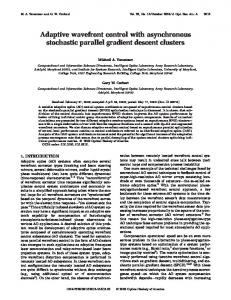
3 by malfunctions of components, for example, errors in programming that lead to infinite cycles. The solution currently recommended in the literature for correcting an infinite cycle is to replace the affected machine by a new machine. The solution proposed in our study is, in many cases, more efficient. Moreover, it is the only practical solution in cases where the affected system is out of reach. The controllers we design are feedback controllers connected to the afflicted machine, as depicted in Figure 1-1. The controller is activated during a cycle. Whenever possible, the controller drives the machine out of the cycle, and leads it to a desirable state. We characterize all cycles from which there is an escape, and present an algorithm for the design of a controller that takes the machine out of any escapable cycle. Σc u

C

v

∑

y

Figure 1-1. Control configuration for the asynchronous sequential machine Σ Here, Σ is the asynchronous machine being controlled, and C is another asynchronous machine that serves as a controller. We denote by Σc the closed loop system represented by Figure 1-1. The controller C eliminates the effects of the cycles of Σ so that the closed loop system Σc matches a prescribed model Σ′ (i.e., Σc = Σ′). The goal is to provide necessary and sufficient conditions for the existence of such a controller C as well as an algorithm for its design. An important property of the controller C is that the closed loop system will function properly whether or not the

4 cycle actually occurs. As a result, the controller C can be used to prevent the effects of cycles before they occur, improving the reliability of the system. It is important to note that during a cycle, the machine moves among unstable states in quick succession, without lingering in any of the cycle states. Consequently, it cannot be arranged for an input change to occur at a specific state of the cycle. Thus, the input changes enforced by the controller occur at random during the cycle, and it is not possible to predetermine the state of the cycle at which the controller acts. As a result, the outcome of the controller action is unpredictable in most cases. This could lead to a critical race condition being generated by the controller, which can then be rectified by known procedures (Murphy (1996); Murphy, Geng and Hammer (2002, 2003); Geng 2003; Geng and Hammer (2003, 2004a, 2004b)). When machine Σ is an input state machine, i.e., the output of Σ is the state of Σ, the controller C is called a state feedback controller. The existence of such a controller C that takes the system out of a cycle depends on certain reachability properties of the system. These reachability properties can be characterized in terms of a numerical matrix called the “skeleton matrix” of the system. The skeleton matrix is calculated from the various transitions of the machine. This skeleton matrix gives a methodology to derive the necessary and sufficient conditions for the existence of a corrective controller C. The function of the controller is two-fold: it eliminates the effects of the cycle on the machine and assigns to the closed loop a specified behavior. The controller C functions by forcing an input character change while the machine is in a cycle; this may induce a critical race. The outcome of this unpredictable behavior is then used by the controller to assign a proper transition, as required to match the operation of the model.

5 In this way, the cycles of the machine are stopped, and the machine exhibits the desired external behavior. The model-matching problem described here is basically a continuation of the work of Hammer (1994, 1995, 1996a, 1996b); Murphy (1996); Murphy, Geng and Hammer (2002, 2003); Geng (2003); and Geng and Hammer (2003, 2004a, 2004b). There are a number of papers that relate to the model-matching problem for synchronous sequential machines (Dibinedetto et al. (1994, 1995a, 1995b, 2001), Barrett and Lafortune (1998)). The studies relating to synchronous machines do not take into consideration the differences between stable and unstable states, fundamental and semi-fundamental mode of operation (Chapter 2), and other issues that are vital to the operation of asynchronous machines. Our study seems to be the first one to explore control theoretic tools to eliminate the effects of infinite cycles on asynchronous machines. Eliminating the effects of infinite cycles is not the only situation in which model matching is beneficial (Dibenedetto et al. (2001)). For example, most large digital system are designed in a modular fashion, with a number of subsystems. An error in the behavior of the machine detected late in the design phase may make it more economical to use a controller instead of redesigning, or rebuilding, the entire machine. In other words, model matching offers a low-cost option to remedy design and construction errors (Fujita (1993)). Moreover, the controller can also be used to improve the reliability and performance of the system, by deploying it before a fault develops in the system. In this way, the controller can guard against potential malfunctions, while being "transparent" before a malfunction occurs. Thus, in machines where high reliability is vital, our study provides a new design option.

6 The early work on automata theory was carried out by Turing (1936). Huffman (1954a, 1954b, 1957) investigated various aspects of the synthesis of asynchronous relay circuits. There is a well established technical literature relating to the subject of design of hazard-free machines (e.g., Liu (1963), Tracey (1966), Kohavi (1970), Maki and Tracey (1971)). This is achieved by appropriate state assignment techniques. Classical methods for hazard free state assignments (Huffman (1954a, 1954b)) are reviewed in most textbooks on digital circuit design (e.g., Kohavi (1970)). More recently, studies on the subject were done by Masuyama and Yoshida (1977), Sen (1985), Datta et al. (1988), Nowick and Dill (1991), Fisher and Wu (1993), Chu (1994), Lavagno et al. (1994), Nowick and Coates (1994), and Lin and Devadas (1995). Evading hazards using a locally generated clock pulse was introduced by Unger (1977), Nowick and Dill (1991), and Moore et al. (2000). A graph theoretic approach for state assignment of asynchronous machines was introduced by Datta, Bandopadhyay and Choudhury (1988). Of course, all the above studies discuss the hazard free design of asynchronous machines, and can be applied only before the machine is constructed; only Murphy (1986); Murphy, Geng and Hammer (2002, 2003); Geng 2003; and Geng and Hammer (2003, 2004a, 2004b) detail methods to overcome hazards in an existing asynchronous machine. Other early works on the synthesis of asynchronous machines were by Mealy (1955) and Moore (1956). These works investigated state and circuit equivalence, and provided methods for synthesizing asynchronous and synchronous sequential machines. Their models of sequential machines are most commonly used today. In the work done by Liu (1963), all internal transitions of a machine go directly from unstable states to terminal states; with no sequencing permitted though stable states. This method of

7 hazard free assignment (called single transition time state variable assignment) uses assignments similar to an equidistant error-correcting code. This kind of assignment, which can be accomplished by mapping the rows of a flow table onto the vertices of a unit n-dimensional cube, is not guaranteed minimal, but it works effectively with incompletely specified flow tables. Tracey (1966) extended this work to techniques that maximize the speed of the machine. A method for sequencing (though unstable states are allowed before a stable state is reached when an input character is applied) was presented by Maki and Tracey (1971), using a technique called the shared row state assignment method. This method generally required fewer state variables than single transition time assignments. Other work on hazard-free state assignment techniques can be found in Hazeltine (1965); McCluskey (1965); Armstrong, Friedman and Menon (1968); Hlavicka (1970); Mago (1971); Chiang and Radhakrishnan (1990); Lavagno, Keutzer and Sangiovanni-Vincentelli (1991); Piguet (1991); Oikonomou (1992); Chu, Mani and Leung (1993); and Fisher and Wu (1993). Some other techniques for avoiding hazards were proposed by Yoeli and Rinon (1964) and Eichelberger (1965). They proposed ternary logic models to analyze certain aspects of the machines. Ternary algebra seems to provide an efficient method for detection and analysis of hazards in sequential circuits. These models were further worked on by Brzozowski and Seger (1987, 1989) and Brzozowski and Yoeli (1987). Another method of avoiding hazards was by generating a clock pulse from other signals in the machine (Bredeson and Hulina (1971), Whitaker and Maki (1992)). Most applications of asynchronous machines assume that the environment of operation is the fundamental mode (Unger (1969)); that is, an input change is applied

8 only after the machine has reached stability. No input change is allowed when the machine transits through unstable states. Our study specifies conditions where fundamental mode is not applicable, leading to what is called semi-fundamental mode of operation (Chapter 2). Recent work in asynchronous sequential machines allows the simultaneous change of several input variables. This mode of operation is referred to as burst-mode (Davis et al. (1993a), Nowick (1993), Yun (1994), and Oliviera et al. (2000)). Deterministic behavior of the machine in this approach needs special restrictions to be imposed on the machine. Plenty of literature is available on the application of control theory to automata and asynchronous machines under discrete event systems. One such example that can be readily quoted is supervisory control (Ramadge and Wonham (1987, 1989)). This is based on formal language theory, and assumes that certain events in the system can be enabled or disabled. The control of the system is achieved by choosing control inputs such that the events are enabled or disabled. Literature on discrete event systems is extensive (Ozveren et al. (1991), Lin (1993), Koutsoukos et al. (2000), Alpan and Jafari (2002), Hubbard and Caines (2002), Park and Lim (2002)). Our study employs finite state machines models, which are more suitable to the investigation of engineering implementations than formal language theory (Dibenedetto et al. (2001)). Asynchronous machines are widely used in industry, as they result in economical digital systems. Some examples of industrial applications are the adaptive routing chip (Davis et al. (1993b)), a cache controller (Nowick et al. (1993)) and the infrared communications chip (Marshall et al. 1994).

9 The organization of this dissertation is as follows. Terminology and background is provided in Chapter 2. A detailed analysis of infinite cycles, detection algorithms, and the existence conditions are detailed in Chapter 3. This chapter also introduced the concepts of generalized state machines, and the use of transition matrices and skeleton matrices in determining the existence of the controller. Chapter 4 gives a detailed solution to the model matching problem for asynchronous sequential machines with cycles, and an algorithm for the construction of the controller. Chapters 3 and 4 contain the necessary and sufficient conditions for the existence of a controller. An example is solved in Chapter 5, detailing the transition and output functions of the controller states, and finally, a conclusion and possible directions of further research are provided in Chapter 6.

CHAPTER 2 TERMINOLOGY AND BACKGROUND 2.1 Asynchronous Machines and States Here, the background and notation is introduced and the basic theory of asynchronous sequential machines is described. An asynchronous machine is activated by a change of its input character; it generates a sequence of characters in response. To explain the mathematical theory, we introduce the notation and terminology involved in describing sequence of characters. An alphabet is a finite non-empty set A; the elements of this set are called characters. A word w over an alphabet A is a finite and ordered (possibly empty) string of characters from A.

Let A be a finite non-empty alphabet, let A* denote the

set of all strings of characters of A, including the empty string, and let A+ be the set of all non-empty strings in A*.

The length |w| of a string w ∈ A* is the number of

characters of w. For two strings w1, w2 ∈ A*, the concatenation is the string w := w1w2, obtained by appending w2 to the end of w1.

A non empty word w1 in A* is a

prefix of the word w2 if w2 = w1w; and w1 is a suffix of the word w2 if w2 = w′w1, where w, w′ ∈ A*. A partial function f : S1→S2 is a function whose domain is a subset of S1 (Eilenberg (1974)). We now introduce the concept of a sequential machine. A sequential machine provides a working mathematical model for a computing device with finite memory. It has the following characteristic properties:

10

11 •

A finite set of inputs can be applied to the machine in a sequential order.

•

There is a finite set of internal configuration that the machine can be in. These configuration are called states, and physically, these states correspond to the setting on the flip flop or the bit combinations in memory devices.

•

The current internal configuration or state and the applied input character determine the next internal configuration or state that the machine achieves. For deterministic systems, the next state is unique.

•

There is a finite set of input characters. There are two broad classes of sequential machines: asynchronous machines and

synchronous machines. An asynchronous sequential machine responds to input changes instantaneously as they occur. On the other hand, a synchronous sequential machine is driven by a clock, and the values of input variables affect the machine only at clock "ticks". The current work concentrates on asynchronous sequential machines. These machine describe the structure of the fastest computing systems. An asynchronous machine is defined by the sextuple Σ := (A,Y,X,x0,f,h), where A, Y, and X are nonempty sets, x0 is the initial state, and f : X×A → X and h : X×A → Y are partial functions. The set A is the set of input values, Y is the set of output values, and X is the set of states. The partial function f is the recursion function and h is the output function. The operation of the machine is described by the recursion xk+1 = f(xk, uk), yk = h(xk, uk), k = 0, 1, 2,…

(2-1)

A valid pair (x,u) ∈ X×A is a point at which the partial functions f and h are defined. We assume that the initial state x0 is provided with Σ. An input sequence is permissible when all pairs (xk, uk), k = 0, 1, 2, ... are valid pairs. The integer k acts as the step counter. An increment in the step counter takes place with every change of

12 the input value or with a state transition. For consistency, we assume that the functions f and h have the same domain. It is clear from the above description that the recursion (2-1) represents a causal system. When the output function h only depends on the state and does not depend on the input, the machine induces a strictly causal system. If the functions f and h are functions rather than partial functions, the machine is said to be complete. A deterministic finite state machine is often referred to as the Mealy machine (Mealy (1955)). If the output function does not depend on the input variable, then the machine is referred to as the Moore machine (Moore (1956)). An asynchronous Mealy machine can be transformed into an equivalent Moore machine, and vice versa. A non-deterministic finite state machine Σ = (A,Y,X,x0,f,h) has the following objects: •

A finite, non-empty set A of permissible input characters, termed as the input alphabet;

•

A finite, non-empty set Y of permissible output characters, termed as the output alphabet;

•

A finite, non-empty set X of states of the machine. Any number of the states can be designates as initial or terminal states;

•

A non-deterministic partial transition function f : β(X)×A → β(X), where β(X) denotes the set of all the subsets of X (i.e., the power set of X);

•

A partial function h : X×A → Y, called the output function; and

•

The initial state of the machine x0 ∈ X. The transition function f can generate sets of states as its values, i.e., f(x,a) = {x1,

…, xk}, rather than just single values; here x1, …, xk ∈ X and a ∈ A. In contrast, the output function h takes only single values, i.e., there can be only one output character

13 associated with each state. The class of deterministic finite state machines is a subclass of non-deterministic finite state machines. The operation of the machine Σ can be described as follows. The machine Σ starts from the initial state x0 and accepts input sequences of the form u := u0 u1 ... , where u0, u1, … ∈ A. In response to this set of applied input characters, it generates a sequence of states x0, x1, x2, … ∈ X and a sequence of output values y0, y1, y2, ... ∈ Y, according to the recursion in Equation 2-1. Finally, the machine Σ is an input/state machine when Y = X and the output is equal to the state at each step, that is, yk = xk, k = 0, 1, 2, …

(2-2)

An input/state machine Σ can be represented by the quadruple (A,X,x0,f), since the output is the state. Using the notion of the transition function f, we can define the partial function f*: X×A+ → X by setting f*(x,u) := f(…f(f(f(x,u0),u1),u2)…,uk) for some state x ∈ X and an input string u = u0u1u2…uk ∈ A+. Thus, f* provides the value of the last state in the path generated by the input string u. For simplicity of notation, we will use f for f*. Some basic terminology important to the study of asynchronous machines is now described. A valid pair (x,u) ∈ X×A of the machine Σ is called a stable combination if f(x,u) = x, i.e., if the state x is a fixed point of the function f. An asynchronous machine will linger at a stable combination until an input change occurs. A pair (x,v) that is not a stable combination is called a transient combination. A potentially stable state x is one for which there is a stable combination. Of course, states that are not potentially stable serve only as transition states; the machine cannot stop or linger in

14 them, and they are not usable in applications. Due to this, it is common practice to ignore states that are not potentially stable; will adhere to this practice and not include such state in our state set. Consider the sequential machine Σ of Equation 2-2. Let x be the state of the machine and u the input value. When a state-input pair (x,u) is not a stable combination, the machine Σ will go through a chain of input/state transitions, starting from (x,u), which may or may not terminate. If the machine reaches a stable combination (x′,u) with the same input value, then the chain of transitions terminates. It must be noted that the input value must remain constant throughout the entire transition; and the transition will end if and only if such a stable combination as (x′,u) exists. In such a case, x′ is called the next stable state of x with input value u. When the next stable state is not uniquely determined, that is, the transition at some point has more than one value, we have a critical race. In case there is no next stable state for x with input value u, we obtain an infinite cycle. Critical races and infinite cycles are the types of hazards that can occur in an asynchronous machine. 2.2 Modes of Operation When the value of an input variable is changed while the asynchronous machine undergoes a chain of transitions, the response of the machine may become unpredictable, since the state of the machine at which the input change occurs in unpredictable. To avoid this potential uncertainty, asynchronous machines are usually operated in fundamental mode, where only one variable of the machine is allowed to change each time. In particular, in fundamental mode operation, a change in the input variable is allowed only while the machine is in a stable combination.

15 One of the main topics of our present discussion relates to the control of an asynchronous machine in an infinite cycle. When a machine is in an infinite cycle, fundamental mode operation becomes impossible, since the machine will not reach a stable combination without a change of the input variable. Nevertheless, we will show later that, when taking the machine out of its infinite cycle, it is not necessary to forego fundamental mode operation for more than one step. When an asynchronous machine operates in fundamental mode in all but a finite number of steps, we say that it operates in semi-fundamental mode. The conditions and procedures for operation in semifundamental mode is described in Chapter 3. Consider a defect-free asynchronous machine Σ = (A,X,x0,Y,f,h) operating in fundamental mode. Let the machine start at the state x0, and be driven by the input string w = v0v1…vm–1. The machine now has transitions through the states x0,…, xm, where xi+1 = f(xi,vi); i = 0,1,2,…,m–1, where the last pair (xm,vm–1) is a stable combination. Fundamental mode operation implies that vi = vi+1 whenever (xi,vi) is not a stable pair, i = 0,…,m–1. The path is defined as the set of pairs P(Σ,x0,w) = {(x0,v0), (x1,v1),…,(xm–1,vm–1), (xm,vm–1)}.

(2-3)

When a cycle occurs, there is no final stable pair, and the path becomes infinite P(Σ,x0,w) = {…,(xi,vj), (xi+1,vj),…,(xi+ ,vj), (xi,vj),…}. As mentioned earlier, the step counter k advances one step during each state transition or input change. Of course, for fundamental mode operation, the input character remains constant during all transition chains.

16 Consider the case where the input value of the machine is kept constant at the character v, while the machine goes through a string of state transitions. At each state transition, the step counter of the system advances by one. This results in the input value being represented as a repetitive string vvv... v, where each repetition corresponds to an advance of the step counter. It is convenient to represent all such repetitions of the input character by a single character, so that, for example, a string of the form w = v0v0v1v1v1v2v2 is represented by w = v0v1v2. Here, it is understood that each input value is repeated as many times as necessary. In the case of an infinite cycle, the input value is repeated indefinitely. Next, let Σ be an asynchronous machine without hazards. Then, the notion of the next stable state leads to the notion of the stable transition function, which plays an important role in our discussion. As the machine Σ has no hazards, every valid pair (x,u) of Σ has a next stable state x′. Define a partial function s : X×A → X by setting s(x,u) := x′ for every valid pair (x,u), where x′ is the next stable state of x with the input character u. The function s is called the stable transition function of the machine Σ. Note that the stable transition function describes the operation of the machine in the fundamental mode, i.e., under the requirement that the input value be changed only after the machine reaches a stable combination. This is a standard restriction in the operation of asynchronous machines, and it guarantees that the machine produces a deterministic response. The stable transition function can be used to describe the operation of an asynchronous machine Σ in the following way. We know that the machine always starts from a stable combination (x0,u-1), at which the machine has been lingering for

17 some time. Suppose now that an input string u := u0u1…uk ∈ A+ is applied to the machine. Then, the machine moves through the a list of states x1, …, xk+1 of next stable states, where xi+1 = s(xi,ui), which implies that (xi+1,ui) is a stable combination for i = 0, 1, …, k. The input list u is permissible if (xi,ui) is a valid combination for i = 0, 1, …, k. Since the machine operates in the fundamental mode, the input character changes from ui to ui+1 only after the stable combination (xi+1,ui) has been reached. This guarantees that the state of the machine is well determined at the time when the input value changes. In general, when a machine does not have infinite cycles, the intermediate transitory states are ignored, as they occur very speedily and are not noticeable by a user. Thus, the operation of an asynchronous machine without infinite cycles, as observed by a user, is best described by the stable transition function s. However, when the machine has infinite cycles, it is not possible to ignore the transitory states involved in the cycle, as the machine lingers among these transitions indefinitely. In Chapter 3, we will introduce a generalized notion of the stable transition function which accommodates infinite cycles by considering them as another form of persistent states. Using the stable transition function s, we define the asynchronous sequential machine Σ|s := (A,X,Y,x0,s,h), which is called the stable state machine induced by Σ. For an input/state machine, the stable state machine is given by the quadruple (A,X,x0,s). To deal with input strings, we can define a partial function s* : X×A+ → X by setting s*(x,u) = s(…s(s(s(x,u0),u1),u2)…,uk), for some state x ∈ X and a permissible input string u = u0u1…uk ∈ A+. The partial function s* provides the last state in the

18 path generated by the input string u. As before, we shall abuse the notation somewhat by using s for s*. In the case where we do not have a Moore machine, we can define the partial function h* : X×A+ → Y in a similar fashion by setting h*(x,u) := h(…s(s(s(x,u0),u1),u2)…,uk) for a state x ∈ X and a permissible input string u = u0u1…uk ∈ A+, as was done for the stable transition function s defined earlier. The partial function h* gives the last output value generated by the input list u. It is necessary in some cases to compare different states of a sequential machine. Two states x and x′ of a machine Σ are distinguishable if the following condition is valid: there is at least one finite input string which yields different output sequences when applied to Σ starting from the initial states x or x′. Two states x and x′ of the machine Σ are equivalent when, for every possible input sequence, the same output sequence is produced regardless of whether the initial state is x or x′. Qualitatively, two states are equivalent if we cannot distinguish them by the input/output behavior of the machine. If two states are equivalent, then so are all corresponding states included in any paths started from x and x′. If a machine Σ contains two equivalent distinct states, then one of the states is redundant, and it can be omitted from the mathematical model of the machine. A machine Σ is minimal or reduced if it has no distinct states that are equivalent to each other. Consider two machines Σ = (A,Y,X,f,h) and Σ′ = (A′,Y′,X′,f′,h′). Let x be a state of Σ and let x′ be a state of Σ′. The states x and x′ are equivalent if both have the same permissible input sequences, and if, for every permissible input sequence, the output sequence generated by Σ from the initial state x is the same as the output

19 sequence generated by Σ′ from the initial state x′. The two machines Σ and Σ′ are equivalent whenever there exists an equivalent state in Σ for every state in Σ′, and similarly, an equivalent state in Σ for every state in Σ′. A number of texts dwell on the various aspects of the theory of sequential machines and automata, including McCluskey (1965); Arbib (1969); Kalman, Falb and Arbib (1969); Kohavi (1970); Eilenberg (1974); and Evans (1988).

CHAPTER 3 INFINITE CYCLES 3.1 Introduction An infinite cycle is caused when there is no next stable state for a valid pair (x,u) of a finite state asynchronous machine Σ = (A,X,x0,Y,f,h). In such case, the machine will keep moving indefinitely from one transient combination to another. Only a finite number of states can be involved in these transitions, since Σ is a finite state machine. An infinite cycle can then be characterized by listing these states and the corresponding input which causes the infinite cycle. Specifically, let the state set of Σ be X = {x1, x2, ..., xn}. Consider a infinite cycle ρ of Σ that involves p states, say the states xk1, xk2, ..., xk ∈ X, and let a ∈ A be the input character causing the infinite cycle. The infinite cycle then functions according to the recursion xkj+1 = f(xkj, a), j = 1, ..., –1, and xk1 = f(xk , a).

(3-1)

As a shorthand notation, we will use ρ = {a;xk1, xk2, ..., xk }, where a is the input character of the infinite cycle, and xk1, xk2, ..., xk are its states. A state-input pair (xkj ,a), for some j = 1, …,

is then said to be a pair of the cycle ρ. The length

of the

infinite cycle ρ is defined as the number of distinct states it contains. It follows that a cycle of length

has

distinct input-state pairs. A brief examination of Equation 3-1

leads to the following conclusion: Let (x,a) be any pair of the infinite cycle ρ. Then, x′

20

21 is a state of ρ if and only if there is an integer j such that x′ = fj(x,a). Then, the recursion can be followed for the entire length of the cycle. It is convenient to denote by {fj(x,a)}j=0 the set of all distinct states included in the set {x, f(x,a), f2(x,a), ...}. This leads us to the following lemma. Lemma 3-1 Let (x,a) be any pair of the infinite cycle ρ. Then, the state set of ρ is {fj(x,a)}j=0. ♦ Lemma 3-1 gives a way of finding the states of a cycle. A machine can have several infinite cycles, and we demonstrate below an algorithm that finds all infinite cycles of a given machine. It is relevant to see that an infinite cycle of length 1 is nothing but a stable combination. To distinguish between infinite cycles and stable combinations, the length of an infinite cycle must at least be 2. According to the next statement, infinite cycles associated with the same input character must have disjoint state sets. Lemma 3-2 A valid input/state pair (x,a) of an asynchronous machine Σ can be a member of at most one infinite cycle. Proof 3-2. Let ρ1 and ρ2 be two infinite cycles of the machine Σ associated with the same input character a. If ρ1 and ρ2 contain the same pair (x,a), then, using Lemma 3-1, we conclude that ρ1 and ρ2 have the same state set. In other words, ρ1 = ρ2, and our proof concludes. ♦ The above Lemma 3-1 gives us an insight into the structure of the cycle. Since no state can be a member of more than one cycle, we can say that a pair of a cycle is unique to that cycle. We can now find a bound on the maximal number of infinite cycles a

22 machine can have. Indeed, consider the set of all infinite cycles involving the input character a. In view of Lemma 3-2, all such infinite cycles have disjoint state sets. But then, the fact that a infinite cycle must contain at least 2 states, implies that there cannot be more than n/2 such infinite cycles, where n is the number of states of the machine. Finally, recalling that the machine has m input characters, we obtain the following. (Denote by [a]– the largest integer not exceeding a.) Proposition 3-3 Let Σ be a sequential machine with n states and an alphabet A consisting of m characters. Then, Σ cannot have more than m[n/2]– infinite cycles. ♦ For the sake of brevity, “infinite cycles” will be referred to as just “cycles” in the rest of the document. 3.2 Detection of Cycles In this section, a procedure to detect the cycles associated with a machine will be outlined. Consider an asynchronous machine Σ = (A,X,x0,Y,f,h) with n states and an alphabet A of m input characters. Next all the cycles of the machine Σ will be determined. To this end, an n×n matrix M(f) is recursively constructed as follows. The (i,j) entry of M(f) is the set of all characters u ∈ A for which xi = f(xj,u). If there is no input character u ∈ A for which xi = f(xj,u), then the (i,j) entry of M is denoted Γ, where Γ is a character not included in the alphabet set A. Thus, the matrix becomes

⎧⎪ u ∈ A : x i = f(x j ,u), Mi,j(f) := ⎨ ⎪⎩Γ otherwise,

(3-2)

i, j = 1, ..., n. Multiple entries in a cell are separated using a comma. We refer to M(f) as the one-step transition matrix of the machine Σ.

23 We now define two matrix operations for one-step transition matrices. First, the sum of two n×n one-step transition matrices A and B is defined element wise by

(A ∪ B)ij := Aij ∪ Bij, i, j = 1, ..., n.

(3-3)

The sum operation is reminiscent of the numerical addition of matrices. The following operations on members of the set A ∪ Γ is now defined. ΓΓ := Γ u1Γ := Γ Γu1 := Γ u1u1 := u1 u1u2 := Γ Γ ∪ Γ := Γ

(3-4)

u1 ∪ Γ := u1 u1 ∪ u1 := Γ u1 ∪ u2 := Γ Also, for any two sets, the operation of multiplication is defined by {a1, a2, ..., aq}.{b1, b2, ..., br} = {aibj}i=1, ...,q, j=1, ...,r This is similar to the classical definition of the scalar product of two vectors. Using these operations of multiplication, the definition of matrix combination is defined as follows. (AB)ij := ∪k=1, ..., nAikBkj for all i, j = 1, ..., n.

(3-5)

Consider two functions g, h : X×A → X. The composition of g and h is defined by gh(x,u) := g(h(x,u),u). The composition of function is closely related to the combination of the corresponding one-step transition matrices, as indicated by the following. The next statement shows that the multiplication of two one-step transition

24 matrices on two recursion functions is the transition matrix on the composition of the two functions. Lemma 3-4 Let g, h : X×A → X be two recursion functions with one step

transition matrices M(g) and M(h), respectively. Then, M(g)M(h) = M(gh). Proof 3-4. Using Definition 3-4, we have

M(g)M(h) = ∪k=1..n Mi,k(g)Mk,j(h).

(3-6)

Now, each entry of M(g)M(h) is either a character of A or Γ; the definition of matrix composition implies that the following two statements are equivalent: (i) The (i,j) element of M(g)M(h) is u. (ii) There is a k ∈ {1, ..., n} for which Mi,k(g) = u and Mk,j(h) = u. When (ii) holds, we have xi = g(xk,u) and xk = h(xj,u), so that xi = g(h(xj,u),u) = gh(xj,u). Then, the (i,j) entry of M(gh) is u. Conversely, if the (i,j) entry of M(gh) is u, then xi = gh(xj,u), so that xi = g(h(xj,u),u). Now, the value h(xj,u) is, by definition, an element of X, say the element xk, k ∈ {1, ..., n}. Then, xk = h(xj,u) and xi = g(xk,u), which implies that (ii) is valid for this k. Thus, we have shown that (ii) is equivalent to (iii) Mi,j(gh) = u. Using the fact that (ii) is equivalent to (i), the Lemma follows. ♦ Thus, the product of two transition matrices with two different transition functions is the transition matrix of the composition of the two functions in the order of multiplication. Consider now the a machine Σ with recursion function f. Let M(f) be

25 its one-step transition matrix. Then, by Lemma 3-4, M(f)M(f) = M(f2), M(f2)M(f) = M(f3), and so on. This leads to the following corollary. Corollary 3-5 Let Σ = (A,X,x0,Y,f,h) be an asynchronous machine. Then, for

every integer p > 0, the one-step transition matrix satisfies Mp(f) = M(fp). ♦ Consider a machine Σ = (A,X,x0,Y,f,h). As mentioned earlier, a stable combination (x,u) of Σ can be considered as a cycle of length 1. This observation helps simplify the following statement, which forms an important tool in our process of finding all cycles of the machine Σ. Lemma 3-6 Let Σ be an asynchronous machine with the recursion function f and

the state set X = {x1, ..., xn}. Let xi ∈ X be a state and let u be an input character of Σ. Then, the following three statements are equivalent. (i) There is an integer τ ≥ 1 such that xi = fτ(xi,u) (ii) u appears on the (i,i) diagonal entry of the matrix Mτ(f). (iii) (xi,u) is a pair of a cycle whose length λ is an integer divisor of τ. Proof 3-6. First, we show that (i) implies (ii). Assume that (i) is valid, so that xi =

fτ(xi,u) for some integer τ ≥ 1. Then, by Equation 3-2, the character u appears on the diagonal entry (i,i) of the matrix M(fτ). By Corollary 3-5, M(fτ) = Mτ(f); this implies that u appears on the diagonal entry (i,i) of the transition matrix Mτ(f). Next, we show that (ii) implies (iii). Let λ ≥ 1 be the smallest integer satisfying xi = fλ(xi,u). Then, λ ≤ τ. Now, if λ = 1, then (xi,u) is a stable combination of Σ, and hence forms a cycle of length 1. Otherwise, (xi,u) is a pair of the cycle {xi, f(xi,u), ..., fλ–1(xi,u); u} of length λ.

26 Now, using the integer division algorithm, we can write τ = qλ + ρ, where q and ρ are integers and 0 ≤ ρ < λ. If ρ > 0, then, using the equality xi = fλ(xi,u), we can write xi = fτ(xi,u) = fρ(fqλ(xi,u),u) = fρ(xi,u), so that xi = fρ(xi,u). The latter contradicts the fact that λ was the smallest integer satisfying xi = fλ(xi,u), since 0 < ρ < λ. Thus, we must have ρ = 0, and λ must be an integer divisor of τ. Finally, we show that (iii) implies (i). Assume that (iii) is valid, i.e., that (xi,u) is a pair of a cycle whose length λ is a divisor of τ. Then, there is an integer q such that τ = qλ. But then, fτ(xi,u) = fqλ(xi,u) = xi, and (i) is valid. This concludes the proof. ♦ Thus, by taking the powers of the one-step transition matrix M(f) and observing the diagonal matrix at each step, the states of the machine involved in cycles can be isolated. The next lemma indicates a method of identifying the elements of each cycle. Lemma 3-7 Let Σ be an asynchronous machine with state set X = {x1, ..., xn}

and recursion function f. Assume that Σ has a cycle of length λ > 1 that includes the pair (xj0,u). Then, the other states xj1, ..., xjλ–1 of the cycle can be found from the matrix M(f) in the following way: for every integer i = 0, ..., λ–2, the index ji+1 is given by the position of the entry u in the column ji of the matrix M(f). Proof 3-7. Consider a cycle of length λ > 1. Let {xj0, xj1, ..., xjλ–1} be the states

involved in the cycle, and let u be the input character. We know f(xj0,u) = xj1. This implies that the input character u appears exactly in the position (j0, j1) of the matrix M(f). Thus, the value of j1 is given by the position of the character u in the row j0. Continuing recursively, assume that, for some 0 ≤ k < λ, the indices j0, j1, ..., jk of the states xj0, xj1, ..., xjk of the cycle have been found. Then, since xjk+1 = f(xjk,u), the

27 character u will appear exactly in position jk+1 of the row jk of the matrix M(f). This concludes our proof. ♦ Thus, the knowledge of the states involved in cycles of a particular length can be used to find the cycles specifically by applying Lemma 3-7. An algorithm that finds all the cycles of an asynchronous machine Σ whose recursion function is f will now be outlined. Let #A denote the number of elements in the set A. Algorithm 3-8 Let Σ = (A,X,x0,Y,f,h) be an asynchronous machine, and let M(f)

be its transition matrix. Step 1: All entries on the main diagonal of M(f) represent stable combinations (i.e., cycles of length 1). For each input character u ∈ A, let ∆1(u) be the set of all states for which u is included in a diagonal entry of the matrix M(f); set ϑ1(u) := ∆1(u). Step 2: For i ≥ 2, let ∆i(u) be the set of all states for which u is included in a diagonal entry of the matrix Mi(f). Define the difference set ϑi(u) := ∆i(u) \ ∪1 ≤ j ≤ i–1 ∆j(u).

(3-7)

Stop the algorithm for the character u when i+1 > n – Σij=1 #ϑj(u). ♦ The significance of Algorithm 3-8 is pointed out by the following statement. Proposition 3-9 Let i ≥ 1 be an integer. Then, in the notation of Algorithm 3-8,

the following are true. (i) The set ϑi(u) consists of all states of the machine Σ that are members of cycles of length i with the input character u. (ii) The machine Σ has exactly #ϑi(u)/i cycles of length i.

28 Suppose there are 2λ states in ϑλ(u). This means there are 2 cycles of length λ in the machine. Pick one state from ϑλ(u); use Lemma 3-7 to find the other λ–1 members of that cycle. Now, pick another state from the λ remaining states in ϑλ(u), and using Lemma 3-7, the second cycle can be determined. This procedure is extended to any number of cycles of a certain length. Proof 3-9. Let X = {x1, ..., xn} be the state set of Σ, and let u ∈ A be a character

of the input set. By Lemma 3-6, the following two statements are equivalent: (a) The matrix Mi(f) has an entry including u on its main diagonal, in a column that corresponds to the state xr of Σ. (b) The state xr is a member of a cycle whose length is i or an integer divisor of i. The case i = 1 is simple, since the elements on the main diagonal of M(f) represent the stable combinations of the system, and whence the cycles of length 1. For i > 1, assume that the algorithm has not stopped before i, i.e., that i ≤ n – Σij=1 #ϑj(u). Then, a slight reflection shows that the construction Equation 3-7 of ϑi(u) removes all states that are included in cycles of length less than i. Combining this with the equivalence of (a) and (b), it follows that xr ∈ ϑi(u) if and only if xr is a member of a cycle of length i. Finally, consider the case where i+1 > n – Σij=1 #ϑj(u), and υ(u) be the number of states of Σ that are members of cycles of length λ ≤ i with the character u. From the definition of ϑj(u), it follows that υ(u) = Σij=1 #ϑj(u). Thus, when i + 1 > n – υ(u), there are not enough states left to form a cycle of length i + 1 with the character u; whence

29 the machine Σ has no cycles of length greater than i with the character u. This completes the proof of part (i) of the Proposition. Regarding part (ii) of the Proposition, note that the set ϑi(u) consists of all states that form cycles of length i with the input character u. By Lemma 3-2, no two cycles can have common states. Consequently, the number of elements of ϑi(u) is a multiple of i, and the number of cycles in ϑi(u) is given by #ϑi(u)/i. This concludes our proof. ♦ 3.3 Stable State Representations for Machines with Cycles

In this section, a form of representation of only the next stable states and the extension of the definitions to the case of a machine with cycles will be explained. For an asynchronous machine Σ = (A,X,Y,x0,f,h) without cycles, a valid pair (x,u) always has a next stable state x′. Consequently, for such a machine, one can define a partial function s : X×A → X by setting s(x,u) = x′ for every valid pair (x,u). The function s is then called the stable recursion function of the machine Σ. When s is used as a recursion function, it induces the stable-state machine Σ|s = (A,X,Y,x0,s,h). The stable state machine describes only persistent states of the machine, and ignores unstable transitions. This function describes the behavior of Σ as experienced by a user, i.e., the transition of the machine to its next stable state is described. A reformulation of the finite state machine with cycles will now be explained, so that an equivalent stable state machine can be described from this reformulated machine. As mentioned earlier in Chapter 2, asynchronous machines are normally operated in fundamental mode. In specific terms, fundamental mode operation is as follows. Let Σ be an asynchronous machine without cycles, resting in a stable combination (x,u0).

30 Consider a string of input values u = u1…uk ∈ A+ applied to the machine. When the input of Σ switches to u1, the machine may engage in a string of transitions culminating in the next stable state s(x,u1). In fundamental mode operation, the input character u1 is kept fixed until the machine has reached its next stable state, to guaranty deterministic behavior. Then, once the machine reaches the stable combination (s(x,u1),u1), the input character is switched to u2, and the machine eventually settles on its next stable state s(s(x,u1),u2). This process continues until we reach the final input value uk. The last stable state reached in this process is given by x" := s(…(s(s(s(x,u0),u1),u2)…,uk). To simplify our notation, we shall write in brief x" := s(x,u). As mentioned earlier, the stable state machine describes persistent states of an asynchronous machine. For machines with cycles, a cycle describes a persistent state of the machine (i.e., the "state" of being in a cycle). Hence, when cycles are present, they must be represented in the stable state machine. Our next objective is to generalize the definition of the stable state machine, so it gives due representation to cycles, whenever they are present. Consider an asynchronous machine Σ = (A,Y,X,x0,f,h) having t > 0 cycles ρ1, ..., ρt. To define a stable state machine Σ|s that represents the persistent behavior of Σ, we first augment the state set X of Σ by t new elements xn+1, ..., xn+t to obtain the augmented state set Xρ := X ∪ {xn+1, ..., xn+t}.

(3-8)

Each one of the new states, called the cycle states, corresponds to one of the cycles of Σ, i.e., xn+i corresponds to the cycle ρi, i = 1, ..., t.

31 Define the function s′ : X×A → Xρ by setting ⎧⎪s(x,u) if x ∈ X and (x,u) is a stable combination, s1(x,u) = ⎨ n+1 if (x,u) ∈ ρi . ⎪⎩ x

(3-9)

For a cycle ρ = {xk1, xk2, ..., xkp;a}, ki ∈ [1,…,n], denote s1[ρ,u] := {s1(xk1,u), s1(xk2,u), ..., s1(xkp,u)}.

(3-10)

Now, the function s2 : Xρ×A → Xρ is defined by setting ⎧⎪s1 (x,u) if x ∈ X, s2(x,u) := ⎨ 1 n+i ⎪⎩s [ρi ,u] if x = x .

(3-11)

The generalized stable state machine Σ|s of Σ is then the input/state machine defined by quintuple (A,Xρ,x0,s2). For the sake of notational convenience, we will omit the primes from s2 in the future, and write Σ|s = (A,Xρ,x0,s). The function s is called the generalized stable recursion function of Σ. A cycle ρ associated with a cycle state x is said to be stoppable if there exists an input character u ∈ A such that at least one of the outcomes of s(x,u) ∈ X. In the present work, we assume that all the cycles are stoppable. It is necessary to make this assumption; if not, there will be no controller that can stop the cycle. Note that when there are no cycles, the generalized stable recursion function of Σ is identical to the stable recursion function of Σ. Let Σc|s be the generalized stable state machine induced by the closed loop system Σc shown in Figure 1-1. The present work concentrates on finding the solution to the next statement; consequently, this statement is the main topic of our discussion.

32 The Model Matching Problem 3-10 Let Σ be a machine and let Σ′ be a stable

state machine with the same input and output alphabets as Σ. Find necessary and sufficient conditions for the existence of a controller C such that the generalized stable state machine Σc|s = Σ′. When C exists, provide a method for its design. ♦ The controller C of Problem 3-10 assigns to closed loop system the stable state behavior of the specified machine Σ′. Of particular interest to us here is the case where the machine Σ has infinite cycles. In such case, the controller C of 3-10 eliminates the effect of infinite cycles on the closed loop system. The model matching problem for asynchronous machines with critical races, but not infinite cycles, was discussed in Murphy 1996, Murphy, Geng and Hammer 2002, 2003, Geng 2003- In the following section, a solution for the model matching problem for the case where the controlled system Σ has infinite cycles is derived, and in Chapter 5 the design of an appropriate controller is demonstrated by means of an example. 3.4 Stable Reachability

The extension of the stable state machine to machines with cycles will now be described. This requires a reformulation of the machine. Consider an asynchronous machine Σ represented by the sextuple (A,Y,X,x0,f,h), and assume that Σ has t > 0 cycles ρ1, ..., ρt. Let Σ|s = (A,Xρ,x0,s), where Xρ = X ∪ {xn+1, ..., xn+t}, and xn+i is the generalized state corresponding to the cycle ρi. We aim to define the notion of stable reachability for the machine Σ so as to characterize the "stable" states Σ can reach from a given initial condition, in response to various input strings. To this end, we need to define several notions. A generalized stable combination of the machine Σ is either a

33 stable combination of Σ or a pair of the form (xn+i,u), where u is the input character of the cycle ρi. A state of Σ|s is potentially stable if it is part of a generalized stable combination of Σ. When applying a control input to a machine that is in an cycle, it is not possible to operate in the fundamental mode. The input character must be changed while the cycle is in progress in order to attempt to interrupt the cycle. In other words, the input character is changed while the machine is not in a stable combination. Of course, if this change in input leads the machine to a stable combination, then fundamental mode operation can be resumed from there on. We arrive at the following notion, which describes the mode of operation that is closest to fundamental mode operation. Definition 3-11 A machine Σ is said to operate in semi-fundamental mode if the

machine operates in fundamental mode when it is not in an cycle. ♦ Recall that the states of the generalize stable-state machine Σ|s are either potentially stable states of Σ or cycle state that represent cycles. Thus, semifundamental mode operation of Σ becomes fundamental mode operation of Σ|s. Definition 3-12 Let Σ be an asynchronous machine with generalized state set Xρ

and generalized stable recursion function s. A state x′ ∈ Xρ is stably reachable from a state x ∈ Xρ if there is a input string u = u0u1…uk of Σ for which x′ = s(x,u). ♦ The following assumption is essential in determining the controller operation. If an input character forms a valid combination with one outcome of a critical race, then it forms a valid combination with all other outcomes of the same race. This assumption can always be satisfied by extending the definition of the recursion function of the machine.

34 It is necessary to assume this statement because we need the controller to be operational will all outcomes of the critical race that follows the cycle. 3.5 Matrix of Stable Transitions and the Skeleton Matrix

Consider an asynchronous machine Σ = (A,Y,X,x0,f,h) with the state set { x1, ..., xn}, and assume that Σ has t > 0 cycles ρ1, ..., ρt. Let Σ|s = (A,Xρ,x0,s), where Xρ = X ∪ {xn+1, ..., xn+t} and xn+i is the generalized state corresponding to the cycle ρi. Let sx(xj,xi) be the set of all characters u ∈ A such that xi ∈ s(xj,u). The matrix of one-step generalized stable transitions gives all the possible stable one-step transitions of the

machine Σ|s; it is an (n+t)×(n+t) matrix R(Σ|s), whose (i,j) entry is given by ⎪⎧s x (x j ,x i ) if s x (x j ,x i ) ≠ ∅, Rij(Σ|s) = ⎨ ⎪⎩ N otherwise,

(3-12)

i, j = 1, ..., n+t. Recall that, if xj is a generalized state, then a critical race may occur when an input character u is applied at xj. This race is represented in the matrix R(Σ|s) by the appearance of the character u in more than one row of column j. Note that Equation 3-12 is similar to Equation 3-2, except for the fact that R(Σ|s) has some augmented states instead of cycles. We turn now to a description of some operations on the matrix R(Σ|s). Let A* be the set of all words over the alphabet A. The operation of unison ∪/ is defined over the set A* ∪ N as follows. Let w1, w2 be either subsets of the set A* or the character N; then, set

35 ⎧ w1 ∪ w 2 if w1 ⊂ A* and w 2 ⊂ A*, ⎪ w if w ⊂ A* and w = N, ⎪ 1 2 w1 ∪/ w2 := ⎨ 1 ⎪ w 2 if w1 = N and w 2 ⊂ A*, ⎪⎩ N if w1 = w 2 = N.

(3-13)

Extending this definition to matrices, the unison C := A ∪/ B of two n×n matrices A and B is defined by Cij := Aij ∪/ Bij, i, j = 1, ..., n, i.e., an element-wise operation as defined in Equation 3-13As usual, the concatenation of two words w1, w2 ∈ A* is given by w1w2, i.e., w1 followed by w2. For elements w1, w2 are elements of A* or the character N, the concatenation is defined as follows. ⎧ w w if w1 , w 2 ∈ A*, conc(w1,w2) := ⎨ 1 2 ⎩ N if w1 = N or w 2 = N.

(3-14)

More generally, let W = {w1, w2, …, wq} and V = {v1, v2, …, vr} be two subsets, whose elements are either words of A* or the character N. Define conc(W,V):= ∪/ i=1,...,q conc(wi,vj).

(3-15)

j=1,...,r

Note that the concatenation is either a subset of A*, or it is the character N. The concatenation is non-commutative, and N takes the place of a "zero". Let C and D to be two n×n matrices whose entries are subsets of A* or the character N. Let Cij and Dij be the (i,j) entries of the corresponding matrices. Then, the product Z := CD is an n×n matrix, whose (i,j) entry Zij is given by n

Zij := ∪/ k=1conc(Cik,Dkj), i,j = 1, …, n.

(3-16)

36 Using this notation, we can define powers of the one-step transition matrix recursively, by setting Rµ(Σ|s) := Rµ–1(Σ|s)R(Σ|s), µ = 2, 3, …

(3-17)

The matrix Rµ(Σ|s) has the following physical significance. The (i,j) element of Rµ(Σ|s) is the set of all input strings that take xj to xi in exactly µ steps. Thus, Rµ(Σ|s) is called the matrix of µ-step stable transitions. This follows from Corollary 3-5, which states that the powers of the one-step transition matrix is equal to the transition matrix of the powers of the recursion function, i.e., the steps of the transition matrix. Define the matrix R(µ)(Σ|s) := ∪/ k=1...µ Rk(Σ|s), v=2,3,...,(n+t–1).

(3-18)

By construction, the (i,j) entry of R(µ)(Σ|s) consists of all strings that can take the machine Σ|s from the state xj to the state xi in µ or fewer steps. The following statement is important to our discussion; the proof is similar to that of Murphy, Geng and Hammer, 2003, Lemma 3-9. Lemma 3-13 The following two statements are equivalent:

(i) There is an input string that can take the machine Σ|s from the state xj to the state xi. (n+t–1)

(ii) The i,j entry Rij

(Σ|s) ≠ N. ♦

Now, R(n+t–1)(Σ|s) contains not only the stable transitions, but also the critical races that are cause when an input character is applied to a cycle state. To satisfy the model matching problem, we need a matrix for which the same input string does not lead to

37 multiple outcomes. This is achieved by modifying the above matrix. This modified matrix is at the center of our discussion. Definition 3-14 Let Σ be an asynchronous machine. The matrix of stable transitions T(Σ|s) is constructed by performing the following operation on each column

of the matrix R(n+t–1)(Σ|s): remove all occurrences of strings that appear in more than one entry of the column; if empty entries result, replace them by the character N. ♦ To understand the significance of the matrix T(Σ|s), it is instructive to compare it to the matrix R(n+t–1)(Σ|s). A string u in the (i,j) entry of the matrix R(n+t–1)(Σ|s) indicates, of course, that u takes Σ|s from xj to xi. However, if the string u appears in another entry in column j of R(n+t–1)(Σ|s), say in entry k, then the same string may also take Σ|s from xj to xk; this indicates a critical race. The construction of the matrix T(Σ|s) removes then all transitions that involve critical races. As a result, an input string u that is included in the (i,j) entry of T(Σ|s) takes the machine Σ|s from the state xj to the state xi, and to no other state. Definition 3-15 Let Σ be an asynchronous machine with the generalized state set

{x1, ... xn+t}. A generalized stable transition from a generalized state xj to a generalized state xi is a uniform transition when one of the following is true: (i) xi can be reached from xj without passing through a critical race, or (ii) there is a succession of critical races through which xi can be reached from xj for all possible race outcomes. ♦ Note that in case (ii) of Definition 3-15, the input string applied to the machine may depend on the outcomes of the critical races encountered by the machine along its way from the state xj to the state xi. Specifically, let x(k,p) be outcome k of race p along

38 the way from xj to xi. The input string applied to the machine will then be a function of the outcomes u(x(k1,1,1), ..., x(k1,p1,p1)) . The set ∪a = 1,…,ru(x(kr,1,1), ..., x(kr,pr,pr)) is (i,j) transition set, where r is the number of possible input strings taking into account all

the critical races encountered in the path from xj to xi. This means that pr races are encountered in the path followed by the rth string, and x(kr,pr,pr) is the outcome kr,pr of the race pr. Further, By construction, the elements of T(Σ|s) will contain sets of strings that satisfy the following proposition. Proposition 3-16 The (i,j) entry of T(Σ|s) is different from N if and only if there

is a uniform transition from xj to xi. Furthermore, if the (i,j) entry of T(Σ|s) is not N, then it includes an (i,j) transition set. ♦ Thus, depending on the sequence of critical races that occur, the entries of T(Σ|s) gives a set of strings that can be used for the control process. The skeleton matrix is now defined as follows matrix: Definition 3-17 Let T(Σ|s) be the matrix of stable transitions of the generalized

stable state machine Σ|s. The skeleton matrix K(Σ) of Σ is a matrix of zeros and ones, whose (i,j) entry is given by

⎧⎪1 if Tij (Σ|s ) ≠ N, Kij(Σ) = ⎨ ⎪⎩0 otherwise

(3-19)

i = 1,…,n, j = 1,…,n+t. ♦ The skeleton matrix K(Σ) has a simple interpretation. In view of Lemma 3-13, the following is true

39 Proposition 3-18 Let K(Σ) be the skeleton matrix of a given machine Σ. Then,

the (i,j) entry of K(Σ) is 1 if and only if there exists a string that takes the machine Σ|s from the generalized state xj to the state xi and to no other state. ♦ The skeleton matrix plays a critical role in our discussion, reminiscent of the role it played in Murphy, Geng and Hammer 2002, 20033.6 Corrective Controllers

The basic considerations in the construction of a corrective controller and its limitations for asynchronous input/state machines will now be outlined. Let Σ be an asynchronous machine, being controlled in the configuration Figure 1-1 with the controller C. Recall that Σc denotes the closed loop machine of Figure 1-1; let Σc|s be the stable state machine induced by Σc. Now, let Σ′ = (A,X,x0,s′) be a stable state input/state machine, with the same input set and the same state set as the machine Σ. Referring to the configuration Figure 1-1 and the Model Matching Problem 3-10, we are investigating the existence of a controller C for which Σc|s = Σ′. Consider the input/state machine Σ = (A,X,X,f,h) and the controller C = (A×X,A,Ξ,φ,η). Let the generalized stable state machine associated with Σ be Σ|s. As shown below, the controller C will operate in the semi-fundamental mode: when the controlled machine Σ moves toward a stable combination, the controller C will operate in fundamental mode - it will keep its output value constant until Σ has reached its next stable combination; however, if Σ moves into an infinite cycle, the controller has no choice but to change its output value while Σ is cycling - otherwise, Σ will remain in the cycle forever. In this case, the controller operates in the semi-fundamental mode.

40 Recalling that Σ has the state set X and that C has the state set Ξ, it follows that the composite machine Σc of Figure 1-1 has the state set X×Ξ. We can then represent Σc by the quintuple (A,X,X×Ξ,fc,hc), where fc is the recursion function of Σc and hc is its output function. Being an input/state system, the machine Σ has the output function h(x,u) = x. As the output of Σc is the same as the output of Σ, it follows that hc(x,ξ,v) = x. Formally, let πx : X×Ξ→X : πx(x,ξ)

x be the standard projection.

Then, we have hc = πx. Now, let γ be the recursion function of Σc|s. We know that the output of Σc|s is the state of Σ. So, if Σc|s = Σ′, then, for every valid pair (x,v) of Σ′, there is a state ξ ∈ Ξ for which (x,ξ,v) is a valid pair of Σc|s. This leads to the conclusion hcγ(x,ξ,v) = s′(x,v),

(3-20)

and, using the equality hc = πx, we obtain πxγ(x,ξ,v) = s′(x,v). Note that, if s′ is not constant over one of the cycles, then the response of the closed loop machine will depend on the state of the cycle at which the input character is applied, creating a critical race. In other words, in order for the response of the closed loop system to be deterministic, the stable recursion function of the model must be constant over each cycle of the controlled machine Σ. To state this fact formally, consider a cycle ρ = {xk1, xk2, ..., xkp;a}, ki ∈ [1,…,n], of the machine Σ. Let s′{ρ} := {s′(xk1,a), ..., s′(xkp,a)}, i.e., the set of values of s′ over the cycle. We say that s′ is constant over the cycle ρ if all members of the set s′{ρ} are identical.

41 Proposition 3-19 Let Σ and Σ′ be two machines, where Σ′ is a stable state

machine. Assume that there is a controller C such that Σc|s = Σ′. If the closed loop machine Σc|s has a race free response, then the recursion function s′ of the model Σ′ is constant over every cycle of Σ. ♦ We are now ready to state one of the main results of our discussion. The following theorem deals with the fundamental conditions for the existence of a model matching controller (compare to Murphy, Geng and Hammer 2002, 2003, Theorem 4.3). Before stating the theorem, we need some notation. For a cycle state z ∈ Xρ, let ρ(z) = {a; xk1, xk2, ..., xkp}, ki ∈ [1,…,n], be the corresponding cycle, and let πxρ(z) := {xk1, xk2, ..., xkp } be the states of the cycle. Define ⎧z if z is a regular state, ϕ(z) = ⎨ ⎩ π x ρ(z) if z is a cycle state.

(3-21)

Note that ϕ(z) is always a set of regular states, not cycle states. Theorem 3-20 (Existence of Controller) Let Σ|s = (A,Xρ,x0,s) be the generalized

stable state machine induced by an input/state machine Σ = (A,X,x0,f). Let z1, ..., zk be generalized states of Σ|s and let U1, ..., Uk be sets of input characters such that z1×U1, z2×U2, …, zk×Uk are distinct sets of valid pairs of Σ|s. For each i = 1, ..., k, let z′i be a state of Σ that is stably reachable from the generalized state zi. Then, there exists a controller C for which Σc|s is equivalent to a stable state machine Σ′ = (A,X,x0,s′), whose recursion function s′ satisfies (i) s′[ϕ(zi),Ui] = z′i for all i = 1,…,k, and (ii) s′(x,t) = s(x,t) for all (x,t) ∈ X×A / ∪i=1,…,k zi×Ui.

42 Moreover, the closed loop system Σc is well posed, and it operates in the semifundamental mode. Proof 3-20. By Proposition 3-19, the recursion function of the model is constant

over all cycles of the machine Σ. Thus, since z′i is stably reachable from the generalized state zi, there exists a string wi ∈ A+ such that s(zi,wi) = z′i, where s is the 0 1

m(i)–1

stable recursion function of Σ. Let m(i) be the length of wi; write wi = vi vi …vi 1

m(i)–1

where v0i, vi , …, vi

,

are individual characters of the input alphabet A and i = 1, …,

k. With this input string wi, the recursion function s generates a string of generalized states, which we denote by 0

xi,1 := s(zi,vi ), 1

xi,2 := s(xi,1,vi ), …, m(i)–2

xi,m(i)–1 := s(xi,m(i)–2,vi

),

m(i)–1

z′i := s(xi,m(i)–1,vi

), i = 1, …, k.

(3-22)

Let U(zi) ⊂ A be the set of all input characters that form stable combinations with the generalized state zi, i = 1, …, k. Define the following sets: S := ∪i=1, …, k zi×U(zi), V := ∪i=1, …, k zi×Ui,

(3-23)

where Ui are the input character sets given in the statement of the Theorem. Then, a controller C = (A×X,A,Ξ,φ,η) that satisfies the requirements of Theorem 3-20 can be constructed as follows. k

(i) The state set Ξ of C has 2 + Σi=1m(i) states given by

43 1

m(1)

Ξ = {ξ0, ξ1, ξ1,…, ξ1

1

m(2)

, ξ2,…, ξ2

1

m(k)

,…, ξk, …, ξk

}.

(3-24)

The significance of these states is explained below. (ii) The initial state of the controller C is ξ0. The controller moves to the state ξ1 upon the detection of a stable combination with one of the generalized states z1,…, zk ∈ Xρ. Note that, for cycle states, this transition occurs during the cycle, and is therefore a semi-fundamental mode transition. For states that are not cycle states, this transition is in fundamental mode. To implement these transitions, the recursion function φ of C is defined by φ(ξ0,(z,t)) := ξ0 for all (z,t) ∈ X×A \ S, φ(ξ0,(x,u)) := ξ1 for all (x,u) ∈ S.

(3-25)

The state ξ0 indicates that the machine Σ is not in a state in which its response must be changed, and hence, when in the state ξ0, the controller does not interfere with the operation of Σ; it simply applies to Σ its own external input. To this end, the output function η of C at the state ξ0 is defined by η(ξ0,(z,t)) := t for all (z,t) ∈ X×A.

(3-26)

The output function at the state ξ1 is defined as follows. Choose a character ui ∈ U(zi); set η(ξ1,(zi,t)) := ui for all t ∈ A, i = 1, …, k.

(3-27)

Then, the machine Σ continues to rest at the generalized state zi. (iii) Next, assume that Σ is in a stable combination with the generalized state zi, i = 1, …, k, and an input value u ∈ Ui is applied. Then, the controller C will begin to

44 apply the string wi to Σ, to take Σ to the state z′i. To this end, the recursion function of C is defined as follows. 1

φ(ξ1,(zi,u)) := ξi for all u ∈ Ui, i = 1, …, k; φ(ξ1,(z,t)) := ξ0 for all pairs (z,t) ∈ X×A\V.

(3-28)

1

Upon reaching the state ξi , the controller generates the first character of the input string wi of Σ, to start taking Σ to the desired state z′i. Accordingly, the controllers output function value at this point is 1

0

η(ξi ,(z,t)) = vi for all (z,t) ∈ X×A, i = 1, …, k.

(3-29)

Upon application of this input character, the machine Σ will move to its next generalized 0

stable state xi,1, where (xi,1, vi ) is the next generalized stable combination. (iv) In order for the controller to continue to generate the string wi as input for Σ, we define its recursion function as follows. j

j+1

φ(ξi,(xi,j,u)) := ξi

for all u ∈ Ui,

(3-30)

j = 1,…,m(i)–1, i = 1, …, k. Now, the controller feeds to Σ the next character in the j

string wi, i.e., the character vi. So the output function must satisfy j+1

j

η(ξi ,(z,u)) := vi for all (z,u) ∈ X×A,

(3-31)

i = 1,…,k, j = 1, 2, …, m(i)–1. (v) At the step j = m(i)–1, the controller completes generating the string wi. It m(i)–1

assumes then a stable combination, and continues to feed the input character vi

until

its external input character is changed. To implement these requirements, the transition and output functions of the controller are defined by

45 m(i)

φ(ξi

m(i)

,(z′i,u)) := ξi

for all u ∈ Ui

m(i)

φ(ξi

,(z,t)) := ξ0 for all (z,t) ∈ X×A\ z′i×Ui,

m(i)

η(ξi

m(i)–1

,(z,u)) := vi

.

(3-32) k

i = 1,…,k. Note that, since the state-input sets {zi×Ui}i=1 are all disjoint, there is no ambiguity in the definition of the recursion function φ. From the above construction, the stable recursion function γ of the closed loop system Σc can be deduced. On analysis, this recursion function satisfies, for all i = 1,…,k: γ(zi,ξ0,u) = (s(zi,u),ξ1) for all u ∈ U(zi), γ(z,ξ0,t) = (s(z,t),ξ0) for all (z,t) ∈ X×A\(S∪V), m(i)

γ(zi,ξ1,ui) = (z′i,ξi γ(zi,ξ

) for all ui ∈ Ui,

i = 1) for all u ∈ U(z ), γ(zi,ξ1,t) = (zi,ξ0) for all t ∈ A\(U(zi) ∪ Ui),

(zi,ξ

1,u)

m(i)

γ(z′i,ξi

m(i)

,u) = (z′i,ξi

) for all u ∈ Ui,

m(i)

γ(z,ξi

,t) = (s(z,t),ξ0) for all (z,t) ∈ X×A\z′i×Ui,

(3-33)

i = 1,…,k. Thus, the equivalence of πxγ and s′ as defined in the beginning of this section holds true. Also, the closed loop system operates in the semi-fundamental mode as the definitions of φ and η specify. We know Σ is an input-state system, hence it is strictly causal; consequently the closed loop system Σc is well posed (Hammer 1996). This concludes the proof. ♦ Chapter 4 deals with the specific solution to the model matching problem for this problem. The necessary and sufficient conditions for the existence of the controller, using the skeleton matrices are put forward, and if the controller exists, an algorithm to construct the states is also given.

46

CHAPTER 4 THE MODEL MATCHING PROBLEM In this section we present a solution to the model matching problems for machines with infinite cycles. The solution to the model matching problem for deterministic systems and for machines with races was presented in Murphy, Geng and Hammer, (2002, 2003). Let Σ be an asynchronous machine with all cycles stoppable, and let Σ′ be the stable-state model to be matched. The skeleton matrix K0(Σ′) of the model Σ′ is given as in Definition 3-17. For the solution to the model matching problem, a form of the skeleton matrix with columns augmented to include the solution to cycles is introduced; this is the augmented skeleton matrix K(Σ′). The matrix K(Σ′) is an n×(n+t) matrix of zeros and ones. It is obtained by augmenting the matrix K0(Σ′) with t columns corresponding to the cycle states, as follows. Let z be a cycle state, and let πxρ(z) be the states of the cycle. Then, ⎧K ij0 (Σ′), i,j = 1,...,n, ⎪ ⎪ Kij(Σ′) = ⎨1 if K ij0 (Σ′) = 1 for all x k ∈ π x ρ(x j ), i = 1,...,n, j = n+1,...,n+t, (4-1) ⎪ ⎪⎩0 otherwise. In view of Proposition 3-19, the model Σ′ can be matched only if its stable transition function is constant over the states of each cycle of Σ. Assume then that Σ′ satisfies this requirement. In such case, it follows by Equation 4-1 that the entries of the column corresponding to xk, k = n+1,…,n+t in K(Σ′) are all 1. The solution to the model matching problem for a machine with infinite cycles can now be stated as follows.

47

Theorem 4-1 Let Σ be an asynchronous machine all of whose cycles are

stoppable, and let Σ|s = (A,Xρ,x0,s) be the generalized stable state machine induced by Σ. Let Σ′ = (A,X,x0,s′) be a stable-state input/state machine with the same state set X and the same input set A as those of Σ. Let K(Σ) be the skeleton matrix of Σ, and let K(Σ′) be the skeleton matrix of Σ′. Then, the two following statements are equivalent. (i) There is a controller C for which the closed loop system Σc|s is equivalent to Σ′, where Σc|s operates in the semi-fundamental mode and is well posed. (ii) The skeleton matrices satisfy K(Σ) ≥ K(Σ′). Theorem 4-1 provides a simple necessary and sufficient condition for the existence of a solution to the model matching problem for systems with infinite cycles. The proof of the Theorem, which is provided later in this section, includes an algorithm for the construction of an appropriate controller C. When the model matching problem is solvable, the controller C operates by transforming into unstable combinations all generalized stable combinations of Σ that do not correspond to stable combinations of the model Σ′. In this way, the stable state machine Σc|s induced by the closed loop system becomes stably equivalent to Σ′. The skeleton matrix of the given machine K(Σ) is never fully zeros, since each state is potentially stable. Thus, there always exists a stable state machine Σ″ with skeleton matrix equal to K(Σ). When considered as a model, the machine Σ″ satisfies condition (ii) of Theorem 4-1. Consequently, there is a controller C for which Σc|s = Σ″, and this controller eliminates the effects of the infinite cycles of Σ. Thus, feedback

48 controller can turn every machine with stoppable cycles into a deterministic stable state machine. We turn now to a preliminary technical discussion that will lead us to the proof of Theorem 4-1. Let s be the stable recursion function of the generalized stable state machine Σ|s of Σ, and let s′ be the stable recursion function of the model Σ′, with the co-domain of s′ extended to Xρ. Build the discrepancy set of Σ as D(Σ,Σ′) := {(x,u) ∈ X×A : (x,u) is a valid pair of Σ′ and s(x,u) ≠ s′(x,u)}.

(4-2)

In intuitive terms, D(Σ,Σ′) is the set of all valid pairs of Σ′ for which the next stable state of Σ′ is different from the next generalized state of Σ|s. Now, since K(Σ) ≥ K(Σ′), for each (x,u) ∈ D(Σ,Σ′), there exists an input string w ∈ A+ for which s(x,w) = s′(x,u); let S(x,u) ⊂ A+

(4-3)

be the set of all input strings w satisfying s(x,w) = s′(x,u). Next, consider a pair (x,u) ∈ D(Σ,Σ′) and an input string w ∈ S(x,u). Let P(Σ,x,w) be the corresponding path of Σ, and let ρ(Σ) := {(z,r) : (z,r) ∈ X×A, (z,r) ∈ ρi, i = 1,…,t}

(4-4)

be the set of all state-input pairs involved in cycles. Define the set DN(Σ,Σ′) := {(x,u) ∈ D(Σ,Σ′) : there is a string w ∈ S(x,u) such that P(Σ,x,w) ∩ ρ(Σ) = ∅}.

(4-5)

For elements (x,u) ∈ DN(Σ,Σ′), the machine Σ can reach the value s′(x,u) without passing through a cycle. Here, the controller will simply feed to Σ the string w,

49 so that the next stable state of the combination Σc will match the next stable state of the model Σ′. Finally, on the difference set DC(Σ,Σ′) := D(Σ,Σ′)\DN(Σ,Σ′),

(4-6)

the machine Σ cannot match the response of Σ′ without passing through a cycle. In this case, the controller will have to generate an input string for Σ that will initially drive the machine into a cycle, and then take it out of the cycle. When Σ comes out of the cycle, its next state may be one of several possible states, as exit from a cycle may give rise to a critical race. The controller will then have to resolve the indeterminancy of the race and drive the machine to the next stable state determined by the model Σ′. The exact process by which this is accomplished is described in the following proof. Proof 4-1. Assume first that condition (i) of Theorem 4-1 is valid, i.e., that there

exists a controller C such that Σc|s = Σ′. Let sc be the stable recursion function of Σc, and recall that s′ is the stable recursion function of the model Σ′. The last equality implies that sc(x,u) = s′(x,u) for all pairs (x,u) ∈ X×A. Now, since the controller C accesses Σ only through its input, there is a string w(x,u) ∈ A+ such that sc(x,u) = s(x,w(x,u)) where s is the stable recursion function of Σ. Consequently, s(x,w(x,u)) = s′(x,u), and the state s′(x,u) is stably reachable from the state x in the machine Σ. Thus, any state that is stably reachable from the state x in the machine Σ′ must also be stably reachable from the state x in the machine Σ. In other words, K(Σ) ≥ K(Σ′), and we conclude that part (i) implies part (ii).

50 Conversely, assume that (ii) is true, i.e., that K(Σ) ≥ K(Σ′). We construct below a controller C that satisfies statement (i) of Theorem 4-1. Recalling the set D(Σ,Σ′) of Equation 4-2, note that if D(Σ,Σ′) = ∅, then the stable transition function of Σ matches that of Σ′, and no controller is needed. Next, consider the case D(Σ,Σ′) ≠ ∅. Define the set D by replacing in D(Σ,Σ′) all the pairs included in cycles by the corresponding generalized pairs, that is, DC := {DC(Σ,Σ′) \ ρ(Σ)} ∪ {(xn+i,u) : ρi ∩ D(Σ,Σ′) ≠ ∅}

(4-7)

The set of all input characters that pair with a state x in D is given by D(x) := {u ∈ A: (x,u) ∈ D}.

(4-8)

Let πx : Xρ×A → Xρ : (x,u)

x be the standard projection. Then, πxD is the set

of all generalized states x ∈ Xρ for which there is an input character u ∈ A such that (x,u) ∈ D. Also, let U(x) be the set of all input characters that form a stable combination with the generalized state x ∈ Xρ. The set V := {x × U(x): x ∈ πxD}

(4-9)

is then the set of all generalized stable combinations with states in πxD. Suppose that DN(Σ,Σ′) ≠ ∅. Then, for each (x,u) ∈ DN(Σ,Σ′), there exists an input string w0(x,u) such that s(x,w0(x,u)) = s′(x,u) and the path P(Σ,x,w) does not contain any cycle states. Let m(0;x,u) = |w0(x,u)| be the length of this string, write it in terms of 0

0

0

its characters as w0(x,u) = w0(x,u)w1(x,u) … wm(x,u)–1(x,u). Then, w0(x,u) takes the machine through a succession of stable states, which we denote as follows. 0

x0,1(x,u) := s(x,w0(x,u)),

51 0

x0,2(x,u) := s(x0,1(x,u),w1(x,u)), …, 0

x0,m(x,u)–1(x,u) := s(x0,m(x,u)–2(x,u),wm(x,u)–2(x,u)), and, by selection of the string w0(x,u), 0

s(x0,m(x,u)–1(x,u),wm(x,u)–1(x,u)) = s′(x,u).

(4-10)

Thus, to guarantee fundamental mode operation, we see that the controller must have m(0;x,u) states associated with the pair (x,u). Now, let (z1,u1), ..., (zn(N),un(N)) be the elements of DN(Σ,Σ′). Then, for each pair (zi,ui) ∈ DN(Σ,Σ′), the controller needs m(0;zi,ui) states to facilitate fundamental mode operation, say the states ξ1(zi,ui), …, ξm(0;zi,ui)(zi,ui). This leads to the set of controller states ΞN := {ξ1(z1,u1), …, ξm(0;z1,u1)(z1,u1), …, ξ1(zn(N),un(N)), …, ξm(0;zn(N),un(N))(zn(N),un(N))}.

(4-11)

In case DN(Σ,Σ′) = ∅, set ΞN := ∅. We turn now to the set DC of Equation 4-7, assuming that it is not empty. Let n(C) be the number of elements of DC. Recall that, for each pair of DC, the machine Σ must pass through at least one cycle in the process of matching the response of the model Σ′; one of these cycles may be the initial step. Consider a pair (x,u) ∈ DC, let T(Σ|s) be the matrix of stable transitions of Σ. Recall that the state set of Σ is X = {x1, ..., xn} and the generalized state set of Σ is Xρ = {x1, ..., xn+t}. In the case x is a cycle state, say x = xγ, where γ ∈ {n+1, ..., n+t}, let ϕ(xγ) := {xα(1), ...,xα(p)} ⊂ X. Setting xβ := s′(xα(1),u) ∈ X, it follows by Proposition 319 that s′(xα(i),u) = xβ for all i = 1, ..., p. The fact that xβ := s′(xα(i),u) implies that Kβα(i)(Σ′) = 1, i = 1, ..., p. By Equation 4-1, we then have that Kβγ(Σ′) = 1. The

52 inequality K(Σ) ≥ K(Σ′) implies then that the entry Tβγ(Σ|s) is not empty. Furthermore, letting w(x,u) be an element of Tβγ(Σ|s), it follows by Proposition 3-18 that s′(x,u) = s(x,w(x,u)). Consider now the path P(Σ|s,x,w(x,u)). Recalling that (x,u) ∈ DC, the following hold. If x is not a cycle state, then the path P(Σ|s,x,w(x,u)) must include a cycle. If x is a cycle state, then P(Σ|s,x,w(x,u)) may or may not include an additional cycle. The string w(x,u) takes the machine through one possible outcome of each cycle encountered along the path P(Σ|s,x,w(x,u)). Depending on the outcome of the critical races that occur as the machine Σ passes through the cycles along the path P(Σ|s,x,w(x,u)), different strings may need to be used to take the machine to the state s′(x,u). Let w0(x,u) be the initial segment of the string w(x,u) that takes the machine Σ to the state following the first cycle state along the path P(Σ|s,x,v(x,u)). By construction, the shortest length of w0(x,u) is one character, and it is obtained when the state x is itself a cycle state. The controller C initially feeds this string to the machine Σ character by character, to achieve semi-fundamental mode operation. The last character of w0(x,u) leads Σ into a critical race, as it exits from the corresponding cycle. The inequality K(Σ) ≥ K(Σ′) implies that there is an input string that leads Σ from each outcome of this race to the next cycle along its way to the state s′(x,u). This string will then similarly be generated by the controller and applied to the machine Σ. This process continues through each cycle encountered along the way, and is formally described next. 0

Writing the initial substring in terms of its individual characters, set w0(x,u) = w0 0

0

(x,u)w1(x,u) … wm(0;x,u)–1(x,u); here, m(0;x,u) = |w0(x,u)| is the length of the string.

53 This string take the machine Σ through the following sequence of generalized stable states. 0

x0,1(x,u) := s(x,w0(x,u)), 0

x0,2(x,u) := s(x0,1(x,u),w1(x,u)), …, 0

x0,m(0;x,u)–1(x,u) := s(x0,m(0;x,u)–2(x,u),wm(0;x,u)–2(x,u)), 0

X(1)(x,u) := s(x0,m(0;x,u)–1(x,u),wm(0;x,u)–1(x,u)),

(4-12)

where X(1)(x,u) = {x(1,1), …, x(1,r1)} ⊂ X is the set of all states of Σ that form possible outcomes of the critical race. Since the string w0(x,u) takes Σ up to one step past a cycle state to the outcome of the corresponding critical race, it follows that x0,m(0;x,u)–1(x,u) is a cycle state. Note that if the initial state x is a cycle state, then m(0;x,u) = 1, namely, the substring w0(x,u) has just a single character. The next substring of characters in w(x,u) takes the machine from the present outcome of the cycle to the outcome of the next cycle (or to the final destination, if no other cycle is encountered). Denote this substring by w1(x,u,x(1,i1)). It takes the machine from the state x(1,i1) to the outcome of the next cycle; the process is similar to the process described in Equation 4-12, and w1(x,u,x(1,i1)) has at least one character. If a cycle leading to a critical race is reached at the end of the substring w1(x,u,x(1,i1)), then, letting r2(i1) be the number of its outcomes, we denote the set of outcomes by X(2,i1)(x,u) and let its members be {x(2,i1,1), …, x(2,i1,r2(i1))} ⊂ X. Let 1

1

m(1;x,u,x(1,i1)) = |w1(x,u,x(1,i1))| be the length of the string, and let w0(x,u,x(1,i1)), w1 1

(x,u,x(1,i1)), …, wm(1;x,u,x(1,i1))–1(x,u,x(1,i1)) be its characters. The next such substring depends on the outcome of both the races encountered, and is given by w2(x,u,x(2,i1,i2)). The number of cycles encountered may vary, depending on

54 the outcome of the critical races through which the machine has passed. Let q be the number of cycles encountered along our path to the target s′(x,u). The outcomes of the q critical races caused by the cycles are then denoted by x(1,i1), x(2,i1,i2), …, x(q,i1,…,iq). In order to simplify the notation, define x(k,i(≤k)) = x(k,i1, …, ik), for some k. The string of input characters that takes the machine from (x,u) to s′(x,u) consists then of the following segments w(x,u) := w0(x,u) w1(x,u,x(1,i(≤1))) … wq(x,u,x(q,i(≤q)),

(4-13)

where each one of the segments takes the machine from the outcome of one cycle to the outcome of the next cycle along the path. The length of the segment wj(x,u,x(j,i(≤j))) is m(j;x,u,x(j,i(≤j))) ≥ 1. Each segment can then be written in terms of its individual characters in the form j

j

wj(x,u,x(j,i(