On the Dependence of Sea Surface Roughness on Wind Waves

1702

JOURNAL OF PHYSICAL OCEANOGRAPHY

VOLUME 28

On the Dependence of Sea Surface Roughness on Wind Waves H. K. JOHNSON Danish Hydraulic Institute, Hørsholm, Denmark

J. HøJSTRUP Risø National Laboratory, Roskilde, Denmark

H. J. VESTED Danish Hydraulic Institute, Hørsholm, Denmark

S. E. LARSEN Risø National Laboratory, Roskilde, Denmark (Manuscript received 8 November 1996, in final form 14 November 1997) ABSTRACT The influence of wind waves on the momentum transfer (wind stress) between the atmosphere and sea surface was studied using new measured data from the RASEX experiment and other datasets compiled by Donelan et al. Results of the data analysis indicate that errors in wind friction velocity u of about 610% make it difficult * to conclude on the trend in zch using measured data from a particular dataset. This problem is solved by combining different field data together. This gives a trend of decreasing zch with wave age, expressed as: zch 5 1.89(c p /u )21.59 . * it is shown that calculations of the wind friction velocities using the wave-spectra-dependent Furthermore, expression of Hansen and Larsen agrees quite well with measured values during RASEX. It also gives a trend in Charnock parameter consistent with that found by combining the field data. Last, calculations using a constant Charnock parameter (0.018) also give very good results for the wind friction velocities at the RASEX site.

1. Introduction In the past 15 years, there has been an increasing interest in the description and measurement of the exchange of momentum at the air–sea interface. The motivation for these studies is that many important processes such as wind wave growth, storm surges, and atmospheric circulation are influenced by the exchange of momentum at the air–sea interface. This momentum exchange is determined to a large extent by the aerodynamic roughness at the air–sea interface since it is this roughness that determines the turbulence level near the air–sea interface, and thus the wind stress. Generally, many experimental studies have shown that there is a relationship between the roughness at the air–sea interface and the wave climate (e.g., Merzi and Graf 1985; Geernaert et al. 1987; Toba et al. 1990; Smith Corresponding author address: Dr. H. K. Johnson, Dr. Nik & Associates, 20-2, Jalan Setiawangsa 10, Taman Setiawangsa 54200 Kuala Lumpur. E-mail: [email protected]

q 1998 American Meteorological Society

et al. 1992; Donelan et al. 1993). However, the form of this relationship is not quite settled, partly because of the different observed behavior between field and laboratory waves, and partly also because of the scatter in the data. Further experimental studies are being carried out in an attempt to clarify this relationship. RASEX (Risø Air–Sea Exchange) is one such experiment designed, among other objectives, to investigate the exchange of momentum at the air–sea interface (Barthelmie et al. 1994). Compared with other similar experiments, RASEX is characterized by being located in rather shallow waters (depths of about 3 to 4 m near the measurement site) in an area where the waves are predominantly fetch limited. In this paper, a selected subset of this data (based on a detailed dimensionless analysis of the problem) is used to investigate the dependence of the sea roughness on wave parameters. Furthermore, we also investigate the use of a recently developed model of sea roughness (Hansen and Larsen 1997) for calculating wind friction velocities. The plan of this paper is as follows: In section 2, we

SEPTEMBER 1998

JOHNSON ET AL.

present the existing evidence from the literature on the relationship between the sea roughness and waves; this is followed by a brief description of the instrumentation for the RASEX field campaign in section 3. Section 4 follows with a dimensionless analysis of the air–sea interaction problem, leading to an analysis of the RASEX data and a suggested relationship between sea roughness and wave age. The application of the Hansen and Larsen model is discussed in section 5, followed by a summary of the work done and the conclusions in section 6. 2. Evidence from literature In the last 15 years, several experiments have been carried out to investigate the dependence of sea roughness and/or the aerodynamic drag on wave parameters. In many of these experiments, attempts were made to relate the dimensionless sea roughness, gz 0 /u*2 (widely known as the Charnock parameter) to wave age (c p /u* or c p /U10 ). Results from some of these experiments are described in the following paragraphs. Donelan (1982) carried out measurements of wind stress using the eddy correlation technique and wave parameters in Lake Ontario at a water depth of 12 m. He found that the Charnock parameter, zch , generally increases with decreasing wave age (c p /U10 ), although with a lot of scatter in the data. Merzi and Graf (1985) carried out wind and wave measurements in water depth of 3 m in the lake of Geneva. They measured wind stress using the profile method and found (with a lot of scatter) that the dimensionless sea roughness z 0 /H m0 increases with decreasing wave age (c p /u*). Geernaert et al. (1987) carried out measurements on a North Sea platform in a water depth of 30 m in the German Bight. They measured wind stress using the eddy correlation technique and estimated waves from fetch scaling relations. They found that the estimated drag coefficient from their dataset decreases with increasing wave age (c p /u*). This behavior was found to be consistent with the MARSEN dataset (consisting of measured wind stress and waves) analyzed in Geernaert et al. (1986). Maat et al. (1991) and Smith et al. (1992) analyzed measurements of wind stress and waves collected during the HEXOS experiment near a platform 9 km off the Dutch coast in a water depth of 18 m. They concluded from these measurements that the Charnock parameter decreases with increasing wave age. Toba et al. (1990) measured wind speed, wave height, and period from an oil platform in the Bass Strait, Australia. Considering only waves in local equilibrium with the wind, they used the 3/2 power law to infer the wind stress estimates. They analyzed this data together with other data from tower stations and laboratory experiments, and concluded that the Charnock parameter increases with increasing wave age (c p /u*). This result is

1703

significantly different from other results mentioned above. Toba et al. suggested that the difference between their results and that of Geernaert et al. (1987) may be due to the inclusion of swell wave conditions in the data by Geernaert et al., which are not in equilibrium with the local wind. Donelan (1990) and Donelan et al. (1993) analyzed a composite dataset of waves and wind stress from the field (Lake Ontario, HEXOS, and from an exposed site in the Atlantic Ocean off the coast of Nova Scotia) and for the laboratory [Donelan (1990) wave tank and Keller et al. (1992) wave tank] separately. They found that younger waves in the field are generally rougher than mature waves, while this is not necessarily the case for the laboratory data. Thus, the Charnock parameter (for the field data) decreases with increasing wave (c p /u ). * They argued that laboratory waves should not be analyzed together with field data, as was done by Toba et al. (1990), since the laboratory waves are much smoother than their field equivalents and consequently behave in a different way than field waves. From the preceding paragraphs, it appears there is evidence from measurements that the dimensionless sea roughness (or Charnock parameter) depends on the wave age. The form of this relationship is, however, not settled. One reason for this discrepancy is differences in the type of data selected for analysis. For instance, while some authors analyze data with only locally generated wind waves in equilibrium with the local wind, others include cases with swell waves in the analysis. Also, it is not clear if some investigators included data for smooth flows in the analysis since some did not state explicitly that only rough flows were included in their analysis. It is shown later in this paper (section 4) that the dimensionless sea roughness depends on wave age alone only for particular conditions. Hence, in cases where these conditions are not met, other parameters should be included in the analysis. In addition, some investigators used a mixture of measured and calculated quantities in order to determine the relationship between wind stress and waves, and this may have conditioned the observed behavior somewhat. A review of problems associated with the parameterization of momentum fluxes over sea waves is presented in Komen et al. (1996, submitted to J. Global Atmos. Ocean Syst.). Aside from the problem with selected datasets, an error estimate for the Charnock parameter (corresponding to the errors in measured wind stress) is not usually given. The absence of error estimates make it difficult to conclude whether the observed trend is larger than the scatter or vice versa. This is especially so in this case where the scatter in the data is usually large. This problem is addressed in section 4 of this paper. 3. The RASEX field campaigns The data in this paper originate from the RASEX measurements, which took place at an offshore wind

1704


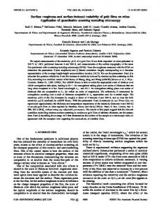
turbine site in Denmark in a spring and a fall campaign in 1994. The experiment comprises two 48 m offshore towers and one tower on the coast on the island of Lolland. The tower used for this study was situated in about 4-m water depth with an upstream fetch of 15– 20 km in a 90 degree sector with upstream water depths of 5–20 m (see Fig. 1). For this paper, we used the lowest sonic anemometer (Solent, 3-component research type) mounted 3 m above MSL. Data were logged as 30-min time series sampled at 20 Hz, which were subsequently subjected to a coordinate transformation to orient the x-axis into the mean wind. A linear trend was removed from the data before the covariances were calculated. The estimated uncertainty on the resulting value of u* is about 10%. The mean wind speed was derived from the lowest cup anemometer at 7 m, measuring mean wind speed with an estimated accuracy of about 2%. The wave gauge was an acoustic device placed on the sea bottom about 30 m west-northwest from the tower, measuring the water level fluctuations eight times per second. Again 30-min time series were logged, and power spectra were calculated by use of FFT. From the spectra three frequencies, f 25 , f 50 , and f 75 , were derived at 25%, 50%, and 75% accumulated variances. Then f 50 was used as a measure of the peak frequency of the spectrum, and BW 5 log10 ( f 75 / f 25 ) then serves as a measure of the widths of the spectral peaks. Rather than computing the peak frequency directly, we chose the statistically more stable way of computing f 50 , which means that we need to assume a model for the spectra to arrive at the correct peak frequency. A JONSWAP model (see section 5) fits the data well with a peak enhancement factor of 1.0 (in the JONSWAP experiment, the mean value for this parameter was found to be 3.3). The dataset There were available 1987 30-min time series from the RASEX experiments, taken at the Vindeby site during spring and fall 1994. From the time series a number of characteristic parameters were computed. The data were sampled at 8 Hz, but a cutoff frequency of 2 Hz was applied to minimize the influence of noise. The available data are: T 50 :

Tm : Tz :

Period of spectrum computed such that 50% of the variance in the spectrum is found on either side of the frequency 1/T 50 . This frequency is slightly larger than the actual peak frequency in our model spectrum. The peak frequency corresponding to the fitted JONSWAP spectrum is computed as f p 5 1/(1.156T 50 ). Mean period of waves 5 m 0 /m1 , where m i is the spectral moment: m i 5 ∫`2` f iS( f ) df. Wave period based on zero crossing frequency 5 (m 0 /m 2 ) 0.5.

VOLUME 28

Hs :

Significant wave height derived as four times the standard deviation of the surface elevations. BW: The bandwidth of the spectrum, defined as BW 5 log10 ( f 75 / f 25 ), where f 25 is the frequency at which the integrated variance is 25% of the total variance and f 75 is the frequency at which the integrated variance is 75%. In other words, 50% of the variance is situated between the two frequencies. This parameter enables us to distinguish between data with two-peaked spectra (very wide) from the single peak spectra that are similar to our model (which has a BW of 0.171). MSL: Water depth to mean sea level (m). U7: Average wind speed (m s21) at an elevation of 7 m above MSL. U15 : Average wind speed (m s21) at an elevation of 15 m. dir 20 : Average wind direction (8N) at an elevation of 20 m. u*2 : Total wind stress (m s21 ) 2 5 sqrt(ûw& 2 1 ûw& 2 ), where 2ûw& is the alongwind stress and ûw& is the stress perpendicular to mean wind. 4. Analysis of RASEX data In this section we present results of the analysis of selected data collected during RASEX. First, we carry out a dimensionless analysis of the problem, next the measured and derived quantities are presented together with an assessment of errors, then the influence of wave age on sea roughness is examined, and finally some inferences are made from the data. a. Dimensionless analysis Any property, A, depending on the interaction between the air and the sea surface can be described generally as A 5 f (wind flow near sea, sea surface).

(4.1)

The wind flow near the sea can be described in its most general form by the following independent parameters: wind 5 f (u*, F a , r a , m a , g, u a , sea surface), (4.2) where u* is the wind friction velocity, F a is the wind direction, r a is the density of air, m a is the dynamic viscosity of air, g is the acceleration due to gravity, and u a is the air temperature. Similarly, the independent parameters describing the sea surface can be listed as sea surface 5 f(H, T, Fw, d, rw, mw, uw, g, z 0s), (4.3) where H is a characteristic wave height (taken as H m0— the significant wave height), T is a characteristic period (taken as T p—the peak period), F w is the wave direction, d is water depth, r w is the density of water, m w is the dynamic viscosity of water, u w is the temperature of the

SEPTEMBER 1998

1705

JOHNSON ET AL.

FIG. 1. The RASEX site at Vindeby. From left to right: Denmark–Langeland/Lolland–closeup of site. The filled circles are wind turbines, the triangles are the two 48-m offshore lattice towers and the coast tower. The tower used for this study was situated west of the wind farm (SMW). Distances on the two leftmost figures are in kilometers, on the closeup in meters.

water, g is the acceleration due to gravity, and z 0s is the background sea roughness (sea roughness in the absence of waves). Thus, Eq. (4.1) can be rewritten as A 5 f (u*, F a , r a , y a , g, u a , H m0 , T p, F w , d,

r w , y w , u w , z 0 s ),

(4.4)

where m has been replaced by the kinematic viscosity, n 5 m/r. Now, using ra , g, and u* as repeaters, the following dimensionless form of Eq. (4.4) can be obtained:

1

2

1

2

u3 gH m0 gT p gd r w u 3 gz 0s A˜ 5 f F a , * , u, 2 , , F wi 2 , , * , u w , 2 gy a u* u* u* r a gy w U* or

gH m0 gT p gd gz 0 s u3 u3 rw A˜ 5 f , , 2 , 2 , ua, uw, Fa, Fw, * , * , . 2 u* u* u* u* gy a gy w r a (4.5) Now, we introduce a number of simplifications. First, we assume locally generated waves implying a relationship between H m0 and T P (for instance, Toba’s relationship), thus, we can drop one of H m0 and T P . Next,

we combine the second and third terms in the phase celerity c p using the dispersion relationship. This assumes that the only influence of water depth is in the modification of the phase celerity. Obviously, this excludes situations where depth-induced breaking is important. Next we assume the sea surface is completely smooth in the absence of waves and drop the fourth term. Last we assume rough turbulent flow conditions at the air–sea interface (dropping the ninth and tenth terms). Now, Eq. (4.5) can be rewritten as cp A˜ 5 f , u , u , F , F , r /r . (4.6) u* a w a w w a In Eq (4.6) u a and u w contribute to the momentum exchange at the air–sea interface due to stratification, thus for neutrally stratified flows (in which case the air– sea temperature difference is small), they can be dropped from Eq. (4.6). Also, if we limit ourselves to cases where the wind and waves are nearly in the same direction, F a and F w can also be dropped from Eq. (4.6). Lastly, we consider situations with constant r w /r a , and drop this term. Hence Eq. (4.6) can be expressed as A˜ 5 f (c p /u*). (4.7) If A˜ is the dimensionless sea roughness at the air–sea interface, Eq. (4.7) can be written as

1

2

1706


gz 0 5 f (c p /u*). u*2

(4.8)

From the preceding paragraphs, Eq. (4.8) shows that the dimensionless sea roughness (or Charnock parameter) is a function of wave age only if the following conditions are satisfied: 1) locally generated wind waves, 2) rough turbulent flow conditions at the air–sea interface, 3) neutrally stratified conditions, 4) waves and wind in nearly the same direction, and 5) no background sea roughness (i.e., sea is smooth in the absence of waves). b. Considerations for selecting a data subset for analysis It is intended to investigate the dependence of the sea roughness on wave age. Based on the dimensionless analysis in the preceding section, a number of conditions must be satisfied in order for Eq. (4.8) to be valid. This therefore imposes the necessary considerations for selecting a data subset for analysis. These considerations are 1) locally generated waves, in which there is a definite relationship between H m0 and T P ; 2) rough turbulent flow conditions at the air–sea interface (following Toba et al. 1991), defined as cases with u*z 0 /n . 2.3);



2 ln 11 12F  C5 25z /L,

21 m

2

1 ln

1

2

where F m 5 (1 2 16z/L)21/4 for z/L , 0; and L is the Monin–Obukhov length. Thus, using the measured wind speed, wind friction velocity, and Monin–Obukhov length, the equivalent neutral wind speed at a given elevation is obtained. For this analysis, the neutral wind speed at 7-m elevation is corrected to 10-m elevation using the 1/7 power law. Thus U10n 5 U7n

3) neutrally stratified situations (or equivalent neutral parameters); and 4) wind and waves in nearly the same direction, which is assumed to be the case for locally generated waves with F a 5 2708N 6 22.58. c. Measured and derived quantities In order to satisfy the third condition in section 4b, the measured winds were converted to equivalent neutral winds. In the presence of stratification, the wind profile can be written as in Eq. (4.9) following the Monin–Obukhov similarity theory: U(z) 5

1 2 10 7

1/7

.

(4.13)

Given the neutral wind speed at 7-m elevation and the measured friction velocity, the sea roughness z 0 , is calculated from Eq. (4.10). The neutral drag coefficient C dn is calculated as C dn 5 u*2 /U 210n, (4.14) while the phase speed at peak frequency c p is calculated using the measured water depth and peak frequency in the linear dispersion relationship.

1

2

u* z ln 2 C , k z0

(4.9)

where C is a stratification function. Now, defining the equivalent neutral wind, U n (z) as U n (z) 5

u* z ln , k z0

(4.10)

Eqs. (4.9) and (4.10) can be combined to give U n (z) 5 U(z) 1 Cu*/k. (4.11) Following Geernaert et al. (1988) the stratification function is given as

1 1 F22 m 2 2 tan 21 (F21 m ) 1 p /2, 2



VOLUME 28

z /L , 0

(4.12a)

z /L $ 0,

(4.12b)

d. Data results Table 1 presents the measured and derived data satisfying the conditions described in section 4b. A plot of the dimensionless wave energy (1/16)(gH m0 /u*2 ) 2 versus the dimensionless frequency vpu*/g is shown in Fig. 2 for data runs satisfying the rough flow conditions (u*z 0 /n . 2.3) and winds from 2708 6 22.58. The dotted line in Fig. 2 is the relationship suggested by Toba (1978). Figure 2 shows a unique relationship between H m0 and T P , as assumed in section 4b. Now, in order to investigate the functional form of Eq. (4.8), the Charnock parameter, zch (5gz 0 /u*2 ) is plotted against the inverse wave age (u*/c p ) in Fig. 3. A weak trend of increasing zch with wave age can be observed. This trend is opposite to the widely believed trend of zch decreasing with wave age (Maat et al. 1991; Smith et al. 1992; Donelan 1990; Donelan et al. 1993). We note, however, that Toba et al. (1990) suggested the type of trend indicated in Fig. 3 (dashed line by Toba et al. 1990).

SEPTEMBER 1998

1707

JOHNSON ET AL.

Before carrying out any further analysis, it is important to assess the potential errors in the zch derived from measurements. This is the subject of the section below. e. Errors Recall from Eq. (4.10) that the sea roughness z 0 is calculated as z0 5

10 . exp(kU10 n /u*)

(4.15)

Now, suppose there is an error in k, U10n, and u*, given as Dk/k, DU10n /U10n , Du*/u* respectively, then the corresponding error in z 0 (Dz 0 /z 0 ) is given as

5

2k /ÏC d n Dz 0 1 1 5 exp z0 (1 1 Du*/u*) 3

[

1 21 2

]6

DU10 n Dk Dk DU10 n Du* 1 1 2 . U10 n k k U10 n u* (4.16)

The corresponding error in the Charnock parameter (Dzch /zch ) is given as Dz ch Dz 0 /z 0 1 1 115 . z ch (1 1 Du* /u*) 2

(4.17)

Lastly, the error in wave age can be written as D(c p /u*) Dc p /c p 2 Du*/u* 5 . c p u* 1 1 Du*/u*

(4.18)

Now, from section 3, the overall error in u* is about 610%, while the error in U10 is generally much smaller, ,2%. Similarly, the errors in water depth, peak frequency, and thus phase celerity c p , are small. Assuming k equals 0.4 and C dn is 1.5 3 1023 (approximate mean value for this data), and negligible errors in all other parameters except u*, then a 610% error in u* implies that zch can vary between 0.39 and 2.13 of the true value. Assuming the mean value of all the data is the true value, then one can plot the corresponding error bars for 610% error in u* as shown in Fig. 3. The corresponding error in c p /u* is approximately 69%. It is noted from Fig. 3 that most of the data points lie within the 610% error band for u* . In other words, the apparent trend in the data is contained within the error band. In this situation, one cannot talk of a trend in the data. Rather, we will use the mean value of z ch to characterize the dimensionless roughness from this set of measurements. Investigation into the individual field datasets presented in Fig. 2 of Donelan et al. (1993) indicates that for each dataset most of the points are contained within a 610% error in u * (see Figs. 4a–d). Now, since errors of 610% in u* are not unusual for conventional measurements, this indicates that it is difficult to infer trends from individual datasets.

Fortunately, the different datasets are collected in different wave age intervals. Hence, by using the mean values of z ch corresponding to the mean value of wave age, one can plot all datasets together and infer a trend from the composite dataset. This plot is shown in Fig. 5 and it indicates a trend of decreasing zch with wave age. Note that in carrying out this composite analysis, we have assumed that all the datasets satisfy the four conditions described in section 4b above. A least squares fit of the composite data in Fig. 5 gives zch 5 1.89(c p /u*)21.59 .

(4.19)

This expression is obtained in the wave age range 7 # c p /u* # 26. Figure 6 shows a plot of all the data used in the analysis with the regression line [Eq. (4.19)]. It is seen that the regression line describes the general trend in the data reasonably. Thus, it can be concluded that there is experimental evidence that the sea roughness depends on wave age. The next question is whether existing theories can be used to model this behavior. This question is examined in section 5. In section 4f, we discuss the question of self-correlation. f. Problems with self-correlation in scaling with u* The question of spurious self correlation has been addressed by Smith et al. (1992). They obtained two conditions for negligible self-correlation in a relationship of the type: zch 5 b(c p /u ) a . These conditions are * var (lnu*a ) K var (lnz ch )

(4.20)

var(lnu*) K var (lnc p ),

(4.21)

where var( · ) is the variance of the variable within parentheses. Using the logarithmic profile, z ch 5 (10g/u*2 ) exp(2kU10 /u*), thus var(lnz ch ) 5 var(lnu*2 ) 1 var(2kU10 /u*), (4.22) where negligible covariance between lnu*2 and U10 /u* was assumed. Now, Kahma and Calkoen (1994) obtained the following expression for fetch-limited wave growth in deep water:

v p u* gX 5 3.08 2 g u*

1 2

20.27

,

(4.23)

where v p 5 2p/T p and X is the upwind fetch. Using Eq. (4.23), the wave celerity at peak frequency, c p , is u 0.46 X 0.27 cp 5 * . 3.08g

(4.24)

Thus var(lnc p ) 5 var(lnu*0.46) 1 var(lnX 0.27 ).

(4.25)

1708


VOLUME 28

TABLE 1. Measured and derived data (wind direction 5 270 6 22.5, u*z0/n .2.3). Run name (YYMTDepth DDHHMM) (m) 9410060456 9410110409 9410301114 9410141040 9410150822 9410150852 9410151122 9410171526 9410151052 9410140246 9410171556 9410150922 9411021111 9410120222 9410131816 9411020831 9411020959 9410130032 9410041204 9410041834 9410041404 9410041604 9410030700 9410130102 9410041704 9410041734 9410041634 9410130302 9410040849 9410041134 9410041019 9410041804 9410010234 9411012231 9410050504 9411020001 9410041934 9411012201 9410040719 9411012331 9410040749 9411012031 9411012301 9410040919 9410050404 9410010304 9411012131 9410042004 9410042234 9410050604 9411012001 9411012101 9410050634 9410042204 9410042134 9410040507 9410040949 9410042104 9411011931 9410050034 9411011901 9410041434 9410050104

3.71 3.89 3.93 3.71 3.97 4.00 3.99 3.72 4.02 3.65 3.71 4.03 3.94 3.60 3.81 3.72 3.87 3.80 3.95 3.62 3.83 3.62 3.44 3.75 3.58 3.57 3.59 3.68 3.92 3.97 3.98 3.59 3.37 3.59 3.50 3.60 3.70 3.59 3.82 3.60 3.85 3.55 3.59 3.95 3.53 3.35 3.58 3.77 3.88 3.51 3.52 3.57 3.53 3.86 3.84 3.74 3.96 3.82 3.47 3.81 3.44 3.75 3.78

Hm0 (m)

Tp (sec)

0.187 0.218 0.222 0.270 0.274 0.275 0.279 0.291 0.291 0.299 0.309 0.309 0.324 0.341 0.347 0.393 0.425 0.427 0.441 0.442 0.450 0.452 0.456 0.459 0.462 0.464 0.483 0.483 0.487 0.492 0.492 0.493 0.496 0.496 0.503 0.504 0.504 0.507 0.510 0.515 0.515 0.521 0.523 0.524 0.526 0.527 0.528 0.528 0.528 0.530 0.534 0.537 0.547 0.548 0.552 0.554 0.559 0.560 0.561 0.569 0.570 0.579 0.586

2.10 2.13 2.28 2.66 2.52 2.50 2.65 2.42 2.75 2.72 2.52 2.67 2.88 2.74 2.72 2.91 3.07 3.03 3.14 2.96 2.91 2.86 2.84 3.03 3.04 2.99 3.04 3.17 3.31 3.26 3.29 3.11 2.90 3.13 3.10 3.25 3.05 3.07 3.34 3.09 3.33 3.10 3.29 3.31 3.33 3.16 3.17 3.13 3.36 3.28 3.07 3.31 3.27 3.26 3.26 3.44 3.48 3.27 3.12 3.55 3.13 3.25 3.57

U7 dir20 (m s21) (deg) 4.09 3.79 6.40 4.50 5.46 5.17 5.04 5.79 4.50 4.18 5.06 5.55 4.96 6.05 5.59 6.87 6.26 8.47 8.53 9.18 10.42 10.13 9.93 8.47 8.81 9.14 9.56 8.20 8.37 8.68 9.03 9.98 12.50 10.50 9.20 10.03 8.90 10.89 9.40 10.40 8.68 11.41 10.74 8.15 9.77 11.74 10.39 8.86 9.15 8.86 11.74 11.21 8.81 8.97 8.73 9.27 8.86 9.47 12.06 10.04 12.95 8.92 10.38

249 261 256 261 269 274 286 277 286 269 291 285 285 257 251 266 276 279 262 276 282 275 259 282 265 271 281 289 272 267 265 263 248 262 284 268 283 262 279 263 275 261 264 276 280 257 260 280 276 289 257 261 290 272 273 290 264 277 253 281 253 269 278

ûw&

^vw&

z/L

20.0281 20.0227 20.0619 20.0292 20.0474 20.0533 20.0479 20.0507 20.0306 20.0274 20.0417 20.0579 20.0414 20.0507 20.0359 20.0722 20.0569 20.1025 20.1061 20.1369 20.1747 20.1304 20.0777 20.0997 20.1076 20.1267 20.1406 20.1151 20.1143 20.1130 20.1246 20.1743 20.2128 20.1561 20.1158 20.1606 20.1192 20.1848 20.1288 20.1606 20.1213 20.1683 20.1662 20.0893 20.1313 20.1942 20.1415 20.1152 20.1385 20.1162 20.2052 20.1689 20.1147 20.1050 20.1106 20.1216 20.1412 20.1382 20.2312 20.1425 20.2631 20.1509 20.1530

20.0103 20.0115 20.0098 20.0173 20.0128 20.0078 20.0174 20.0582 20.0179 20.0198 20.0145 20.0219 20.0088 20.0165 20.0297 20.0035 0.0003 0.0058 20.0167 20.0605 20.1055 20.0794 20.2107 20.0058 20.0382 20.0495 20.0723 20.0075 20.0335 20.0291 20.0392 20.0796 20.0506 20.0433 20.0352 20.0156 20.0189 20.0563 20.0266 20.0437 20.0487 20.0510 20.0478 20.0765 20.0431 20.0658 20.0370 20.0427 20.0689 0.0012 20.0583 20.0567 0.0118 20.0869 20.0512 20.0143 20.0562 20.0389 20.0497 20.0302 20.0745 20.0674 20.0662

0.0742 20.1921 20.0321 20.1114 20.2078 20.1667 20.0848 20.0769 20.2360 20.2462 20.0894 20.1079 0.0328 20.0215 0.0233 20.0305 20.0181 20.0633 20.1201 20.0921 20.0951 20.1376 20.0061 20.0570 20.1067 20.1148 20.0950 20.0365 20.1196 20.1363 20.1316 20.0850 20.0154 20.0155 20.1326 20.0205 20.1271 20.0108 20.1562 20.0186 20.1381 20.0103 20.0133 20.1420 20.1214 20.0213 20.0121 20.1394 20.1064 20.1535 20.0078 20.0132 20.1517 20.0848 20.1089 20.1273 20.0873 20.1074 20.0056 20.1099 20.0154 20.0308 20.1054

u* Cp U10n (m s21) (m s21) (m s21) 0.17 0.16 0.25 0.18 0.22 0.23 0.23 0.28 0.19 0.18 0.21 0.25 0.21 0.23 0.22 0.27 0.24 0.32 0.33 0.39 0.45 0.39 0.47 0.32 0.34 0.37 0.40 0.34 0.35 0.34 0.36 0.44 0.47 0.40 0.35 0.40 0.35 0.44 0.36 0.41 0.36 0.42 0.42 0.34 0.37 0.45 0.38 0.35 0.39 0.34 0.46 0.42 0.34 0.37 0.35 0.35 0.39 0.38 0.49 0.38 0.52 0.41 0.41

3.25 3.29 3.51 3.99 3.84 3.81 4.00 3.69 4.13 4.05 3.82 4.03 4.27 4.07 4.07 4.27 4.46 4.40 4.55 4.30 4.29 4.20 4.15 4.40 4.37 4.33 4.38 4.51 4.69 4.66 4.69 4.44 4.20 4.46 4.41 4.56 4.41 4.41 4.70 4.42 4.69 4.42 4.60 4.70 4.61 4.42 4.49 4.50 4.73 4.57 4.39 4.60 4.56 4.64 4.63 4.76 4.85 4.64 4.42 4.86 4.42 4.60 4.86

4.14 4.17 6.80 4.88 6.01 5.68 5.44 6.25 4.98 4.64 5.46 6.03 5.14 6.41 5.82 7.30 6.63 9.07 9.24 9.92 11.27 11.01 10.48 9.06 9.52 9.91 10.33 8.74 9.09 9.44 9.82 10.78 13.22 11.11 9.98 10.63 9.66 11.50 9.87 11.01 9.46 12.05 11.35 8.89 10.58 12.44 10.98 9.64 9.92 9.65 12.39 11.85 9.60 9.67 9.45 10.05 9.57 10.25 12.72 10.86 13.70 9.50 11.22

z0 (m)

1000Cdn

0.00069 0.00029 0.00019 0.00025 0.00020 0.00056 0.00065 0.00123 0.00026 0.00041 0.00031 0.00062 0.00046 0.00015 0.00021 0.00019 0.00015 0.00012 0.00013 0.00035 0.00046 0.00013 0.00144 0.00011 0.00013 0.00022 0.00031 0.00034 0.00027 0.00016 0.00019 0.00053 0.00012 0.00016 0.00010 0.00025 0.00015 0.00028 0.00019 0.00020 0.00029 0.00010 0.00018 0.00031 0.00011 0.00017 0.00010 0.00017 0.00042 0.00012 0.00022 0.00013 0.00012 0.00028 0.00020 0.00010 0.00054 0.00020 0.00029 0.00011 0.00028 0.00088 0.00017

1.7432 1.4652 1.3535 1.4270 1.3604 1.6712 1.7191 1.9735 1.4313 1.5697 1.4801 1.7042 1.6051 1.2970 1.3758 1.3560 1.2956 1.2474 1.2575 1.5216 1.6058 1.2596 2.0457 1.2175 1.2593 1.3857 1.4813 1.5117 1.4424 1.3101 1.3558 1.6500 1.2514 1.3131 1.2141 1.4281 1.2936 1.4596 1.3509 1.3721 1.4611 1.2116 1.3416 1.4879 1.2334 1.3246 1.2138 1.3222 1.5718 1.2473 1.3899 1.2690 1.2522 1.4576 1.3647 1.2120 1.6584 1.3669 1.4622 1.2361 1.4564 1.8328 1.3233

SEPTEMBER 1998

1709

JOHNSON ET AL. TABLE 1. (Continued).

Run name (YYMTDepth DDHHMM) (m) 9410050004 9410042304 9410040607 9410050726 9410040637 9411011301 9411011801 9411011831 9411011631 9411011331 9411011601 9411011701 9410031752 9411011431 9411011401 9411011501 9410031822

3.83 3.88 3.76 3.58 3.78 3.65 3.40 3.43 3.42 3.59 3.42 3.41 3.69 3.52 3.56 3.48 3.70

Hm0 (m)

Tp (sec)

0.586 0.586 0.589 0.592 0.597 0.603 0.610 0.622 0.632 0.634 0.636 0.640 0.666 0.672 0.675 0.691 0.711

3.40 3.35 3.49 3.44 3.51 3.32 3.21 3.23 3.23 3.23 3.24 3.19 3.87 3.33 3.42 3.29 3.62

U7 dir20 (m s21) (deg) 9.77 10.02 8.60 9.02 8.83 13.62 14.32 14.07 14.90 14.30 14.33 14.28 9.53 15.49 15.44 15.05 12.57

277 283 286 292 286 248 248 253 249 248 248 248 287 248 248 248 291

ûw&

^vw&

z/L

20.1479 20.1332 20.1069 20.1266 20.1146 20.3233 20.4028 20.3394 20.3978 20.3523 20.3868 20.3742 20.1322 20.4602 20.4512 20.4537 20.2584

20.0314 20.0377 20.0183 0.0092 20.0292 20.0930 20.1119 20.0883 20.1348 20.0950 20.1067 20.0923 20.0530 20.1237 20.1463 20.1422 20.0493

20.1109 20.1108 20.1315 20.1362 20.1262 20.0022 20.0113 20.0150 20.0112 20.0046 20.0105 20.0144 20.1676 20.0079 20.0092 20.0077 20.0962

Using Eqs. (4.22) and (4.25) and the identity, var(cY) 5 c 2 var(Y) (where c is a constant and Y is a random variable), Eqs. (4.20) and (4.21) can be simplified to a2 K 4 1

var (2kU10 /u* ) var (lnu*)

1 K 0.212 1 0.073

var (lnX ) . var (lnu*)

(4.26) (4.27)

In general, Eq. (4.26) is satisfied if |a| , 2 (which is usually the case), while Eq. (4.27) is not necessarily satisfied. In fact, for a given site where the fetch varies

FIG. 2. Illustration of correlation between the dimensionless energy and peak frequency. The crosses represent the data, while the dotted lines is the relationship suggested by Toba (1978).

u* Cp U10n (m s21) (m s21) (m s21) 0.39 0.37 0.33 0.36 0.34 0.58 0.65 0.59 0.65 0.60 0.63 0.62 0.38 0.69 0.69 0.69 0.51

4.75 4.72 4.80 4.71 4.82 4.63 4.48 4.50 4.50 4.54 4.51 4.46 5.03 4.61 4.69 4.57 4.87

10.58 10.83 9.33 9.81 9.58 14.35 15.14 14.89 15.75 15.08 15.14 15.11 10.42 16.35 16.31 15.89 13.58

z0 (m)

1000Cdn

0.00019 0.00009 0.00012 0.00017 0.00014 0.00051 0.00086 0.00043 0.00060 0.00046 0.00070 0.00059 0.00016 0.00077 0.00077 0.00099 0.00025

1.3511 1.1806 1.2446 1.3195 1.2883 1.6348 1.8243 1.5820 1.6936 1.6056 1.7499 1.6880 1.3129 1.7821 1.7835 1.8835 1.4263

slowly Eq. (4.27) will not be satisfied. Thus, self-correlation has some influence on results from a single site, as was found by Smith et al. (1992) for the HEXOS measurements. However, if the results from several sites with different fetches are aggregated together as done in this paper, var(lnX) is no longer close to zero, making it possible that Eq. (4.27) is satisfied. In this case, the influence of self-correlation due to scaling with u* is significantly reduced. This provides an additional reason

FIG. 3. Scatterplot of the Charnock parameter and inverse wave age for the RASEX dataset (diamonds). The dashed line is the relationship suggested by Toba et al. (1990), while the dash–dot line is the mean value for the Charnock parameter.

1710


VOLUME 28

FIG. 4. Scatterplot of the Charnock parameter and inverse wave age for datasets compiled in Donelan et al. (1993). The dash–dot line is the mean value for the Charnock parameter.

why care must be taken in analyzing data from a single site. 5. Comparison with other roughness models Below we discuss the comparisons between the measured stress values from the dataset and results derived

from two different descriptions of the sea roughness, the one being Charnock expression, as depicted by Eq. (4.8). The second expression was derived by Hansen and Larsen (1997), who obtained an expression for the sea surface roughness by considering the waves as roughness elements in the sense of Lettau (1969), and combining this with Kitaigorodskii’s idea about the in-

SEPTEMBER 1998

1711

JOHNSON ET AL.

FIG. 5. Scatterplot of the mean Charnock parameter from different datasets and inverse wave age. The full line is the least squares best fit line.

FIG. 6. Scatterplot of the Charnock parameter from different datasets and inverse wave age. The full line is the least squares best fit line from Fig. 4.4. 

dividual roughness elements being wavelets moving with their individual phase speeds. Kitaigorodskii (1970) noticed that the wavelets, considered as roughness elements, moved with their phase speed c relative to a stationary coordinate system. Since the wind profile in this system and any other inertial coordinate system moving with c should be given by the same logarithmic profile, the relation between the roughness effect of the wavelet in the stationary system z 0 , and in the moving coordinate system z c , should be given by z 0 5 z c exp(2kc/u*),

(5.1)

where z 0 is the roughness experienced by the wind, while z c is the corresponding roughness in a coordinate system moving with the phase speed of the wave c, k is the von Ka´rmań constant, and u* is the friction velocity. The value for z c for a field of roughness elements is estimated from Lettau’s (1969) relation for roughness elements: z c 5 a L hX/A,

(5.2)

where a L is a coefficient of order unity, h is the height of the element, X its cross-wind area, and A is the horizontal area available to each element. Identifying h in Eq. (5.2) with the wave height (twice the amplitude a) and X/A with ak/p (where k is the wavenumber), Hansen and Larsen transform Eq. (5.2) to a form appropriate for wavelets:

 

a L hX/A 5

zc 5



2 2 a a 2 k 5 a L s 2 k21 , p L p

s . s0

(5.3a)

0



s # s0 .

(5.3b)

In Eq. (5.3), it is implied that only wavelets with a steepness, s (s 5 ak), larger than s 0 can create flow separation and thereby qualify as roughness elements. The value of s 0 is found to be between 0.25 and 0.3. To interpret Eq. (5.3) it is assumed that the roughness wavelets constitute a random superposition of harmonic components in a narrow wavenumber band, that is, essentially of one wavenumber, ^k&, defined by

E E

`

^h 2 &^k& 5

k9F(k9)k9 dk9

k `

^h 2 & 5

k

(5.4)

E

`

k9F(k9)k9 dk9 5

S(v9) dv9,

(5.5)

v

where F(k) is the one-dimensional wavenumber spectrum of the surface displacement h(x, t) and S(v) is the omnidirectional frequency spectrum. To derive the average ^z c & from a given ^k&, Hansen and Larsen (1997) argue that the steepness s in Eq. (5.3) essentially follows an exponential distribution in the normalized variable, y 5 s 2 /(2^h 2 &^k& 2 ). Using this exponential distribution and averaging z c over all steepness values larger than s 0 , the average contribution to z c , ^z c &, from a narrow k interval around ^k& was found as function of ^k&.

1712


FIG. 8. Bandwidth of RASEX wave spectra.

FIG. 7. Distribution of significant wave heights for the RASEX dataset.

2 ^z c & 5 a L ^h 2 &xe2x ^k&, p

(5.6)

where x is the normalized critical steepness: s02 x5 . 2^h 2 &^k& 2

(5.7)

The contribution to ^z c & from an infinitesimal wavenumber interval dk is found by differentiating ^h 2 &^k& in Eq. (5.6) using Eq. (5.4) to yield 2 d^z c & 5 a L xe2x kF(k)k dk . p

(5.8)

Equation (5.8) is finally combined with Eq. (5.1) to yield the contribution to z 0 from and infinitesimal wavenumber interval dk: dz 0 5 a L

2 2x 2kg/^v&u* 2 xe e v S(v) dv, pg

VOLUME 28

tabulating the spectral moments of the waves and doing the integrations at a certain number of fixed frequencies. The necessary steps from measurements to resulting roughness lengths are then 1) Find a suitable spectral model that fits the data sufficiently well. 2) Screen the data to exclude unwanted wind directions, situations with ‘‘strange’’ spectra and low wind speeds with large measurement errors. 3) Compute roughness lengths from spectral model. 4) Compare wind stress derived from roughness lengths of ‘‘3’’ and mean wind speed (log-windprofile) with directly measured windstress. 5) If there are systematic differences in ‘‘4,’’ then go back to ‘‘3,’’ multiply the roughness lengths with a constant and check differences again. b. Model wave spectrum

(5.9)

where x and ^v& are to be evaluated by use of Eqs. (5.4) and (5.5) with v 2 5 gk, when needed. Subsequently integrating over v, using the Kitaigorodskii form of S(v), Hansen et al. (1990) and Hansen and Larsen (1997) find the contribution to z 0 from different frequencies for different sea states. The behavior is similar, but not identical, to that of the Kitaigorodskii model (Kitaigorodskii and Volkov 1965; Kitaigorodskii 1970) and has the advantage that the empirical coefficient, a L , in Eq. (5.9) is of order unity as opposed to the other models available for the sea roughness. a. From wave spectrum to roughness length The derivation of roughness lengths from the measured wave spectra is quite time consuming and somewhat complicated because of the integration involved in the calculation of Eq. (5.9). Instead, we have chosen a simpler method in which a model wave spectrum is fitted to the data using only measured values of peak frequency f p and the measured significant wave height H s . The computations can then be greatly simplified by

The model chosen is a JONSWAP-type spectrum (Hasselmann et al. 1973):

[

S( f ) 5 a P g 2 (2p)24 f 25 exp 2

12

5 f 4 fp

24

]

gG,

(5.10)

where

1

G 5 exp 2

( f 2 fp)2 , 2s 2 f 2p

2

where a P is the Phillips constant, g is acceleration of gravity (m s21 ), f is frequency (Hz), f p is peak frequency, g is peak enhancement factor, and s is 0.07 for f , f p , 0.09 for f . f p . We used the somewhat simplified version of Eq. (5.10) with g 5 1.0. As shown below the simplified model fits the data well. The distribution of available time series as a function of wave height is shown in Fig. 7. To check the applicability of the model we compared measured spectral bandwidths to model bandwidth (Fig. 8). We see that for a wide range of wave heights we get good correspondence between model and data. As expected, the waves with small amplitudes also show spectra that are

SEPTEMBER 1998

1713

JOHNSON ET AL.

FIG. 9. Comparison between ratios of measured characteristic wave periods and model derived wave periods. Model values are shown as horizontal lines.

wider than the model; in some cases clear two-peaked behavior was seen. The measured wave periods are compared with the model parameters in Fig. 9, from which we can see that there seems to be some systematic change of the peak shape with T p increasing slightly for increasing wave height compared to the model, whereas the periods based on the spectral moments (dominated by higher frequencies) are very well modeled. c. Screening of data The data used in the analysis here were screened according to the following criteria: Wind direction: Only directions with an undisturbed fetch of 10–20 km were used (the longest usable fetch from the RASEX experiment), that is, 2408– 3308. Wave spectra: Only data with spectra with a bandwidth BW , 0.3 were used. Wind stress: Only data with measured stress .0.0025 m 2 s22 (friction velocity u* . 0.05 m s21 ) were used. Wind speed: Because of the sampling method applied, the mean wind speeds measured by the cup anemometers were unreliable for speeds ,2 m s21 , which were then excluded. Wave height: Significant wave heights ,0.1 m were excluded. Roughness: Roughness lengths computed from the wave spectra with values z 0 , 10210 m were not used. After screening for spectral widths, wind stress, wave height, and roughness about 1500 datasets remained. Selecting the proper wind direction sector left us with 576 30-min time series that were used. d. Wind stress The friction velocities were computed from the roughness lengths inferred from the wave spectra using

FIG. 10. Comparison between measured u (52|ûw&| 0.5 ) and u * derived from the log wind profile and z 0 from the wave spectra.*

Eq. (5.9), the mean wind speed at a height of 7 m in the logarithmic profile. The computed friction velocities were compared with the alongwind component of the wind stress measured at 3 m, that is, u*2 5 ^2u9w9&. A least squares fit was calculated and the roughness lengths were multiplied by a constant in order to obtain a 1:1 relation between the measured and calculated values. The value of the constant that was used was 5.0. The fit was forced through 0. The results are shown in Fig. 10, from which we can see that the correspondence is very good with the spreading somewhat increasing at friction velocities higher than 0.4 m s21 . We can also derive the friction velocity from the Charnock relation u2 z0 5 A * , g

(5.11)

where we can use the logarithmic wind profile to derive an implicit equation for u*, that can easily be iterated using a measured value of the wind speed U.

1 2

z exp 2

Uk u2 5 A *, u* g

(5.12)

where z is the height above the surface, U the mean wind speed, and k the von Ka´rmań constant (50.4). The resulting friction velocities were compared with the measured friction velocities and the calculated values were adjusted to a 1:1 relationship by adjusting the Charnock constant A to a value of 0.018 (see Fig. 11), which as expected for this coastal site is on the high side of the range found in the literature, 0.011 , A , 0.018 (among others, Wu 1980; Garratt 1977; Smith and Banke 1975; Walmsley 1988). Finally, in Fig. 12 we have compared the bin-aver-

1714


FIG. 11. Comparison between measured friction velocity and the friction velocity derived using the Charnock relation with a Charnock constant of 0.018.

aged values of the two different estimates of friction velocities, and we can see that the Hansen and Larsen method gives rise to slightly larger variations, and some deviations from the straight line above 0.4 m s21. The Charnock u* shows small deviations from the straight line at small friction velocities (the least squares fit showed an offset of 0.01 m s21 . e. The Charnock ‘‘constant’’

VOLUME 28

FIG. 12. Binned averages of the data from Figs. 10 and 11. The vertical bars signify 61 standard error on the mean value.

zchu*2 ,Charnock /u*2 ,measured . Here, we see a systematic overprediction of u*2 for the old waves (low inverse wave age). For the younger waves (and fully rough flow), this overprediction is diminished, since the mean trend tends toward 0.018 (the value for zch ). When we are only interested in predicting the wind stress, then we seem to get slightly better results by using a simple Charnock relation, at least for a relatively narrow range of wave ages. On the other hand, we know from the aggregation of experimental results from different sites (Fig. 5) that there seems to be a strong in-

The variation of the Charnock constant A in Eq. (5.11) is plotted in Fig. 13 as a function of inverse wave age. Here we have used the z 0 values calculated from the wave spectra and the directly measured u*. Furthermore, the data have been subdivided into classes of different flow regimes using the method of Kraus and Businger (1994): Aerodynamically smooth flow: u* , 0.11 m s21 Transition flow: 0.11 m s21 , u* , 0.265 m s21 Fully rough flow: 0.265 m s21 , u*. This classification is based on a roughness Reynolds number (u*z 0 /n ) in which z 0 is replaced by the Charnock value. Obviously smooth flow is most often found in cases with old waves and rough flow in situations with younger, developing waves. We observe a systematic variation of gz 0 /u*2 with increasing values for decreasing wave age as discussed in section 4. If instead of using the z 0 values derived using Hansen and Larsen we use the z 0 values from the Chamock relation, we see a quite different relation as seen in Fig. 14. This figure shows how well u*2 is predicted using the Charnock relation, since gz 0 /u*2 is the same as

FIG. 13. Charnock constant plotted as a function of inverse wave age. The z 0 values were derived from the wave spectra.

SEPTEMBER 1998

JOHNSON ET AL.

FIG. 14. As in Fig. 13 only here z 0 was derived from the Charnock relation.

crease of gz 0 /u*2 with decreasing wave age over a wide range of wave ages, which is quite nicely reproduced by the Hansen and Larsen method. Hence, the Charnock method is good for a limited range of wave ages if you can guess the value of the Charnock constant, but the spectral method seems to give a more correct picture in the sense that it is capable of reproducing the variation of the Charnock constant with wave age. Finally, in Fig. 15, we have overlaid the binned results from the Charnock method with the results from the Hansen and Larsen method, where the latter has been subdivided into three different flow regimes. It seems that the average of the curve for the rough flow is consistent with the Charnock results. Furthermore, the Hansen and Larsen method qualitatively reproduce the trend of the Charnock parameter obtained from aggregating various field datasets. Further investigations on the use of existing theories for air–sea momentum flux and implications for wave modeling at the RASEX site was made using WAM cycle 4 model (see Johnson et al. 1997, submitted to J. Oceanic Atmos. Technol.). In that paper, the use of Janssen’s theory in the WAM model, and its applicability at the RASEX site, is discussed at length. 6. Summary and conclusions 1) Dimensionless analysis of the air–sea interaction problem yields a relationship between the dimensionless sea roughness and wave age under specific conditions. 2) Using a selected dataset from RASEX satisfying the conditions in (1), a weak trend of increasing dimensionless roughness with wave age was observed.

1715

FIG. 15. Bin-averaged values from Fig. 5.7 with z 0,WAVE values subdivided into different flow regimes. The vertical bars signify 61 standard error on the mean. The thick line is Eq. (4.19).

3)

4)

5) 6)

However, error analysis indicates that measurement errors of about 10% in u* makes it difficult to conclude on the trend in zch using measured data from a particular dataset. This conclusion was found to be equally valid for other field datasets compiled in Donelan et al. (1993). It was also found that selfcorrelation plays a role in the trend observed from data from a single site. Analysis of the mean dimensionless sea roughness (Charnock parameter) from the field datasets mentioned in 2) gives a trend of decreasing Charnock parameter with wave age. The fitted relationship is zch 5 1.89(C p /U*)21.59 . This relationship establishes the mean trend in the variation of dimensionless sea roughness with wave parameters under the conditions identified in 1) for field data. The wave-dependent sea roughness expression of Hansen and Larsen (1997) was found to reproduce the measured friction velocities in RASEX quite well. Furthermore, it qualitatively reproduced the trend of the Charnock parameter obtained by combining many field datasets. A constant Charnock parameter of 0.0180 was found to adequately reproduce measured friction velocities in the RASEX experiment. From the above results, we conclude that there is evidence that a wave-age-dependent sea roughness is necessary to explain the variation of sea roughness over a wide range of wave ages. Thus, for largescale models, a wave-age-dependent sea roughness models would be necessary. However, for a relatively small range of wave ages, typical of a given site (or a limited area study), a constant Charnock parameter

1716


representative of the typical wave age at the site can be used. In this case, the Charnock parameter may be estimated (as a first guess) using Eq. (4.19). However, the need to guess the correct Charnock parameter for each site emphasises the need to use a waveage-dependent formulation. Acknowledgments. The research was funded by the Danish Technical Research Council (STVF) as part of the project ‘‘Wind-wave interaction in coastal and shallow areas’’ and the Commission of the European Communities, Directorate General for Science, Research and Development for the ECAWOM project. We gratefully acknowledge the financial support of the RASEX measurement campaign by the following: European Union, JOULE program (JOU2-CT93-0325), Office of Naval research (N00014-93-1-0360), and ELKRAFT. Furthermore, we thank members of the ECAWOM group, especially Dr. G. Komen, for their comments and suggestions. Thanks are also due to the reviewers for useful comments and suggestions. REFERENCES Barthelmie, R. J., M. S. Courtney, J. Højstrup, and P. Sanderhoff, 1994:The Vindeby Project: A description. Rep. Risø-R-741 (EN), Risø National Laboratory, Roskilde, Denmark. Charnock, H., 1955: Wind stress on a water surface. Quart. J. Roy. Meteor. Soc., 81, 639–640. Donelan, M. A., 1982: The dependence of the aerodynamic drag coefficient on wave parameters. Proc. of the First Int. Conf. on Meteorology and Air/Sea Interaction of the Coastal Zone, the Hague, the Netherlands, Amer. Meteor. Soc. 381–387. , 1990: Air–sea interaction. The Sea, B. LaMehaute and D. Hanes, Eds., Vol. 9, John Wiley and Sons, 239–292. , F. W. Dobson, S. D. Smith, and R. J. Anderson, 1993: On the dependence of sea surface roughness on wave development. J. Phys. Oceanogr., 23, 2143–2149. Garratt, J. R., 1977: Review of drag coefficients over oceans and continents. Mon. Wea. Rev., 105, 915. Geernaert, G. L., K. B. Katsaros, and K. Richter, 1986: Variation of the drag coefficient and its dependence on sea state. J. Geophys. Res., 91, 7667–7679. , S. E. Larsen, and F. Hansen, 1987: Measurements of the wind

VOLUME 28

stress, heat flux and turbulence intensity during storm conditions over the North Sea. J. Geophys. Res., 92 (C), 13 127–13 139. Hansen, C., and S. E. Larsen, 1997: Further work on the Kitaigorodskii roughness length model: A new derivation using Lettau’s expression on steep waves. Geophysica, 33 (2), 29–44. , K. B. Katsaros, S. A. Kitaigorodskii, and S. E. Larsen, 1990: The dissipation range of wind-wave spectra observed on a lake. J. Phys. Oceanogr., 20, 1264–1277. Hasselmann, K., and Coauthors, 1973: Measurements of wind-wave growth and swell decay during JONSWAP. Dtsch. Hydrogr. Z. A8 (Suppl), 12, 95. Kahma, K. K., and C. J. Calkoen, 1994: Growth curve observations. Dynamics and Modelling of Ocean Waves, G. L. Komen et al., Eds., Cambridge University Press, 174–182. Keller, M. R., W. C. Keller, and W. J. Plant, 1992: A wavetank study of the dependence of X-band cross sections on wind speed and water temperature. J. Geophys. Res., 97, 5771–5792. Kitaigorodskii, S. A., 1970: The Physics of Air–Sea Interaction. Israel Program for Scientific Translations, 273 pp. , and Y. A. Volkov, 1965: On the roughness parameter of the sea surface and the calculation of momentum flux in the lower layer of the atmosphere. Izv. Atmos. Oceanic Phys., 4, 498–502. Kraus, E. B., and J. A. Businger 1994: Atmosphere–Ocean Interaction. Oxford University Press, 362 pp. Lettau, H., 1969: Note on aerodynamic roughness-parameter estimation on basis of roughness element distribution. J. Appl. Meteor., 8, 820–832. Maat, N., C. Kraan, and W. A. Oost, 1991: The roughness of wind waves. Bound.-Layer Meteor., 54, 89–103. Merzi, N., and W. H. Graf, 1985: Evaluation of the drag coefficient considering the effects of mobility of the roughness elements. Ann. Geophys., 3, 473–478. Phillips, D. M., 1977: Dynamics of the Upper Ocean. 2d ed. Cambridge University Press, 336 pp. Smith, S. D., and E.G. Banke, 1975: Variation of the sea surface drag coefficient with wind speed. Quart. J. Roy. Meteor. Soc., 101, 665–673. , R. J. Anderson, W. A. Oost, C. Kraan, N. Maat, J. DeCosmo, K. B. Katsaros, K. L. Davidson, K. Bumke, L. Hasse, and H. M. Chadwick, 1992: Sea surface wind stress and drag coefficients: The HEXOS results. Bound.-Layer Meteor., 60, 109–142. Toba, Y., 1978: Stochastic form of the growth of wind waves in a single parameter representation with physical implications. J. Phys. Oceanogr., 8, 494–507. , N. Lida, H. Kawamura, N. Ebuchi, and I. S. F. Jones, 1990: Wave dependence on sea-surface wind stress. J. Phys. Oceanogr., 20, 705–721. Walmsley, J. L., 1988: On theoretical wind speed and temperature profiles over the sea with applications to data from Sable Island, Nova Scotia. Atmos.–Oceans, 26, 203. Wu, J., 1980: Wind stress coefficients over sea surface near neutral conditions. A revisit. J. Phys. Oceanogr., 10, 727–740.