On the efficiency of estimators in truncated height samples Jan Jacobsa∗ , Tomek Katzura , and Vincent Tassenaarb a
b
Department of Economics, University of Groningen, P.O. Box 800, NL-9700 AV Groningen, the Netherlands
Department of Economic and Social History, Faculty of Arts, University of Groningen, P.O. Box 716, 9700 AS Groningen, the Netherlands
September 2004
Abstract We test the efficiency of estimators proposed for truncated height samples with a new data set of over 23,000 height observations covering nearly all conscripts in Drenthe, a province of the Netherlands, over the period 1826–1860. We find that the ‘best’ estimator, truncated ML, in its unrestricted form overestimates the mean and underestimates the variance. If the variance is set to the population variance, the mean is underestimated. We question the normality assumption that is typically made in this literature. Our ‘population’ is skewed, which might explain the poor performance of the estimators. Keywords: Truncated distribution; Maximum likelihood; Height estimation; Normality assumption; Drenthe; Nineteenth Century JEL Classification: I31, N33
Acknowledgements We thank participants of the Workshop on Welfare Effects of Economic Growth, and Standard of Living, Groningen, May 2004, and in particular Ton Steerneman and Hans van Wieringen for helpful suggestions and comments.
∗
Corresponding author. Tel: +31 50 353 3681; fax: +31 50 363 7337 Email:
[email protected]
1
Introduction
The anthropometric approach to the issues of economic growth and standard of living has become very popular during the last decades, see e.g., Steckel (1995). A clear link exists between the average height attained by a population and its living standards, as reflected by nutrition, sanitary conditions and so on. Therefore the average height of the population can be treated as an indicator of living conditions and economic development, especially in the absence of reliable figures on for example GDP per capita, a very likely situation in development economics or historical research. The empirical data to assess the development of average height through time often originate from military conscription registers. Conscription was introduced on a large scale throughout Europe in the beginning of the nineteenth century. Because of the recurrent character of these samples (in the form of yearly drafts) and their relative homogeneity (measured at approximately the same age) these data are well suited for statistical comparisons. There is, however, one major drawback. Most armies only admitted conscripts whose height exceeded a certain threshold. The heights of undersized conscripts were rarely recorded. This leaves the researcher without knowledge about the shape of the left tail of the height distribution. The problem is illustrated in Figure 1, where the height distribution of a typical cohort of conscipts is plotted, smoothed with an algorithm proposed by Scott (1992, chapter 6). If the sample is truncated, all observations below the truncation point (157 cm in the example) are not available. We assume here that the truncation point has not changed over time, which need not necessarily be
1
the case. For example in time of war the minimum height was reduced. The truncation of the distribution has important implications for the estimation of our parameter of interest, the mean, since the left tail of the distribution may contain considerable probability mass. Figure 1: Height distribution and truncation 0.05
0.045
0.04
0.035
Relative Frequency
0.03
0.025
0.02
0.015
0.01
0.005
0 110
120
130
140
150
160
Truncation Point
170
180 190 Height in centimeters
200
Recently, the statistical problem of estimating the mean of height samples with shortfall attracted a lot of interest in the anthropometric literature, see Komlos (2003) and A’Hearn (2004). Several estimation procedures have been proposed, with a recent focus on maximum likelihood (ML) estimation based on a normal distribution. The aim of this paper is to evaluate estimators for truncated height samples, using a historical data population rather than a (truncated) sample. To that purpose we employ height data which are part of a more extensive data set on the Dutch province of Drenthe for the period 2
1826–1860 (Tassenaar, 2000). Our subset consists of 35 cohorts, based on an annual conscription procedure. The number of conscripts per cohort ranges approximately between 500 and 1000, which is rather large in the field of historical research. Both the threshold height (that is, the truncation point) and the age at which the conscripts were measured did not change throughout this period. The most important feature is, however, that in this specific data set all heights are recorded including heights below the truncation point, which enables us to put the suggested estimation procedures to the test. We calculate the true sample mean µ ˆ, which is an unbiased estimate of the population mean µ. Then we discard all observations below the truncation point, and use various estimation procedures to estimate the mean acting as if we have a truncated sample, and compare the outcomes to the true sample mean. Estimating the central tendencies of height distributions is a classic problem in the history of (applied) statistics, associated with great nineteenth century statisticians like Quetelet, Galton, and Pearson (Stigler, 1986). Nowadays height samples are typically used to illustrate the normal distribution. As (Meier, 1982) put it: “ Although adult male heights in a relatively homogeneous healthy population really are very nearly normally distributed, hardly anything else one is likely to study shares this property.” We find that our height population is not normally distributed, which affects the properties of the ML estimators that assume normality. This finding brings us back to Karl Pearson’s efforts to adopt smooth families of skewed distributions instead of the normal distribution. This is indeed one of the alternatives we propose when we get beyond normality, the other is estimation of the median 3
by means of quantile regression. The remainder of paper is organised as follows. Section 2 introduces truncated sample estimators. Section 3 presents our data and addresses statistical properties. Section 4 tests the performance of three popular truncated height sample estimators. Section 5 sketches robust alternatives, going beyond the normality distribution assumption in modelling skewed distributions. Section 6 concludes.
2
Estimators
This section gives an overview of several estimation methods for the mean of truncated samples. We briefly discuss six methods: the quantile bend estimator, truncated least squares, the Komlos and Kim estimator, truncated maximum likelihood, restricted truncated maximum likelihood, and converted truncated least squares. The overview is based on Komlos (2003) and and A’Hearn (2004).
Quantile Bend Estimator (QBE) The Quantile Bend Estimator, proposed by Wachter and Trussell (1982) generates observations below the truncation point, assuming a normal distribution. The mean µ ˆGQE and standard deviation σ ˆQBE are estimated from this artificial distribution. The estimates are unbiased, but not efficient. This procedure has been widely criticised. Heintel (1996) and Komlos and Kim (1990) found that these estimates displayed excessive short-term variability. Simulations by Komlos (2003) indicated that the QBE is inef4
ficient and that the average bias µ ˆQBE − µ is relatively large compared to other methods. Due to these drawbacks we will not include this estimator in our comparison exercise below.
Komlos and Kim (KK) The Komlos and Kim (1990) estimator simply calculates the mean of the observations from the truncated sample, µKK = y¯T R . This estimator is obviously biased, but can be used to analyze the development of the population mean over time. The sign of the difference between the KK estimates of two subsequent years is equal to the sign of the difference between the population means, that is sign(µi − µj ) = sign(¯ yT Ri − y¯T Rj ). This relationship holds because of the fact that although the KK estimate is a biased estimate of the population mean, it is nevertheless an unbiased estimate of the mean of the truncated sample, which in turn is a monotonous function of the population mean µ. The great advantage of the KK estimator is that it does not require any assumptions about the shape of the distribution including normality. The major drawback is that confidence intervals are not available. So, the KK estimator gives information on the direction of the change in average height, but not on the significance and the magnitude of the change. Since the KK estimator is widely used in practice, we will include this nonparametric method in our comparison below.
Truncated Maximum Likelihood (TML) The TML estimator uses the maximum likelihood estimator that is based on the probability distribution function of a truncated normal distribution. 5
Suppose the random variable y has a truncated normal distribution with mean µ, variance σ 2 and truncation point τ . The probability distribution function (pdf) of y is given by
f (y) =
σ −1 φ( y−µ σ ) 1−Φ( τ −µ σ )
0
y ≥ τ, (1) y < τ,
where φ stands for the pdf of a standard normal distribution and (Φ) for the cumulative pdf of a standard normal distribution. Theoretically, the TML estimator gives unbiased, consistent and asymptotically efficient estimates of the mean. In addition it produces an estimate of the population standard deviation σ. The method is also applicable in samples with a time-varying truncation point, because the truncation parameter τ is treated as a parameter of the distribution. Despite these advantages, the performance of TML in practical situations is still subject of study.
Restricted Truncated Maximum Likelihood (RTML) The Restricted Truncated Maximum Likelihood approach follows the same procedure as the standard TML method described above, except for the fact that the standard deviation in Equation (1) is set in advance. In practical situations the population standard deviation is unknown. Setting the standard deviation at a value that does not match the true value of the standard deviation leads to a biased estimate of the remaining parameter, µ. In general, however, the standard deviation of the constrained estimate will be lower than the standard deviation of the unconstrained estimate of the mean.
6
This bias-precision trade-off in terms of the squared error
M SE = E(ˆ µ − µ)2 = bias(ˆ µ)2 + var(ˆ µ),
has recently been discussed A’Hearn (2004). The performance of the RTML estimator depends on the validity of the assumption about σ. If a proper value for σ is selected, the RTML estimator outperforms the standard TML estimate. In addition, the reduction of MSE achieved by using RTML depends on the position of the truncation point, i.e., the percentage of the distribution that is cut-off, and on the sample size. The MSE reduction decreases when the sample size gets larger and when the value of the truncation point decreases as compared to the mean.
Converted Truncated Least Squares (CTLS) This method also uses the truncated probability distribution function f (y) of Equation (1) but makes use of an expression for the mean of the truncated sample µT R Z
∞
yf (y)dy.
µT R = τ
Assuming that the truncation parameter τ and the variance σ are known, we can calculate the integral for various values of µ. This procedure can be repeated numerically until we find µT R = y¯T R The value of µ for which this equality holds is then used as an estimate of the population mean. As is the case with the RTML estimate, the CTLS method requires that one sets the value for the variance σ in advance. As this value is unknown, the CTLS estimator is biased. A recent simulation study by A’Hearn and 7
Komlos (2003) demonstrates that the estimates of the mean thus obtained are equivalent with those obtained by the RTML method. As the RTML is easier to handle using standard statistical packages, we will confine ourselves to an analysis of RTML, and omit the CTLS method.
3
The Drenthe height sample
Our data is extracted from a larger nineteenth century data set on Drenthe, a province of the Netherlands. For a full description see Tassenaar (2000). Figure 2 summarizes the statistical properties of our height sample, which consists of a pooled sample of all cohorts of conscripts measured between 1826 and 1860. We recall that we deal with a full sample here, without truncation shortfall. The minimum height required to be admitted to the army was 157 centimeters, but the heights of the undersized conscripts were recorded as well. A small percentage of the height distribution is not observed, though, due to absenteeism. We will discuss this issue below. The histogram in Figure 2 is based on nearly 23,400 observations, and uses an interval length of 2.5 centimeters. We observe that heights in our sample vary between 118.6cm and 192cm, with a mean of 163.3cm. The standard deviation is equal to 8.6 cm, and deviates from the value of 6.86 cm which has been suggested as plausible for males based on data from modern populations (A’Hearn, 2004, p12). As can be seen from the histogram and the summary statistics, the height distribution is skewed. The mean of the sample mean is smaller than the median and the skewness statistic is significantly negative. The heights in 8
Figure 2: Drenthe height sample: histogram and summary statistics 3200 Series: HEIGHT Sample 1 23378 Observations 23378
2800 2400
Mean Median Maximum Minimum Std. Dev. Skewness Kurtosis
2000 1600 1200 800 400
Jarque-Bera Probability
0 125.0
137.5
150.0
162.5
175.0
163.2636 164.0000 192.0000 118.6000 8.559524 -0.551686 3.718267 1688.415 0.000000
187.5
our sample are obviously not normally distributed, a finding that is confirmed by the outcome of the Jarque-Bera test. The asymmetric shape of the height distribution will play an important role in the remainder of our discussion. The skewness is not the result of pooling the individual cohorts. We analyzed the statistical properties of all thirty-five cohorts separately, and not a single cohort passes the normality test at the 5 per cent level. The non-normality cannot be explained by absenteeism either. Only six per cent of the conscripts did not show up at the examinations and the absentees did not belong to one specific social class (Tassenaar, 2000, p48). The skewed distribution might also the result of combining several normal distributions with different parameters, due to the differences in living standards within the population. However, our empirical distribution is not multi-modal, i.e. does not contain any ‘humps’. A more likely explanation comes from the field of medicine, in
9
particular pediatrics.1 Due to stunted growth because of malnutrition and child diseases in a large part of the population, the height distribution in the Netherlands was skewed in the nineteenth century.
4
Performance
This paper compare the Komlos-Kim estimator, the unresticted ML estimator and two varieties of the restricted ML estimator, one using the pooled sample standard deviation and another using the standard deviation of the individual cohorts. We look at how well the truncated height sample methods estimate the mean of our Drenthe sample and whether they are capable of capturing the fluctuations in the mean. Height data are informative on fluctuations of the standard of living over time, so we check whether the first differences of the full-sample means have the same sign and magnitude as the first differences of the means of the truncated samples. So, we do not disqualify the KK estimator on a priori grounds because it is biased. It might well be that this estimator is superior in mirroring the fluctuations of the full-sample mean. Figure 3 shows the outcomes of the nonparametric Komlos and Kim method and the means of the thirty five cohorts of our height sample. The Komlos and Kim estimates are well above the values of the full-sample means. This is not very surprising, since this estimate just uses the mean of the truncated sample. The method captures the overall downward trend, but it fails 1
We thank Hans van Wieringen for this insight.
10
Figure 3: Komlos and Kim estimates and sample means 168 Population Komlos and Kim 167
Height in centimeters
166
165
164
163
162
161
160 1825
1830
1835
1840
1845
1850
1855
1860
Year
in properly assessing the magnitude; the gap between the KK estimates and the full-sample means grows over the years. Although the unrestricted ML estimate of the mean is unbiased, its value exceeds the real mean for all 35 observations, see Figure 4. We can elaborate this issue by constructing confidence intervals around this point estimate and checking whether the sample mean is located in the confidence interval. It turns out that the sample mean lies outside a 95 per cent confidence interval in 21 out of 35 cases, clearly revealing the poor quality of unconstrained ML estimate. How about the quality of unrestricted ML estimate of the standard deviation? Clearly this is not the main point of interest from a historical point of view, but it might give us information about the nature of the problems surrounding ML-estimation. Figure 5 plots the full-sample estimates of the
11
Figure 4: Unrestricted ML estimates and sample means 167 Population Unrestricted ML 166
Height in centimeters
165
164
163
162
161
160 1825
1830
1835
1840
1845
1850
1855
1860
Year
standard deviation against the ML estimates of the truncated sample. The unrestricted ML estimates consequently underestimate the full sample standard deviation. The full sample standard deviation proves to be outside the 95 per cent confidence interval around the ML estimates in 32 out of 35 cases. We now turn to the evaluation of the quality of the RTML estimator in the Drenthe data set. As discussed above, we need to set the value of the standard deviation in advance. We consider two possibilities: (i) the full sample standard deviation, and (ii) the standard deviations of each of the 35 samples cohorts. Clearly, we exploit once again the advantage of knowing the full distribution. In a situation where the sample is truncated, both possibilities are not available. As becomes clear from Figures 6 and 7, the Restricted Maximum Likelihood Estimates match the full sample means quite well. The constructed
12
Figure 5: ML estimates of standard deviation and sample standard deviations 9.5 ML Estimate Population
Standard Deviation in centimeters
9
8.5
8
7.5
7
6.5
6 1825
1830
1835
1840
1845
1850
1855
1860
Year
Figure 6: Restricted ML estimate, using the standard deviation of the pooled sample 166 Population RTML estimate
165
Height in centimeters
164
163
162
161
160 1825
1830
1835
1840
1845 Year
13
1850
1855
1860
Figure 7: Restricted ML estimate, using the standard deviations of each individual cohort 165.5 Population RTML Estimate 165
164.5
Height in centimeters
164
163.5
163
162.5
162
161.5
161
160.5 1825
1830
1835
1840
1845
1850
1855
1860
Year
95 per cent confidence intervals around the estimates popint in the same direction. In both cases only three out of thirty-five sample means fall outside these confidence intervals, a further indication of the good quality of the estimators. We are tempted to conclude that the Restricted Truncated Maximum Likelihood Estimator is more robust against skewness than the unrestricted estimator. This can be explained by the following argument. Suppose we wish to estimate both the full-sample mean and the full-sample standard deviation for the truncated sample under the assumption of a normal distribution, using the (unrestricted) Maximum Likelihood Method. This procedure does not take account of the extended left tail of the (actual) distribution, as it assumes a symmetrical distribution. Thereby it underestimates the mass of the left tail, which leads to an overestimation of the mean. Ignoring the 14
extended left tail also causes the underestimation of the standard deviation. Plugging in an suitable value of the standard deviation counters the latter problem by imposing a proper spread around the mean. The restricted maximum likelihood estimator seems to be rather effective in the case of skewed distributions. If one has reasons to suspect that the distribution of an observed truncated sample is skewed to the left, RTML is definitely to be preferred over unrestricted ML. Still, practical difficulties hamper the use of this technique. First, one has to find a suitable value of the standard deviation to use as restriction. If the distribution is skewed and the left tail is truncated there is no obvious way to obtain a reasonable guess. Second, this method is not entirely satisfying as it does not truly account for the skewness of the distribution. It only fixes the standard deviation of the estimated distribution (which is still symmetric) to be equal to that of the skewed one. However the difference between the smoothed sample distribution and the fitted normal distribution is considerable. This is illustrated in Figure 8, where the first cohort of our sample has a relatively low standard deviation and the thirty-fifth cohort has a relatively high standard deviation. In both cases there is a clear difference between the fitted distribution and the smoothed actual distribution. Table 1 summarizes the outcomes of our evaluation. In our Drenthe sample, the bias of the KK estimator is largest (3.12 cm). The unrestricted ML estimator overestimates the full sample mean by 1.28 cm, whereas the restricted ML estimators underestimate the full sample mean by a lesser amount. The unrestricted ML estimators also do a better job when confidence intervals are taken into account. In 32 out of 35 cases the full sample 15
Figure 8: Fitted and empirical distributions First cohort 0.06 Fitted Distribution Population
0.05
Relative Frequency
0.04
0.03
0.02
0.01
0 110
120
130
140
150 160 Height in centimeters
170
180
190
200
Thirty-fifth cohort 0.05 Fitted Distribution Population 0.045
0.04
Relative Frequency
0.035
0.03
0.025
0.02
0.015
0.01
0.005
0 110
120
130
140
150
160
Height in centimeters
16
170
180
190
200
Table 1: Comparison of truncated height sample estimators bias
mean outside 95%-interval
∆ mean incorrect sign
(# obs out of 35)
(# obs out of 34)
Komlos and Kim 3.12 Unrestricted ML 1.28 Restricted ML (population) −0.41 Restricted ML (cohort) −0.26
21 3 3
9 12 9 7
mean is in the 95 per cent interval around the RTML estimates, while this holds only in 14 out of 35 times for the unrestricted ML estimate. As noted by Komlos (2003), the KK estimator does a fairly good job in capturing fluctuations in mean heights. The competitive advantage should not be exaggerated. A correct sign of the change in the mean is signalled in 9 out of 34 cases, but this outcome is more or less in line with the other estimators.
5
Alternatives
Going for the median: Quantile regression If the fraction of observations below the truncation point is known, but the distribution itself is not, one can use quantile regression, as introduced by Koenker and Bassett (1978) to estimate the value of the median. For a recent non-technical introduction see Koenker and Hallock (2001). The median can be obtained as the solution to the problem of minimizing a sum of absolute residuals. Comparing the sample medians throughout time may shed a light on the height trends as well as comparing the mean value.
17
Beyond normality: fat tails and skewness Recent literature provides us with families of distributions, which are characterized by a single skewness parameter. In our view this kind of distributions can be applied to great avail to deal with truncated height samples. One approach is the following. Consider a truncated height sample, without any information about the shape of the truncated left tail. An artificially skewed distribution can be estimated using numerical maximum likelihood estimation, with various values of the skewness control parameter. Thus one obtains a range of possible estimates of the mean, based on the different degrees of skewness. Instead of using point estimates corresponding to a symmetrical distribution one can now compare ranges of estimates over time. In practical management science problems the distributions of, for example, throughput times or machine repair times are often skewed to the right, but like truncated height samples the tails are often not observed. One of the techniques used there is to append an exponential distribution (scaled down with an appropriate factor) and generating random variates from a combination of the distribution fitted to the observed data and the appended exponential distribution. For a discussion of this approach see e.g., Law and Kelton (1991, 350–353) and references therein.
6
Conclusion
In this paper we have explored the quality of a number of mean estimation methods for truncated height samples using a full sample consisting of nearly 23,400 height observations of conscripts in Drenthe in the nineteenth 18
century. We found that in our application the standard normality assumption is questionable which has serious effects for the accuracy of the estimators. Unrestricted maximum likelihood estimation produces biased results. A proper restriction on the standard deviation improves the results significantly. However, the very nature of the truncation problem makes it hard to find proper values of the standard deviation. We sketched two alternatives, quantile regressions and ML with skewed distributions. These methods need to be worked out, especially if the skewness property of our height sample generalizes to other historical height samples.
19
References A’Hearn, B.A. (2004), “A restricted maximum likelihood estimator for truncated height samples”, Economics and Human Biology, 2, 5–19. A’Hearn, B.A. and J. Komlos (2003), “Improvements in maximum likelihood estimators of truncated normal samples with prior knowledge of σ. A simulation based study with application to historical height samples”, Unpublished Working Paper, University of Munich. Heintel, M. (1996), “Historical height samples with shortfall. A computational approach”, History & Computing, 8, 24–37. Koenker, R. and G. Bassett (1978), “Regression quantiles”, Econometrica, 46, 33–50. Koenker, R. and K.F. Hallock (2001), “Quantile regression”, Journal of Economic Perspectives, 15, 143–156. Komlos, J. (2003), “How to (and not to) analyze deficient height samples”, Unpublished Working Paper, University of Munich. Komlos, J. and J.H. Kim (1990), “Estimating trends in historical heights”, Historical Methods, 23, 116–120. Law, A.M. and D. Kelton (1991), Simulation modeling and analysis, McGrawHill series in industrial engineering and management science, 2nd edition, McGraw-Hill, New York. Meier, P., “Estimating historical heights: comment”, Journal of the American Statistical Association, 77, 296–297.
20
Scott, D.W. (1992), Multivariate density estimation: theory, practice, and visualization, Wiley series in probability and mathematical statistics, John Wiley, New York. Steckel, R.H. (1995), “Stature and the standard of living”, Journal of Economic Literature, 33, 1903–1940. Stigler, S.M. (1986), The history of statistics: the measurement of uncertainty before 1900, The Belknap Press of Harvard University Press, Cambridge, MA. Tassenaar, P.G. (2000), Het Verloren Arcadia. De Biologische Levensstandaard in Drenthe, 1815-1860, Labyrint Publication, Capelle aan de IJssel. Wachter, K.W. and J. Trussell, “Estimating historical heights (with discussion)”, Journal of the American Statistical Association, 77, 279–303.
21