On the Equivalence Between a Minimal Codomain ... - IEEE Xplore

5270

IEEE TRANSACTIONS ON SIGNAL PROCESSING, VOL. 62, NO. 20, OCTOBER 15, 2014

On the Equivalence Between a Minimal Codomain Cardinality Riesz Basis Construction, a System of Hadamard–Sylvester Operators, and a Class of Sparse, Binary Optimization Problems James D. B. Nelson, Member, IEEE

Abstract—Piecewise, low-order polynomial, Riesz basis families are constructed such that they share the same coefficient functionals of smoother, orthonormal bases in a localized indexing subset. It is shown that a minimal cardinality basis codomain can be realized by inducing sparsity, via regularization, in the distributional derivatives of the basis functions and that the optimal construction can be found numerically by constrained binary optimization over a suitably large dictionary. Furthermore, it is shown that a subset of these solutions are equivalent to a specific, constrained analytical solution, derived via Sylvester-type Hadamard operators. Index Terms—Riesz bases, basis construction, Fourier series, regularization, sparsity basis selection.

I. INTRODUCTION

T

HE Riesz basis framework affords a convenient, flexible, and constructive approach to the design of biorthogonal bases. We are here interested in the construction of piecewise, low-order polynomial, biorthonormal basis families which approximate the behavior of smoother, orthonormal bases. A direct motivating example is the idea of ‘approximate signal processing’, championed by Nawab and Dorken [16]. Generally, this principle advocates an iterative refinement approach to signal processing by balancing system performance and available resources. In signal processing, the use of binary approximations to the Fourier basis has been well studied [7], [10], [13]. This has spurred interest in the natural extension to approximate filtering applications [8], [20] as well as recent, specialized applications such as hardware-based pattern recognition [15]. Moving beyond piecewise constant to piecewise, low-order polynomial, and using an electronics context, Wei [27] argued the case for using square, triangular, and trapezoidal functions Manuscript received October 26, 2013; revised April 24, 2014 and July 20, 2014; accepted July 20, 2014. Date of publication August 01, 2014; date of current version September 04, 2014. The associate editor coordinating the review of this manuscript and approving it for publication was Prof. Antonio Napolitano. The author is with the Department of Statistical Science, University College London, London CB21PZ, U.K. (website: http://www.ucl.ac.uk/statistics/ people/jamesnelson). This paper has supplementary downloadable multimedia material available at http://ieeexplore.ieee.org provided by the authors. This files therein reproduce a superset of Fig 5. This material is 7 KB in size. Digital Object Identifier 10.1109/TSP.2014.2345346

as approximate alternatives to the Fourier basis because they are very easily generated by high-frequency pulse counters. Wei also established the corresponding dual bases by way of the Dirichlet inverse—the general principle of which is discussed by Hedenmalm et al. [9] in the Riesz basis setting. In the full sense of the approximate signal processing paradigm, one may go further and design a quantized version of an orthonormal (e.g., Fourier) transform which can be iteratively refined to become ever more faithful to the original basis in a dynamic manner as system resources allow [18]. A structural health monitoring application of this ‘approximate frequency analysis’ is discussed by Penny et al. [21]. More generally, and citing the lack of trade-offs between visual quality and battery life in portable video players, Anastasia and Andreopoulos introduce an image processing software architecture based on the incremental refinement principle [1]. Perhaps less obvious examples of low-order basis design include: the decomposition of generalized cardinal series, or classical sampling theorems, into parallel realizations of multichannel, multisampling rate theorems [17]; and, partly inspired by the lifting scheme [23], constructions which enhance the filter characteristic of existing wavelet bases by superposing translated and dilated versions of low-order wavelets [19]. Framing our construction in the Riesz basis setting, it will be shown that a minimal cardinality basis codomain can be realized by inducing sparsity in the distributional derivatives of the basis functions and that the optimal construction can be found numerically by constrained binary optimization. Furthermore, since the energy of the approximating bases are typically concentrated on local spectral intervals, regularization is applied to the cost function, between the Riesz basis and orthonormal basis, to ensure that the approximating Riesz basis behaves like the orthonormal basis in a localized region of the spectral domain. Although its origins are certainly not new, the use of sparse regularization to drive basis selection is a fairly timely topic, buoyed by the early work on basis pursuit ideas explored by Chen et al. [6]. In a broader sense, Fourier, wavelet basis, or dictionary construction also impacts the field of approximation theory; an excellent and detailed account of which is given by Candès [4]. More recently, Candès et al. offered a framework to accommodate signals which are sparse in redundant dictionaries [5]. Aside from renewing interest in existing redundant dictionaries, ranging from the very redundant mega-dictionaries of Chen et al. [6] to Kingsbury’s optimally redundant dual-tree

This work is licensed under a Creative Commons Attribution 3.0 License. For more information, see http://creativecommons.org/licenses/by/3.0/

NELSON: ON THE EQUIVALENCE BETWEEN A MINIMAL CODOMAIN CARDINALITY RIESZ BASIS CONSTRUCTION

complex wavelet frames [12], [22], this naturally prompts questions regarding what constitutes a ‘good’ redundant dictionary and, given data, how to infer the ‘best’ basis. Although some of the main computational thrust in this work is inspired by regularization for basis selection, our goal is comparatively more elementary. Instead of adapting bases to sparse representations of data and sampling paradigms, we focus on approximating fixed bases. That the ideas of regularization and sparsity remain relevant in this context is testament to the flexibility of the Riesz basis setting, whereby sampling operator construction is equivalent to basis construction by suitable changes or reinterpretations of the underlying Hilbert space. In short, similar optimization techniques that are used to develop optimal strategies for sparse sampling, reconstruction, and best basis selection (given data) can also be used to construct fixed bases with certain desirable properties, subject to a sparse, optimal, set of parameters. For fixed bases, the problem of constructing filters with minimal cardinality has recently been invigorated by the upsurge in popularity of sparsity inducing norms. Baran et al. [3] proposed the use of regularization, along with iterative ‘thinning’ to construct optimally sparse finite impulse response filters, constrained by frequency characteristic conditions. Moreover, filters with small dynamic range, in particular those endowed with a power-of-two-many coefficients, have also received interest. Li et al. [14] motivate their construction by observing that power-of-two VLSI filters can yield significant savings in the required chip area. This paper is organised as follows. In Section II, we present some requisite concepts from Hilbert spaces, place our problem in a general Riesz basis setting, and fix notation. Section III marries, and then contrasts, two disparate constructions under this framework. The first, a reinterpretation of a Riesz basis construction that was originally used to form a generalized, sampling theorem, is motivational (Example 3.7); it is shown that the second construction, a uniformly quantized basis used in approximate signal processing, is intrinsically superior for our purposes in that it is guaranteed to have a smaller dynamic range (Definition 3.12 together with Example 3.18). Unlike previous work, the uniformly quantized basis is placed in the Riesz basis setting. We build on this result in Section IV where we prove and demonstrate the relationship between the optimal minimal cardinality, piecewise constant, uniform, construction and a constrained binary optimization problem with regularization (Corollary 4.1 and Theorem 4.2). In particular, it is shown that vectors generated from Hadamard-Sylvester operators solve a class of Fourier-type binary optimization problems (Corollary 4.3). The framework is extended in Section V, in two different ways, to higher order polynomial constructions. Numerical results in Section VI: (i) corroborate the fact that the Hadamard-Sylvester solutions solve the reported class of binary optimization problems; (ii) show, at least for low-order cases, that the Hadamard-Sylvester solutions are optimal in that the numerical solutions do not perform any better; and (iii) show that the Hadamard-Sylvester solutions also solve a broader class of binary optimization problems. II. PRELIMINARIES In the interests of generality and convenience, it is instructive to place our development in the context of Hilbert spaces,

5271

with particular attention on Riesz bases. The following declares many of the basic objects used throughout, introduces notation, and is also intended as motivation. The section concludes with a brief preview of a concrete example, explored in much more depth in the next section. Definition 2.1: Let be an orthonormal basis of the Hilbert space . A sequence is a Riesz basis if there exists a bounded and boundedly invertible linear operator such that for each in some indexing set . The symbol will denote the Dirac delta function and will be used to denote Kronecker’s delta so that, for example: for some , and . We will make use of the coefficient functionals associated with and , namely defined by

and their adjoints by

, defined, for some

We only consider complete orthogonal bases here. For then the Hilbert space is separable and we can write

Throughout we shall focus on bases and ordered linearly with respect to scale in that:

We therefore have that Hence of gives

which reveals that the mapping

which are

. , and using the linear ordering

is equivalent to

(1) The main thrust of this work is to construct Riesz bases, subject to constraints, which approximate the behavior of an orthonormal basis in a local region of the transform domain. Again, assuming that , we have that the transform of a function with respect to the Riesz basis is:

5272

IEEE TRANSACTIONS ON SIGNAL PROCESSING, VOL. 62, NO. 20, OCTOBER 15, 2014

Fig. 1. Diagrammatic interpretation of the construction in (2). Terms are sucapproaches the orthonormal cessively added such that the Riesz basis . basis

Here, we can see that, where is non-zero, the ‘approximate’ transform at is spread over the orthonormal transform domain at the th multiples, or harmonics, of ; or conversely, a non-zero coefficient in the orthogonal series will be present in the Riesz basis series, together with scaled, rational subharmonics. If one is to use the Riesz basis series to approximate the orthogonal series, then the error is

We minimize this error locally by fusing what Candès [4] and others might regard a dictionary of functions or bases:

over the set of construction parameters . Let . As illustrated in Fig. 1, of particular interest, here, are parametric superpositions of of the form , with , namely:

and with a codomain of , is designed to approximate . By optimizing the points at which the square wave transitions to and from the value zero it is possible to cancel out the third harmonic (i.e., to make the Fourier coefficients ) equal to zero at ; this can be seen in the resulting Fourier series, plotted in black, immediately below it. As such, this is an example where the cost function

as measured in the local Fourier series domain, is zero for . In contrast, it is worth noting here that, although the grey colored plot in the same figures minimizes the two-norm distance between the square wave and the sinusoid over the larger interval , it fails to offer the optimal solution over the more local interval . In this sense, the black-colored function may be considered ‘better’ than the grey-colored function. Likewise, the left-most plots of Figs. 6 and 7 and show that, as the cardinality of the approximating function is increased, so it is possible to systematically construct functions such that the sine wave is matched exactly over an increasingly large local interval of the Fourier domain. III. PIECEWISE CONSTANT CONSTRUCTION To explore more explicit realizations of the general problem posed above, we consider periodic, square integrable spaces on a finite interval. In this setting, and without loss of generality with respect to the period, we fix , with the orthonormal basis . Definition 3.1: Let be periodic with period , then can be expressed as the Fourier series:

(2) such that and where there exists a family of bounded and boundedly invertible linear operators such that , i.e., . It is in this sense that one approach could be to construct , or equivalently, and , such that the error

is minimized. Since is an isometry this is equivalent to minimizing . In fact, we are interested in a slight modification of this problem whereby the error is minimized over a local subset of the indexes using the norm , where . To this end, we define the objective, or cost, function as follows. Definition 2.2: (Cost function) Let be defined as above. Then the cost, or objective, function associated with the basis is defined by (3) Note here that: the cardinality of the local indexes is K to localize the approximation; the cardinality of the basis codomain is constrained to ; and denotes a vector of parameters used in the construction of the basis . Example 2.3: The top-left plot of Fig. 5, described in much more detail later on in Section VI, offers a very initial, and motivating example. The square-wave function , plotted in black

with the Fourier coefficients

defined by

Equivalently, and . For , we construct the Riesz basis functions such that they share symmetry and periodicity properties with the set of exponentials . Definition 3.2: In what follows, define such that the following hold almost everywhere. 1) is periodic: 2) is Hermitian: 3) is linearly ordered with respect to scale in that In the remainder of this section two different constructions will be given that satisfy Definition 3.2. Both take the general form of (2). The Möbius construction simply chooses . In fact, it is shown that instances of this construction have appeared in multiple works elsewhere. However, it will be shown that this is inefficient in terms of ‘dynamic range’, or the number of uniformly quantized levels required to represent the basis. As such this contrasts with, and motivates, the consideration of the ‘uniform construction’ which adds characteristic functions of uniform amplitudes and achieves a much more efficient dynamic range. First, the Möbius construction is described; then

NELSON: ON THE EQUIVALENCE BETWEEN A MINIMAL CODOMAIN CARDINALITY RIESZ BASIS CONSTRUCTION

the measurement of dynamic range is established. Finally, the uniform construction is presented. A. Möbius Construction It is instructive to briefly discuss a simple example taken from [17] and re-cast it into our framework. Originally, the construction was designed in the context of Paley-Wiener spaces and the application was that of multichannel sampling theory. The result is here placed into the context of our piecewise basis approximation setting. The centre-piece of the construction is the Möbius arithmetic function. Definition 3.3: (Möbius arithmetic function) Let denote the Möbius arithmetic function, given by

Lemma 3.4: (Mobius function identity) Let Möbius function. Then, for ,

denote the

where denotes that divides . Proof: See e.g., [2]. Proposition 3.5: (cf. [17]) Let the Riesz basis take the form of (2) and let it satisfy Definition 3.2 with , where the ratio is independent of . Then such that as . Proof: We can find explicitly as follows. Note that , i.e., . Hence

and, as , we have and the support of the terms on the right-hand-side, namely converges to and . The following example has been considered in various guises and contexts, cf.: [10], [24]–[26], [29]. Example 3.7: Consider

Then

and

For

; for ; etc. Example 3.7 gives a simple demonstration of a basis , which is piecewise low-order (zero degree) polynomial and which shares the same coefficient functionals of the (much smoother) Fourier basis over a localized set . Likewise does the same, but over the set , etc. Together can be seen as a family of Riesz basis constructions which converge to the orthogonal (Fourier) basis. Although the Möbius construction may be the simplest way to approximate the Fourier basis with piecewise zero-degree polynomials, as explained in the next subsection, it is not necessarily the most ‘efficient’ in terms of dynamic range. B. Dynamic Range The dynamic range of a basis is the lowest common multiple of the denominators of the basis function codomain when normalized to the interval and expressed in lowest terms. The dynamic range determines how finely the normalized codomain has to be (uniformly) partitioned or quantized in order to describe the range of values that the basis takes. In the following, denote the real part of a complex number by and the imaginary part by . Denote the (codomain) restriction of a function to the positives by and restriction to the negatives by , namely:

Now, setting

gives

Normalizing such that 3.4 completes the proof. Remark 3.6: Define

5273

and an appeal to Lemma

Definition 3.8: Let

and let

by

where

, such that

Then the dynamic range of

is defined by

Then, we note that . Hence, similar to (1), we have (4)

5274

IEEE TRANSACTIONS ON SIGNAL PROCESSING, VOL. 62, NO. 20, OCTOBER 15, 2014

with

where

is similarly defined, and

Remark 3.9: Note that, for our purposes, since the negative part of the basis functions are simply shifted versions of the positive part, i.e., , our constructions are such that: . Furthermore, since the real and imaginary parts of the basis that we are attempting to approximate are simply shifted versions of each other, i.e., , we need only be interested in constructions that satisfy . Hence, only the dynamic range of the positive and real part, say, need be computed to find the overall dynamic range, thus

Example 3.10: Consider a function

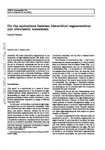
Fig. 2. An example of the real (top) and imaginary (bottom) parts of . The Definition 3.12. For convenience, we have put notations indicate the widths of the constituent line elements.

from an-

original treatment of this construction ([18]) we here place it into the Riesz basis selection framework. These results are then exploited in the next section to establish a connection with a constrained binary optimization problem. Definition 3.12: Let be piecewise constant, complex functions in which are periodic and scale-ordered (as in Definition 3.2), such that, for

with

Then which hence gives ; that is, 24 uniformly spaced quantization levels are required to represent the function up to a constant. Example 3.11: For the constructions and in Example 3.7. We have . Now

which yields

. Hence

and

. Likewise,

with . Then the uniform step basis (or uniform construction) is defined by

and

whence we have , and . On the other hand, the cardinality of the (non-zero values of the) codomains of are, respectively 4 and 8. That it should take 46 quantization levels to represent only 8 different values motivates the construction in Section III.C where the dynamic range is equal to the codomain cardinality (cf. power-of-two filters [14]). In other words, the dynamic range is optimal; constraints on the dynamic range are therefore equivalent to constraints on the cardinality of the codomain. C. Uniform Construction We modify the form in (2) and, for each , put . We drop the assumption that and find an alternative to the design described by Proposition 3.5. Unlike the

An example of the construction elements are plotted in Fig. 2. Remark 3.13: Note that, akin to the exponential basis , the real and imaginary parts of the construction are designed to be even and odd, respectively. Theorem 3.14: Let be the uniform construction and let . Then, for some ,

Proof: Define the double-indexed set of intervals

NELSON: ON THE EQUIVALENCE BETWEEN A MINIMAL CODOMAIN CARDINALITY RIESZ BASIS CONSTRUCTION

Denote

the

indicator, or , namely

characteristic,

function

by

5275

is (9) with

, and

For then the construction elements can be written (5) where the normalization factor . We have

denotes the and

, is introduced to ensure

(6) Now, note that and hence that

and we have

Note that

and, in general, , where tensor, or Kronecker, product, and where

. Hence, defining , gives

(7) . which is of the specified form with Remark 3.15: We note that (7) is similar to (4) and that, once again, we require , for some ; i.e., cf. (6), we want to choose the lengths such that (8) and . for all In [18], it was shown that a solution to can be found analytically, in terms of the Sylvester-type Hadamard matrix. Theorem 3.16: (cf. [18]) Let be the th prime and let . Then a solution to

(10) are the set of odd ascending primes and and where . Proof: See [18]. Remark 3.17: Note that the Hadamard-Sylvester solution (9) not only ensures that all terms in the sum of (7), or equivalently in (8), are cancelled for but that they are also cancelled for all multiples of . Example 3.18: 1) Setting , gives and (7) and (8) are zero for . 2) Setting , gives and (7) and (8) are zero for . 3) Setting , gives and (7) and (8) are zero for . Note that but we wanted . However, cf. Fig. 2 and note that, from Definition 3.2, the are -periodic; hence, adding a construction element with width 53/210 is equivalent to adding a width of 52/210 (the overlapping segments cancel). 4) Setting , gives and (7) and (8) are zero for . Note that but we wanted . However, again noting 2 and Definition 3.2, adding a construction element with width 68/210 is equivalent to adding a width of 37/210 (the overlapping segments cancel). IV. MINIMUM CARDINALITY FRAMEWORK The previous section described a zero-degree basis construction with small dynamic range. In this section Corollary 4.1 below confirms that this is also a solution to an instance of the optimization problem stated in Definition 2.2. A. Relationship Between the Minimum Cardinality Cost Function and the Hadamard-Sylvester Solutions Recall that the goal is to approximate elements of the orthonormal basis, over a local subset of their ‘analysis domain’ (e.g., over a local subset of Fourier coefficients) with superpositions of piecewise polynomial Riesz basis functions, subject to cardinality constraints on the codomain.

5276

IEEE TRANSACTIONS ON SIGNAL PROCESSING, VOL. 62, NO. 20, OCTOBER 15, 2014

Now recall the objective function given by Definition 2.2. For a basis, say, that satisfies Definition 3.2, we want to minimize the cost function subject to cardinality constraints on the scaled basis codomain:

By construction, the uniform step basis has and is normalized (by the constant ) such that Hence, for the uniform construction, we want to minimize

.

Theorem 4.2: Let be the uniform construction with associated cost function . Then there exand binary vector ists a matrix such that

Proof: We note firstly that, by virtue of the Fourier series derivative property , the objective function becomes

(11) and where we recall the notation with respect to used earlier: . In other words, we construct the optimal by minimizing the objective function and then simply use property (3) of Definition 3.2 to set . Ostensibly, this can be seen as an integer valued, cardinality-constrained, filter bank version of the sparsity constrained, finite impulse response construction problem discussed by Baran et al. [3]. The previous section showed an analytical solution to a very similar cost minimization problem and we can now state this connection as follows. Corollary 4.1: Define the cost function, cf. Definition 2.2

Let and let denote the largest prime. Let be the th order Hadamard-Sylvester matrix and let be defined as in (10). Then the Hadamard-Sylvester solution also solves

Proof:

(12) where the derivatives should be interpreted in the distributional , we can sense. For small enough write (the piecewise constant function) in discretized form as the vector

i.e., the construction lengths are discretized as . For then, the operator becomes an appropriately scaled, and truncated, discrete Fourier transform matrix with elements proportional to , for and . Hence, the objective function is

with constraint where . Here, the elements in the matrix are scaled (all by the same constant factor) such that the vector takes integer values. Hence, (12) becomes

where

is the (circular) discrete difference operator with for and ;

and where

where the first equality follows from the definition of the cost function, cf. (11), the second equality results from Theorem 3.14, and the fourth equality is a consequence of the orthonormality of . We then note, from Theorem 3.16, that the Hadamard-Sylvester solution gives .

We note here that is a vector with elements in . However, by virtue of Definition 2.3, since is Hermitian (the real part is even and the imaginary part is odd) we can multiply the necessary real and imaginary parts of the coefficients in the Fourier matrix, say , and define the (circular) absolute difference operator . We then have

B. Relationship Between the Minimum Cardinality Cost Function and Constrained Binary Optimization Since the problem described in (11) involves piecewise constant functions, we can frame it as a constrained binary optimization problem, as follows.

Now, is a vector with elements in , and the minimization is a constrained optimization problem, subject to the constraint that is binary and that .

NELSON: ON THE EQUIVALENCE BETWEEN A MINIMAL CODOMAIN CARDINALITY RIESZ BASIS CONSTRUCTION

C. Relationship Between the Constrained Binary Optimization and the Hadamard-Sylvester Solutions We therefore arrive at the interesting result that the Hadamard-Sylvester solutions intersect with a subset of binary optimization solutions. Corollary 4.3: Let and let denote the largest prime. The Hadamard-Sylvester solution (cf. Theorem 3.16) solves the binary optimization problem

subject to , with and . Proof: Result follows immediately from Corollary 4.1 and Theorem 4.2. Remark 4.4: The parameter in the matrix controls the size of the subset of frequency components around (i.e., ‘base-bandwidth’) over which we compare the Riesz basis with the orthonormal basis. That these components decay as serves as motivation to minimize the distance between the bases over finite . In this sense, it is tempting to also parameterize the matrix by introducing a decay exponent to control the weight or importance of the components near to zero. We then arrive at the following generalization of the objective function, namely

5277

We can now consider the problem of constructing the piecewise polynomials to locally approximate , i.e., we generalize the cost function from (12) to the form

But, this is equivalent to raising the weighting matrix to the power of and we have that

in (13)

Hence, optimizing the construction of order piecewise polynomials is equivalent to performing a constrained binary optimization of the piecewise constant construction with a weight matrix decay of . The examples given in Fig. 3 show that, as expected, these functions approximate the orthonormal basis (of complex exponentials ) with increasing accuracy as either the number of construction elements is increased and/or as the order of the polynomial is increased. B. Convolution Family Definition 5.3: Let be the uniform construction. Let satisfy Definition 3.2, with . Then, define

(13) Remark 5.4: Note that . Hence, the alternative way to construct piecewise polynomials to locally approximate is to minimize

V. EXTENSIONS TO HIGHER ORDER POLYNOMIALS The piecewise constant construction can be extended to piecewise polynomials in at least two ways, namely antiderivatives and convolutions. These are treated in the next two subsections below.

With weights, this is

A. Antiderivative Family Definition 5.1: Let struction given above. Let

such that by

be the uniform consatisfy Definition 3.2, with

and where the constant

ensures that Remark 5.2: Note that antiderivatives of :

. , over , is the family of

, defined

th

Hence, optimizing this alternative construction of order piecewise polynomials is equivalent to performing a constrained binary optimization of the piecewise constant construction with respect to an , rather than an , norm. Similar to Fig. 3, the examples given in Fig. 4 show that these extensions approximate the orthonormal basis with increasing accuracy as either the number of construction elements is increased and/or as the order of the polynomial is increased. VI. EXPERIMENTS

Furthermore, we have that

Corollary 4.3 gives the result that the Hadamard-Sylvester (analytical) solution coincides with the solution to the Fourier basis version of the binary optimization problem for . In addition to the proofs given in the previous

5278

IEEE TRANSACTIONS ON SIGNAL PROCESSING, VOL. 62, NO. 20, OCTOBER 15, 2014

Fig. 3. Antiderivative extension to order and polynomials. As either the number of ‘levels’ , or the order is increased, the functions become more sinusoidal.

Fig. 4. Convolution extension to order and polynomials. As either the number of ‘levels’ , or the order is increased, the functions become more sinusoidal.

section, this is now corroborated experimentally. Of added interest, here, is to investigate the numerical solutions for the case . That is, whether a numerical solution can cancel out more harmonics than the Hadamard-Sylvester solution or whether the analytical solution is as good as it gets in this regard. Tables I, II, III show the numerically optimized values of the length parameter for respectively. These are computed, via an exhaustive search, with , for several weight decays , and for several bandwidths . The is chosen in this way to ensure that the search intervals are discretized sufficiently finely that they contain the exact Hadamard-Sylvester solutions given by Theorem (3.16). Figs. 5, 6, 7 illustrate the ‘optimal’ basis functions (in the sense of (13)) found by the numerical minimization for a selection of different decays and bandwidths. In particular, the tables show that the Hadamard solution given by (9) is found by the minimizer for:

. This confirms our previous analytic findings that we can zero out: the 3rd harmonic of ; the 3rd and 5th of ; and the 3rd, 5th, and 7th harmonics of . The numerical results also show that we cannot do better than the analytic solution; that is, for , we cannot zero out both the 3rd and 5th harmonic; or, for we cannot zero out the 3rd, 5th, and 7th harmonic. We can also see that analytic solution prevails in some cases where the bandwidth is increased (the Hadamard solution appears in more than one row and column in the tables). Furthermore, this holds for solution more than it does for the solution. This reflects two things: (1) the harmonics of the construction elements decay as so that the lower harmonics contain most of the ‘error’; (2) minimization tends to lead to solutions which spread the error over several series coefficients whereas the solution, is better at inducing ‘sparsity’ in the series coefficients. On the other hand, increasing the

NELSON: ON THE EQUIVALENCE BETWEEN A MINIMAL CODOMAIN CARDINALITY RIESZ BASIS CONSTRUCTION

TABLE I FOR VARIOUS WEIGHT DECAYS AND OPTIMAL LENGTH PARAMETERS BANDWIDTHS FOR THE CASE. THE TOP FOUR ROWS ARE THE SOLUTIONS; THE BOTTOM FOUR ARE THE SOLUTIONS. (THE ENTRIES BELOW ARE ALL FRACTIONS OF 420; NOTE, FROM EXAMPLE 3.18, PART 1, THE HADAMARD SOLUTION: )

5279

TABLE III FOR VARIOUS WEIGHT DECAYS AND OPTIMAL LENGTH PARAMETERS BANDWIDTHS FOR THE CASE. THE TOP FOUR ROWS ARE THE SOLUTIONS; THE BOTTOM FOUR ARE THE SOLUTIONS. (THE ENTRIES BELOW ARE ALL FRACTIONS OF 420; NOTE, FROM EXAMPLE 3.18, PARTS 3 AND 4, THE HADAMARD SOLUTIONS: AND )

TABLE II FOR VARIOUS WEIGHT DECAYS AND OPTIMAL LENGTH PARAMETERS BANDWIDTHS FOR THE CASE. THE TOP FOUR ROWS ARE THE SOLUTIONS; THE BOTTOM FOUR ARE THE SOLUTIONS. (THE ENTRIES BELOW ARE ALL FRACTIONS OF 420; NOTE, FROM EXAMPLE 3.18, PART 2, THE HADAMARD SOLUTION: )

weight decay can also help the minimizer find the Hadamard solution for lower order constructions; this is because the decay penalizes the lower harmonics more than the higher harmonics. In Fig. 5, a selection of ‘optimal’ uniform constructions are plotted (on the interval ), alongside (for illustrative purposes) the Fourier series coefficients of their derivative. (Note, that the Fourier series of the non-differentiated function is simply multiplied by the series of the derivative.) The first column shows the optimal solution for , i.e., over the Fourier coefficients ; this particular case coincides with the Hadamard solution given by Example 3.18, part 1, (which gives a minimum cost function of zero) whereas the norm solution does not. The solution induces sparsity in the coefficient at the cost of a relatively larger error in the coefficient. In this sense, the solution obtains a better ‘local’ approximation to . In the second column, we see that, by widening the ‘bandwidth’ to , neither norms produce the same minimum as the Hadamard solution. It is clear that a zero minimum does not exist in this case. Furthermore, from the Fourier series plot, we can see that the solution spreads the error between , and 7; whereas, the solution zeros out the Fourier coefficient at and spreads the error between and 7. The sparsity inducing effect of increasing the weight decay can be seen in the third column. In this case, the Hadamard solution is obtained (exactly for and approximately for ) over coefficients .

Figs. 6 and 7 also show the optimal solutions (in the sense that they remove the 3rd and 5th or 3rd, 5th, and 7th harmonics respectively) found by both norms in the first column and other solutions in the second and third column. Interestingly, the first column of Fig. 7 shows that the and norms find two different Hadamard solutions; finds Example 3.18, part 3 and finds Example 3.18, part 4. Indeed, the solution might be deemed marginally better; the basis function contains more zeros and the first non-zero Fourier series coefficient at is smaller than that of the solution. (Regrettably, we cannot offer a satisfactory explanation for this.) VII. CONCLUSION AND FURTHER WORK The work presented above shows how minimal cardinality Riesz basis approximations to orthogonal bases can be constructed by inducing sparsity in the distributional derivatives. We have shown that this is equivalent to a constrained binary optimization problem and, for the case of the Fourier series basis, we have found that the solutions intersect those found with Sylvester-type Hadamard matrices [18]. However, following a remark made in Section IV, the first column of Fig. 7 poses the question of whether it is possible to prove which Hadarmard solution corresponds to the solution and which one corresponds to the solution? Furthermore, since both solutions are optimal, how do we choose between them? Other possible further work is briefly outlined, as follows. The discussed framework affords the possibility of generalizing the sparse filter construction of Baran et al. [3] to the filter-bank, integer valued case. For example, if we require a low-cardinality approximation to a Riesz basis over some indexing subset , then the cost function in Definition 2.2 becomes: . The construction elements would, of course, have to be modified from (5), depending on what kind of Hilbert space the are defined in. A particular challenge would be whether an analytical solution exists (cf. the Hadamard solution for the uniform construction) and how it would be found. As an aside, reinterpreting

5280

IEEE TRANSACTIONS ON SIGNAL PROCESSING, VOL. 62, NO. 20, OCTOBER 15, 2014

Fig. 5. Uniform constructions for and a selection of ‘bandwidths’, in the first row and the Fourier series of the derivative in the second row.

, and weight decays . The (imaginary part of the) ‘time-domain’ function is shown

Fig. 6. Uniform constructions for and a selection of ‘bandwidths’, in the first row and the Fourier series of the derivative in the second row.

, and weight decays . The (imaginary part of the) ‘time-domain’ function is shown

Fig. 7. Uniform constructions for and a selection of ‘bandwidths’, in the first row and the Fourier series of the derivative in the second row.

, and weight decays . The (imaginary part of the) ‘time-domain’ function is shown

the Hilbert space as a Paley-Wiener space gives rise to a simple instance of the compressive sensing type problem, namely that of minimizing a cost over the discrete sampled time domain, subject to sparsity constraints in the frequency domain. Motivated by the approximate signal processing philosophy of Nawab and Dorken [16], an iterative refinement algorithm was proposed in [18]. This decomposed the uniform, piecewise constant construction such that the resulting transform could be performed iteratively. However, this scheme was purely deterministic. Instead, since the error will depend on the complexity

of the signal, it would be of interest to explore a probabilistic approach, cf. Winograd and Nawab [28], to predict the signal dependent algorithmic complexity in an adaptive manner. The Mobius construction plays a central part of both the wavelet filter enhancement scheme of [19] and the multichannel, multisampling rate theorem of [17]. It is tempting, therefore, to explore a development of these ideas using, instead, the uniform construction. Iserles and Nørsett [11] introduce a modification to the Fourier transform (a shift in the imaginary part of the basis

NELSON: ON THE EQUIVALENCE BETWEEN A MINIMAL CODOMAIN CARDINALITY RIESZ BASIS CONSTRUCTION

functions) which induces a stronger decay in the Fourier series. Very much in contrast, the work presented here focuses on the behavior of our modified transform over the coefficients for rather than the decay as . Notwithstanding, it should be possible to combine both of these ideas and explore the idea of introducing a shift in the imaginary part of the uniform, piecewise constant basis. As Iserles and Nørsett show, however, that justifying this seemingly simple shift with sufficient rigor requires much care and is also, therefore, left as further work. ACKNOWLEDGMENT The author is most grateful for the reviewers’ detailed comments and suggestions. In addition, the author would like to extend special thanks to Kelly Watson–Nelson for her comments and kind support throughout the preparation of this paper.

REFERENCES [1] D. Anastasia and Y. Andreopoulos, “Software designs of image processing tasks with incremental refinement of computation,” IEEE Trans. Imag Process., vol. 19, no. 8, pp. 2099–2114, 2010. [2] T. M. Apostol, Introduction to Analytic Number Theory. New York, NY, USA: Springer, 1976. [3] T. Baran, D. Wei, and A. V. Oppenheim, “Linear programming algorithms for sparse filter design,” IEEE Trans. Signal Process., vol. 58, no. 3, pp. 1605–1617, 2010. [4] E. J. Candès, “New ties between computational harmonic analysis and approximation theory. approximation,” Innovations Appl. Math., pp. 87–153, 2002. [5] E. J. Candès, Y. Eldar, D. Needell, and P. Randall, “Compressed sensing with coherent and redundant dictionaries,” J. Appl. Comput. Harmon. Anal., vol. 31, pp. 59–73, 2010. [6] S. S. Chen, D. L. Donoho, and M. A. Saunders, “Atomic decomposition by basis pursuit,” SIAM J. Scientif. Comput., vol. 20, pp. 33–61, 1998. [7] M. Gaster and J. B. Roberts, “On the spectral analysis of randomly sampled records by a direct transform,” Proc. Roy. Soc. A, vol. 354, pp. 27–58, 1977. [8] T. I. Haweel and A. Alhasan, “A simplified square wave transform for signal processing,” in An International Conference on Mathematical Analysis and Signal Processing, ser. Contemporary Mathematical Series. Providence, RI, USA: Amer. Math. Soc., 1994, pp. 265–271. [9] H. Hedenmalm, P. Lindqvist, and K. Seip, “A Hilbert space of Dirichlet ,” Duke Math. J., vol. series and systems of dilated functions in 86, pp. 1–37, 1997. [10] R. D. Hughes and M. L. Heron, “Approximate Fourier transform using square waves,” Proc. Inst. Electr. Eng —A, vol. 136, pp. 223–228, 1989. [11] A. Iserles and S. P. Nørsett, “From high oscillation to rapid approximation I: Modified fourier expansions,” IMA J. Numer. Anal., vol. 28, pp. 862–887, 2008. [12] N. G. Kingsbury, “Complex wavelets for shift invariant analysis and filtering of signals,” J. Appl. Comput. Harmon. Anal., vol. 10, no. 3, pp. 234–253, 2001.

5281

[13] M. P. Lamoureux, “The Poorman’s transform: Approximating the Fourier transform without multiplication,” IEEE Trans. Signal Process., vol. 41, no. 3, pp. 1413–1415, 1993. [14] D. Li, Y. C. Lim, Y. Lian, and J. Song, “A polynomial-time algorithm for designing FIR filters with power-of-two coefficients,” IEEE Trans. Signal Process., vol. 50, no. 8, pp. 1935–1941, 2002. [15] V. Lohweg, C. Diederichs, and D. Müller, “Algorithms for hardwarebased pattern recognition,” EURASIP J. Appl. Signal Process., vol. 12, pp. 1912–1920, 2004. [16] S. Nawab and E. Dorken, “Efficient STFT approximation using a quantization and differencing method,” in Proc. IEEE Int. Conf. Acoust., Speech, Signal Process., 1993, vol. 3, pp. 587–590. [17] J. D. B. Nelson, “A multi-channel, multi-sampling rate theorem,” Sampl. Theory Signal Image Process.: An Int. J., vol. 2, pp. 83–96, 2003. [18] J. D. B. Nelson, “On the coefficient quantization of the Fourier basis,” IEEE Trans. Signal Process., vol. 51, no. 7, pp. 1838–1846, 2003. [19] J. D. B. Nelson, “A wavelet filter enhancement scheme with a fast integral B-wavelet transform and pyramidal multi-B-wavelet algorithm,” J. Appl. Comput. Harmon. Anal., vol. 18, pp. 234–251, 2005. [20] J. Pender and D. Covey, “New square wave transform for digital signal processing,” IEEE Trans. Signal Process., vol. 40, no. 8, pp. 2095–2097, 1992. [21] J. E. T. Penny, M. I. Friswell, and D. J. Inman, “Approximate frequency analysis in structural dynamics,” Mechan. Syst. Signal Process., vol. 27, pp. 370–378, 2012. [22] I. W. Selesnick, R. G. Baraniuk, and N. G. Kingsbury, “The dual-tree complex wavelet transform,” IEEE Signal Process. Mag., vol. 22, no. 6, pp. 123–151, 2005. [23] W. Sweldens, “The lifting scheme: A custom-design construction of biorthogonal wavelets,” J. Appl. Comput. Harmon. Anal., vol. 3, no. 2, pp. 186–200, 1996. [24] D. W. Tufts and G. Sadasiv, “The arithmetic Fourier transform,” IEEE ASSP Mag., vol. 5, pp. 13–17, 1988. [25] W. J. Walker, “Sampling theory and the Arithmetic Fourier Transform,” in Sampling Theory in Fourier and Signal Analysis: Advanced Topics, J. R. Higgins and R. L. Stens, Eds. New York, NY, USA: Oxford Univ. Press, 1999, ch. 2, pp. 38–55. [26] Y. Wei, “Dirichlet multiplication and easily-generated function analysis,” Comput. Math. Appl., vol. 39, pp. 173–199, 2000. [27] Y. Wei, “Frequency analysis based on easily generated functions,” J. Appl. Comput. Harmon. Anal., vol. 8, pp. 280–285, 2000. [28] J. Winograd and S. H. Nawab, “Probabilistic complexity analysis for a class of approximate DFT algorithm,” J. VLSI Signal Process., vol. 14, pp. 193–205, 1996. [29] A. Wintner, An Arithmetical Approach to Ordinary Fourier Series. Baltimore, MD, USA: Waverly Press, 1945. James D. B. Nelson joined the Department of Statistical Science at University College London as a Lecturer (Assistant Professor) in 2010 and became Senior Lecturer (Associate Professor) in 2013. After a Ph.D. in applied harmonic analysis from the Mathematics Department at Anglia Polytechnic University (1998–2001), he held post-doc positions in: the Applied Mathematics and Computing Group at the University of Cranfield (2001–2004); the Information: Signals, Images, and Systems Research Group at the University of Southampton (2004–2006); and the Signal Processing and Communications Laboratory at the University of Cambridge (2006–2010). Dr. Nelson’s interests span aspects of harmonic analysis, signal processing, computational statistics, and machine learning.