On the equivalence between complementarity systems, projected ...

Systems & Control Letters 55 (2006) 45 – 51 www.elsevier.com/locate/sysconle

On the equivalence between complementarity systems, projected systems and differential inclusions! B. Brogliatoa,∗ , A. Daniilidisb , C. Lemaréchala , V. Acarya a INRIA, Bipop Research Team, 655 avenue de l’Europe, Montbonnot, 38334 Saint Ismier, France b Departement de Matemàtiques, Universitat Autònoma de Barcelona, 08193 Bellaterra, Spain

Received 20 January 2004; received in revised form 22 November 2004; accepted 8 May 2005 Available online 22 June 2005

Abstract In this note, we prove the equivalence, under appropriate conditions, between several dynamical formalisms: projected dynamical systems, two types of differential inclusions, and a class of complementarity dynamical systems. Each of these dynamical systems can also be considered as a hybrid dynamical system. This work both generalizes previous results and sheds some new light on the relationship between known formalisms; besides, it exclusively uses tools from convex analysis. © 2005 Elsevier B.V. All rights reserved. Keywords: Complementarity systems; Projected dynamics; Unilateral dynamics; Hybrid dynamical systems; Differential inclusions

1. Introduction, notation Unilateral dynamical systems have long been studied in the applied mathematics literature [18,19,3,13,20], because they find important applications in various fields (like mechanics, economics, and electrical circuits as shown recently in [5]). They usually take the form of differential inclusions or variational inequalities. In parallel, the theory of complementarity problems has witnessed an impressive development [8,10], essentially motivated by optimization problems. Recently, complementarity systems, which consist of ordinary differential equations coupled to complementarity conditions, have been the object of in depth studies in the control literature [11,4]. Basic convex analysis tells us that complementarity problems can equivalently be formulated as a special type of generalized equations (i.e. equations of ! This work was partially supported by the European project SICONOS IST 2001-37172. ∗ Corresponding author. Tel.: +33 4 76615393; fax: +33 4 76615477. E-mail addresses: [email protected] (B. Brogliato), [email protected], [email protected] (A. Daniilidis), [email protected] (C. Lemaréchal), [email protected] (V. Acary).

0167-6911/$ - see front matter © 2005 Elsevier B.V. All rights reserved. doi:10.1016/j.sysconle.2005.04.015

the form 0 ∈ F (x), where F (x) is multivalued). This suggests that there should also exist close links between complementarity systems and unilateral dynamical systems. From a general perspective in the study of hybrid dynamical systems and their control, it seems quite important to clarify the relationships between these various formalisms. First steps in this direction can be found in [12,4]. Thus, the object of this note is to study the relationship between a number of conspicuously different formalisms: projected dynamical systems [22, Section 2.2], two types of differential inclusions [3], and complementarity dynamical systems [11,4]. We will also discuss the existence of solutions to these systems. For other works related to these problems, see [13,7,24]. Our material is fairly standard, concerning convex analysis (for example [14], mainly its Chapter III) and differential inclusions [3]. We work with Rn considered as a Euclidean space, with scalar product #x, y$ and associated norm %x%. Recall that the normal cone to a nonempty closed convex set K ⊂ Rn at x ∈ K is NK (x) := {s ∈ Rn : #s, y − x$!0, for all y ∈ K},

46

B. Brogliato et al. / Systems & Control Letters 55 (2006) 45 – 51

while the tangent cone is the polar of the normal cone, which means TK (x) := [NK (x)]◦ := {d ∈ Rn : #s, d$ !0,

for all s ∈ NK (x)}

(if x ∈ / K, we set NK (x) = TK (x) = ∅). In this paper we are given a nonempty closed convex set C ⊂ Rn (the feasible set) and two measurable functions g : R+ → Rn and f : Rn → Rn . Associated with the data, we consider (together with the initial condition x(0) = x0 ∈ C) • the Projected Dynamical System

a.e. x(t) ˙ = projTC (x(t)) (−f (x(t)) − g(t))

(PDS)

• and the two Differential Inclusions (the first one being implicit) a.e. −x(t) ˙ ∈ f (x(t))+g(t)+NTC (x(t)) (x(t)), ˙ a.e. −x(t) ˙ ∈ f (x(t)) + g(t) + NC (x(t)),

(UDI-TC ) (UDI-C)

the notation UDI stresses the fact that the right-hand side is an unbounded set (while differential inclusions are often stated with a compact right-hand side). A solution to any of the above relations is understood as an absolutely continuous function t + → x(t); a.e. means almost everywhere with respect to t, in the Lebesgue measure. Note that any solution to any of the above systems must by necessity lie in C for almost every t. Remark 1. By the definition of the normal cone, (UDI-C) can also be formulated as a variational inequality: a.e. x(t) ∈ C

and

a.e. #x(t) ˙ + f (x(t)) + g(t), y − x(t)$ " 0 for all y ∈ C. The analogous transformation for (UDI-TC ) is more sophisticated as the set in the right-hand side also depends on x(t): ˙ we obtain a.e. (x(t), x(t)) ˙ ∈ C × TC (x(t)) and a.e. #x(t) ˙ + f (x(t)) + g(t), y − x(t)$ ˙ " 0 for all y ∈ TC (x(t)), a sort of quasi-variational inequality. This remark is important, as (quasi-)variational inequalities form a widely studied subject; see for example [15,2,21,10]. In [9,22,12], (PDS) is presented under two ostensibly different—but in fact equivalent—formulations, see (2) and (4) below. The equivalence between (2) and (4) has been established in [12, Theorem 5.1 and Remark 5.3]. For the reader’s convenience, in Section 2.1 we give straightforward

arguments to establish directly the equivalence of each of these two formulations with (PDS). The first contribution of this paper is to clarify the equivalence between the formulations (PDS) (or equivalently, (2) or (4)), (UDI-TC ) and (UDI-C). More precisely, Corollary 2 will state that (PDS) and (UDI-TC ) are always equivalent, while (UDI-C) may have more solutions. Full equivalence holds when (UDI-C) has (no solution at all or) a unique solution which is slow, i.e. x(t) ˙ is of minimal norm in the set it belongs to:1 − x(t) ˙ = f (x(t)) + g(t) + !¯ (t), with !¯ (t) = argmin %f (x(t)) + g(t) + !%. !∈NC (x(t))

The above considerations are purely geometric and concern an abstract feasible set C. In practice, however, C is often explicitly described by constraints: C = {x ∈ Rn : h(x) !0 ∈ Rm },

(1)

where h(·) := (h1 (·), . . . , hm (·))- and the functions hi : Rn → R, i = 1, . . . , m are hereby assumed to be continuously differentiable. The gradient of hi at x is ∇hi (x) ∈ Rn , so that the first-order approximation of hi close to x is written as hi (x + d) = hi (x) + #∇hi (x), d$ + o(%d%) for all d ∈ Rn . The constraint-space Rm is equipped with the standard ! dot-product: we! write "- h for m i=1 "i hi and the notation n ∇h(x)" means m i=1 "i ∇hi (x) ∈ R . The nonnegative orm thant of R is m Rm + := {" ∈ R : "i "0, i = 1, . . . , m}.

We will also use the notation " "0 when " ∈ Rm + , likewise for the nonpositive orthant Rm . − With the above notation, in addition to (PDS) and (UDI) we consider: • the Complementarity Dynamic System a.e. − x(t) ˙ = f (x(t)) + g(t) + ∇h(x(t))"(t),

a.e. a.e. 0 " h(x(t)) ⊥ "(t) " 0,

(CDS)

(⊥ means orthogonality: "- h = 0, and "(·) is assumed to be measurable). The second contribution of this paper is to relate the above formalism to the ones previously mentioned; this is done in Proposition 3. The pivot is (UDI-C): it may have more 1 Being closed and convex, this set has a unique point of minimum norm. The measurability of the solution x(t) ensures the measurability of the multifunction NC (x(t)), and thus of its minimal selection !(t) (see [6] for more details).

47

B. Brogliato et al. / Systems & Control Letters 55 (2006) 45 – 51

solutions than (CDS); however, equivalence holds if some additional constraint qualification holds. The above-mentioned results are intrinsic, and thus independent of any existence question. When existence does hold, these results can be made more accurate. For this, the pivot is again (UDI-C): under an appropriate assumption of monotonicity type, it has a unique solution, which is slow (see Theorem 1). In view of the above results, the same property therefore holds for the other formulations. In [12, Section 4], the equivalence between the formalisms of Section 2.1 and (CDS) is stated under assumptions guaranteeing likewise existence and uniqueness. An important difference from the present paper is that we exclusively use general tools from convex analysis, which turn out to substantially clarify the role of the respective assumptions (revealing in particular the crucial role of slowness).

Proof. By the definition of N ◦ , there exists at least one ! in (3a) such that #!, v$ > 0; hence, the optimal value is positive and must be attained at some !∗ of norm 1. Strict convexity properties of the unit ball imply that this !∗ must be unique. The first statement is proved. Now the projection of v onto N is the unique solution of min %! − v%2 , !∈N

or equivalently min{%! − v%2 : %!% =% projN (v)%} !∈N

(the extra constraint being redundant!). Up to the constant %v%2 + %projN (v)%2 , the above optimization problem is equivalent to min{−#!, v$, %!% =% projN (v)%}. !∈N

2. Basic equivalences We start by establishing some equivalences which do not use the fact that x(t) ˙ is the (time) derivative of x(t). In fact, x(t) and x(t) ˙ are considered as two independent vectors of Rn .

In view of positive homogeneity, this latter problem has a unique solution colinear to that of (3b), namely %projN (v)%!∗ . The proof is complete. # Note that projN (v) = 0 if v ∈ N ◦ . Take x ∈ C and N := NC (x); then, we see from (3a) that the operator $C used in [22] and [12, Section 2] is equal to $C (x, v) = v − #!∗ , v$!∗ ,

2.1. Equivalent formulations of (PDS) In [9], [22, Definition 2.5] and [12, Definition 2.1], (PDS) is defined under different forms. The first one is2

where !∗ is given in Lemma 1. For the following result, see also [12, Remark 5.3].

projC (x(t) + #v) − x(t) a.e. x(t) ˙ = lim , # #↓0

Corollary 1. Set v := −f (x(t))−g(t) and N := NC (x(t)). Use the notation of Lemma 1, setting !∗ = 0 if v ∈ N ◦ = TC (x(t)). Then, the right-hand side of (PDS) is

(2)

where x(t) ∈ C and v := −f (x(t)) − g(t). The following result directly links (2) to (PDS).

projTC (x(t)) (v) = v − projN (v) = v − #!∗ , v$!∗ .

Proposition 1. The right-hand sides of (PDS) and (2) are the same. Proof. This is Proposition III.5.3.5 of [14].

#

Another form of (PDS) is presented in [22,12], for which we need special notation: !∗ introduced in the next elementary lemma, and $C after it. / N ◦, Lemma 1. Given a closed convex cone N ⊂ Rn and v ∈ the optimization problems max{#!, v$ : ! ∈ N, %!%!1},

(3a)

max{#!, v$ : ! ∈ N, %!% = 1}

(3b)

have the same value % > 0 and the same unique solution !∗ . projN (v) Besides, projN (v) 1 = 0 and !∗ = . %projN (v)%

2 The notation # → 0 of [9,22,12] assumes # > 0, i.e. # ↓ 0. In fact, the difference quotient in (2) need not have a limit when # is allowed to take on either sign.

Proof. Since TC (x(t))=[NC (x(t))]◦ , Moreau’s decomposition theorem3 states that the right-hand side of (PDS) is v − projN (v). Then use Lemma 1, recalling that #projN (v), v$ = %projN (v)%2 . # This gives an alternative proof of the equivalence of (PDS) with the other formulation of [22,12], namely x(t) ˙ = $C (x(t), −f (x(t)) − g(t)).

(4)

2.2. Geometric formulations: Relations between (PDS) and (UDI) In this subsection, we deal with the case of an abstract set C, not necessarily described by constraints. 3 See [14, Theorem III.3.2.5]: two mutually polar cones N and N ◦ decompose the space. More precisely, the projections onto N and N ◦ of a given v ∈ Rn are the unique elements in N and N ◦ , respectively, mutually orthogonal, and summing up to v:

v = projN (v) + projN ◦ (v),

#projN (v), projN ◦ (v)$ = 0.

48

B. Brogliato et al. / Systems & Control Letters 55 (2006) 45 – 51

(ii) (UDI-TC ) holds, and (iii) (UDI-C) holds, together with the following two equivalent properties:

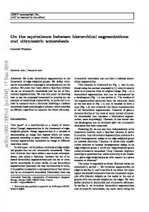
υ = -f(x) - g K = TC(x)

s

υ−s

(iii)1 −x(t)=f ˙ (x(t))+g(t)+projNC (x(t)) (−f (x(t))− g(t)), and (iii)2 the vector −x(t) ˙ is of minimum norm in f (x(t)) + g(t) + NC (x(t)).

C x K° = NC(x)

Fig. 1. The only possible solution to (PDS) and (UDI-TC ).

Proposition 2. Let K ⊂ Rn be a nonempty closed convex cone. For any two vectors v and s in Rn , the following relations are equivalent: s = projK (v),

(5a)

v − s ∈ NK (s),

(5b)

s ∈ K,

◦

v−s ∈K , ◦

v−s ∈K ,

◦

∀! ∈ K ,

#v − s, s$ = 0, 2

%s% !#s, v − !$.

(5c) (5d)

Proof. Use the variational characterization of a projection: (5a) is equivalent to s∈K

and #v − s, s 3 − s$!0, for all s 3 ∈ K.

(6)

By the definition of a normal cone, this is exactly (5b). Since K is a cone, NK (s) = K ◦ ∩ s ⊥ (here s ⊥ denotes the subspace orthogonal to s); it follows that (5b) is also equivalent to (5c). Now let v and s satisfy (5c) and take ! ∈ K ◦ ; because s ∈ K, we have #!, s$!0 = #v − s, s$;

hence, %s%2 !#v, s$ − #!, s$

and (5d) holds. Conversely, let v and s satisfy (5d). In particular, #!, s$ is bounded from above (by #s, v$ − %s%2 ) when ! describes the cone K ◦ , and therefore cannot be strictly positive;4 thus, #!, s$!0 for all ! ∈ K ◦ , i.e. s ∈ K ◦◦ = K; combining v − s ∈ K ◦ with s ∈ K, we have #s, v − s$!0. Besides, take ! = 0 in (5d) to see that #s, s − v$ !0. Piecing together, (5c) holds and the proof is complete. # The form (5c) clearly reveals that s and v − s make up the Moreau decomposition of s + v − s = v; in particular, it follows that v − s = projK ◦ (v). Thus, the mere relation (5b) implies that both s and v − s are fairly special points in their respective cones. This is illustrated by Fig. 1 (where t is dropped), and the link with Problems (PDS) and (UDI) of Section 1 is clear: Corollary 2. Given two vectors x =x(t) ∈ C and x˙ = x(t) ˙ ∈ Rn , the following three statements are equivalent:

Proof. Apply Proposition 2 with K := TC (x(t)) (which is nonempty), and v := −f (x(t)) − g(t), s := x(t); ˙ note that K ◦ = NC (x(t)). Then (5a) = (PDS), (5b) is (UDI-TC ) and the first line of (5d) is (UDI-C). Now write the second line in (5d) as #0 − (−s), (! − v) − (−s)$!0 for all (! − v) ∈ K ◦ − v to see that it means −s = projK ◦ −v (0): −s = argmin %!%, !∈K ◦ −v

which is (iii)1 . The form (iii)2 appears with the change of variable ! + v = !3 : −s = argmin %!3 − v%. # !3 ∈K ◦

Thus, (UDI-C) is equivalent to the other ones if and only if it has the so-called slow solution [7] (that is, x(t) ˙ is of minimal norm) as the only possible solution. Note also that the last form in the statement of Corollary 2 can be written as x(t)=v ˙ −projNC (x(t)) (v) with v =−f (x(t))−g(t), which is just the formulation of [22,12] (recall Corollary 1). An important consequence of the above results is that (UDI-TC ) is the equivalent form of (PDS), in terms of differential inclusions. 2.3. Formulation using constraints explicitly In this subsection, we turn to (CDS), which requires some more notation and material from convex analysis. For x ∈ C, we denote by I (x) := {i ∈ {1, . . . , m} : hi (x) = 0}

(7)

the set of active constraints at x and we linearize the constraints, introducing the cones T h (x) := {d ∈ Rn : #∇hi (x), d$ !0, i ∈ I (x)}, h ◦ N h (x) := [T  (x)]  %  = "i ∇hi (x) : "i "0, i ∈ I (x)  

(8)

i∈I (x)

(i) (PDS) holds, 4 If #! , s$ > 0 for some ! ∈ K ◦ , just take ! = t ! with t → +∞. 0 0 0

(still with the convention T h (x) = N h (x) = ∅ if x ∈ / C). Note that they need not coincide with the usual tangent and normal

B. Brogliato et al. / Systems & Control Letters 55 (2006) 45 – 51

cones5 to C at x. Nevertheless, we always have NC (x) ⊃ N h (x) and TC (x) ⊂ T h (x). Actually, a key assumption for what follows is TC = T h , or equivalently NC =N h . This is guaranteed under any of the following qualification conditions (see [14, Section VII.2.2] for example): ∀x ∈ C, ∃d ∈ Rm for i ∈ I (x),

such that #∇hi (x), d$ < 0

(QC.1)

which is dually equivalent to the so-called Mangasarian– Fromowitz assumption: ! ) "i ∇hi (x) = 0 i∈I (x) 8⇒ "i = 0, i ∈ I (x). (QC.2) with "i "0, i ∈ I (x)

Note that (QC.2) holds in particular if

the gradients of the active constraints at x are linearly independent

(QC.3)

(just remove the restriction "i "0 in (QC.2)!). When the hi ’s are convex, it can be seen that (QC.1) is equivalent to the so-called Slater assumption6 : ¯ < 0, ∃x¯ ∈ Rn : hi (x)

i = 1, . . . , m.

(QC.4)

Proposition 3. Two vectors x = x(t) and x˙ = x(t) ˙ in Rn satisfy (CDS) if and only if they satisfy −x(t) ˙ ∈ f (x(t)) + g(t) + N h (x(t)).

(UDI-h)

If TC =T h , which holds for example under one of the qualification conditions (QC.1–4), this system is in turn equivalent to (UDI-C). Proof. Since an x(t) ∈ / C can satisfy neither system, we may assume x(t) ∈ C. The second line in (CDS) means: "i "0, i = 1, . . . , m and "i = 0 if hi (x(t)) < 0, i.e. if i ∈ / I (x). From definition (8) of N h , (CDS) is therefore exactly (UDI-h). The result follows. # Let us summarize this section: the following relations hold – S(P) standing for the solution set of a problem (P): S(PDS) = S(UDI-TC ) ⊂ S(UDI-C) ⊃ S(UDI-h) = S(CDS) and the second inclusion becomes an equality if qualification holds. The first inclusion becomes an equality when S(UDI-C) is either empty or reduces to a slow solution. As already mentioned, all of these results are static: they make no reference to t, which could be dropped from the notation. The four problems we consider could just be stated 5 With m = 1, the set C of (1) defined by the constraint h(x) := %x%2 serves as a counterexample: C ={0} but T h (0)=Rn , although TC (0)={0}. 6 The "’s describing elements of N h (x) are clearly unique when (QC.3) holds, and they form a bounded set when (QC.1)=(QC.2)=(QC.4) holds.

49

as: given f : Rn → Rn and g ∈ Rn , find x ∈ C, s ∈ Rn and " ∈ Rn such that s = projTC (x) (−f (x) − g), −s ∈ f (x) + g + NTC (x) (s),

(PS) (UI-TC )

−s ∈ f (x) + g + NC (x),

(UI-C)

s = f (x) + g + ∇h(x)", 0 "h(x) ⊥ " "0.

(CS)

The following observations are of interest when complementarity holds: (i) Generally speaking, the property v ∈ NC (x) can obviously be restated as x = projC (v + x). Hence, the above (UI-C) can also be formulated as a projection system, namely: x = projC (−s − f (x) − g + x). (ii) Likewise, we could write (UI − TC ) = (PS) in a complementarity form. In fact, (8) expresses TC (x)=T h (x) analytically via (linear) constraints. The normal cone NT h (x) (s) can therefore be computed analytically: recall from (8) that #∇hi (x), s$!0 for all i ∈ I (x) and define the set I0 (x, s) := {i ∈ I (x) : #∇hi (x), s$ = 0} of those constraints active at x ∈ C that are also active at s ∈ T h (x). Then NT h (x) (s) is the set of nonnegative combinations of the corresponding gradients: (UI-TC ) can be written as − s = f (x) + g + ∇h(x)&, #∇hi (x), s$ !0, &i "0, #∇hi (x), s$&i = 0 for i ∈ I (x). The second line above is a sort of complementarity relation, expressing that the vector & has no positive coordinate beyond I0 (x, s). However, the difficulty with a complementarity formalism is that the space where & resides depends on x: the coordinates of & are indexed in I (x). 3. Existence results The content of the previous results is void if the various systems considered in Section 1 have no solution (who would care about systems without a solution?). Existence is an even more important issue here, because of its impact on the equivalence of the various formulations. Indeed, our results in Section 2 show that the existence of a solution for (PDS) = (UDI-TC ) implies the existence of a solution for (CDS) = (UDI-C) (under constraint qualification). Conversely, the uniqueness of the solution for (CDS)=(UDI-C) implies for (PDS) = (UDI-TC ) • either non-existence,

50

B. Brogliato et al. / Systems & Control Letters 55 (2006) 45 – 51

• or uniqueness (and equivalence of all formulations) in case the solution is slow. This latter desirable situation is strongly linked to monotonicity, in the sense of [23, Chapter 12]. More precisely, we have the following result: Theorem 1. Assume that g ∈ L1 (R+ ), and that f is continuous over Rn and “hypomonotone”: there exists k "0 such that #f (x) − f (y), x − y$" − k%x − y%2 f or all x, y ∈ Rn .

(9)

Then, for any initial condition x(0) = x0 ∈ C, (UDI-C) has a unique solution x(t) over the whole of R+ , which is slow: x(t) ˙ is of minimal norm in the set f (x(t))+g(t)+NC (x(t)). Under these conditions, systems (PDS), (CDI-TC ) and (CDI-C) have the same unique solution. Furthermore, x(t) ˙ ∈ TC (x(t)). Under constraint qualification, the same holds for (CDS). Proof. The function x +→ '(x) := f (x) + kx is monotone (i.e. it satisfies (9) with k = 0). Since ' is single-valued and continuous, it is indeed maximal monotone (see [23, Example 12.7], for example). The same is true for the multivalued mapping x +−→ NC (x) ([23, Corollary 12.18] for example). Thus the multivalued mapping F := ' + NC is maximal monotone ([3, Corollary 2.7], for example). Add and subtract the term kx(t) in (UDI-C), which can be written as −x(t) ˙ ∈ F (x(t)) − kx(t) + g(t).

(UDI-C)

Applying [3, Theorem 3.17], we obtain that (UDI-C) has a unique “weak” solution—call it u(t)—on R+ satisfying u(0)=u0 ; by [3, Proposition 3.8], this solution is also strong since we are in a finite-dimensional setting. It remains to show that it is slow. Introducing the function t +→ ((t) := f (u(t)) + g(t), observe that u(t) solves the inclusion −x(t) ˙ ∈ NC (x(t)) + ((t).

(10)

But ( ∈ L1 (R+ ) and the operator NC (·) is maximal monotone; [3, Proposition 3.4] therefore guarantees that the unique solution of (10) is indeed slow: u(t) has minimum norm in the set NC (u(t)) + ((t) = f (u(t)) + NC (u(t)) + g(t). In other words, the unique solution of (UDI-C) is bound to be the slow solution. For the remaining part of the statement, it suffices to evoke Corollary 2 and Proposition 3. # Let us conclude with some remarks. (i) An interesting consequence of [3, Proposition 3.4] is the following: if g is piecewise continuous, the solution

mentioned in Theorem 1 has a right derivative x˙+ (t) at all t: “almost everywhere” can then be suppressed from the formulations, if x˙ is replaced by x˙+ . (ii) Theorem 1 is actually grounded on a fundamental result of nonlinear analysis; see [1] for example. Let F be a (multivalued) maximal monotone operator: #u − v, x − y$ "0 for all x, y and all u ∈ F (x), v ∈ F (y); then the differential inclusion x(t) ˙ + F (x(t)) : 0 has a unique solution starting at a given x(0). This solution is defined on the whole of R+ , and is slow. The refinements introduced here—see also [12]—allow a strictly positive k in (9), as well as the inhomogeneous term g(t) in the dynamics. (iii) We believe that our results easily extend to a nonconvex but so-called regular set C [23, Definition 6.4]; see also [7,25,17] for a study of differential inclusions in this context. In case of explicit constraints, C is regular when the differentiable functions hi (not necessarily convex) satisfy a qualification condition such as (QC.1)–(QC.3). (iv) A common approach to derive (UDI-TC ) from (CDS) proceeds as follows: under constraint qualification, (CDS) can be written as (see Proposition 3) − x(t) ˙ = f (x(t)) + g(t) + !, ! = ∇h(x(t))" ∈ NC (x(t)).

with

According to Proposition 2 with s = −x(t), ˙ v = −f (x(t)) − g(t) and K ◦ = NC (x(t)), this is equivalent to (UDI-TC ) = (5c) if and only if #!, x(t)$ ˙ = 0, that is, #∇h(x(t))", x(t)$ ˙ = "- w(t) ˙ = 0,

where we have set w(t) := h(x(t)) ∈ Rm (writing w˙ + (t) would be more precise). Our results clearly imply that this extra property holds if and only if the only possible solution of (UDI-C) is slow. 4. Conclusion The study of the relationships among various formalisms of hybrid systems is of interest [4], and this note sheds new light on the equivalences between complementarity systems, projected dynamical systems, and differential inclusions. In particular, (UDI-TC ) plays a prominent role: it expresses complementarity of velocities, as opposed to complementarity of positions, expressed by (UDI-C). It is commonly admitted that numerical resolution of the latter model is more difficult. An explanation could be sought in Corollary 2: when the assumptions in Theorem 1 are not satisfied (due to numerical errors, say), then (UDI-C) may have several solutions; in other words, the solution of (UDI-C) may become numerically unstable. It may be of interest to observe that (UDI-TC ) is reminiscent of Moreau’s sweeping process, [18–20,16,25], in which

B. Brogliato et al. / Systems & Control Letters 55 (2006) 45 – 51

the feasible set C involved in the right-hand side depends on the position x(t); say −x(t) ˙ ∈ NC(x(t),t) (x(t)), although the resemblance is only superficial. An important aspect of our approach is that it uses only general tools from convex and nonsmooth analysis, a field destined to become very instrumental for the study of hybrid dynamical systems. This is illustrated by Section 2, in which a major part of equivalences is obtained by purely static considerations. Concerning the existence and/or uniqueness of solutions, the key assumption is the (hypo) monotonicity of f, which at the same time guarantees the slowness of the solution—a crucial property for the equivalence of the formulations considered. This assumption, coming from the realm of convex analysis, seems well suited to the framework considered. Acknowledgements We are indebted to L. Thibault and S. Marcellin (Univ. of Montpellier 2), and to an anonymous referee for their careful reading and constructive suggestions. References [1] J.-P. Aubin, A. Cellina, Differential Inclusions, Springer, Heidelberg, 1984. [2] A. Bensoussan, J.-L. Lions, Impulse Control and Quasi-Variational Inequalities, Gauthier-Villars, Paris, 1984. [3] H. Brézis, Opérateurs Maximaux Monotones et Semi-groupes de Contraction dans les Espaces de Hilbert, North-Holland, Amsterdam, 1973. [4] B. Brogliato, Some perspectives on the analysis and control of complementarity systems, IEEE Trans. Automatic Control 48 (6) (2003) 918–935. [5] B. Brogliato, Absolute stability and the Lagrange–Dirichlet theorem with monotone multivalued mappings, Systems & Control Lett. 51 (2004) 343–353. [6] C. Castaing, M. Valadier, Convex analysis and measurable multifunctions, Lecture Notes in Mathematics, vol. 580, Springer, 1977. [7] B. Cornet, Existence of slow solutions for a class of differential inclusions, J. Math. Anal. Appl. 96 (1983) 130–147.

51

[8] R.W. Cottle, J.S. Pang, R.E. Stone, The Linear Complementarity Problem, Computer Science and Scientific Computing, Academic Press, New York, 1992. [9] P. Dupuis, A. Nagurney, Dynamical systems and variational inequalities, Ann. Operations Res. 44 (1–4) (1993) 9–42. [10] F. Facchinei, J.S. Pang, Finite-Dimensional Variational Inequalities and Complementarity Problems, Springer Series in Operations Research, two volumes, Springer, 2003. [11] W.P.M.H. Heemels, J.M. Schumacher, S. Weiland, Linear complementarity systems, SIAM J. Appl. Math. 60 (4) (2000) 1234–1269. [12] W.P.M.H. Heemels, J.M. Schumacher, S. Weiland, Projected dynamical systems in a complementarity formalism, Operations Res. Lett. 27 (2) (2000) 83–91. [13] C. Henry, An existence theorem for a class of differential equations with multivalued right-hand side, J. Math. Anal. Appl. 41 (1973) 179–186. [14] J.-B. Hiriart-Urruty, C. Lemaréchal, Convex Analysis and Minimization Algorithms, two volumes, Springer, Heidelberg, 1993. [15] D. Kinderlehrer, G. Stampacchia, An Introduction to Variational Inequalities and their Applications, Pure and Applied Mathematics, vol. 88, Academic Press, New York, 1980. [16] M. Kunze, M.D.P. Monteiro-Marques, An introduction to Moreau’s sweeping process, in: B. Brogliato (Ed.), Impacts in Mechanical Systems, Lecture Notes in Physics LNP 551, Springer, Heidelberg, 2000. [17] S. Marcellin, Intégration d’Epsilon-Sous-Différentiels et Problèmes d’Évolution non Convexes, Ph.D. Thesis, University Montpellier 2, 2004. [18] J.-J. Moreau, Rafle par un convexe variable (première partie), Lecture notes, séminaire d’analyse convexe, vol. 15, University of Montpellier, 1971. [19] J.-J. Moreau, Rafle par un convexe variable (deuxième partie), Lecture notes, séminaire d’analyse convexe, vol. 3, University of Montpellier, 1972. [20] J.-J. Moreau, Evolution problem associated with a moving convex set in a Hilbert space, J. Differential Equations 26 (1977) 347–374. [21] G. Morosanu, Nonlinear Evolution Equations and Applications, Reidel Publications, Dordrecht, 1988. [22] A. Nagurney, D. Zhang, Projected Dynamical Systems and Variational Inequalities with Applications, Kluwer, Dordrecht, 1995. [23] R.T. Rockafellar, R.J.-B. Wets, Variational Analysis, Springer, Heidelberg, 1998. [24] O.S. Serea, On reflecting boundary problem for optimal control, SIAM J. Control Optim. 42 (2) (2003) 559–575. [25] L. Thibault, Sweeping process with regular and nonregular sets, J. Differential Equations 193 (1) (2003) 1–26.