Abstract. Taking advantage of the linear properties in high dimensional spaces, a general kind of kernel machines is formulated under a unified framework.
On the Generalization of Kernel Machines Pablo Navarrete and Javier Ruiz del Solar Department of Electrical Engineering, Universidad de Chile. Email: {jruizd, pnavarre}@cec.uchile.cl Abstract. Taking advantage of the linear properties in high dimensional spaces, a general kind of kernel machines is formulated under a unified framework. These methods include KPCA, KFD and SVM. The theoretical framework will show a strong connection between KFD and SVM. The main practical result under the proposed framework is the solution of KFD for an arbitrary number of classes. The framework allows also the formulation of multiclass-SVM. The main goal of this article is focused in finding new solutions and not in the optimization of them.
1. Introduction Learning problems consist in the estimation of the values of a function at given points [19], so that a so-called learning machine can predict the correct values associated to a new set of points from the known values of a given set of training points. Classically, the first approach to face these problems is to use linear methods, i.e. linear machines, because their simple mathematical form allows the development of simple training algorithms and the study of detailed properties. In the field of Pattern Recognition, one of the most successful methods of this kind has been the optimal hyperplane separation, or Support Vector Machine (SVM), based in the concept of Structural Risk Minimization (SRM) [19]. Besides of the goodness of that approach, the way in which it has been generalized to non-linear decision rules, using kernel functions, has generated a great interest for its application to other linear methods, like Principal Components Analysis (PCA) [12] and Fisher Linear Discriminant (FLD) [7]. The extension of linear methods to non-linear ones, using the so-called kernel trick, is what we call kernel machines. The generalization to non-linear methods using kernels works as follows: if the algorithm to be generalized uses the training vectors only in the form of Euclidean dot-products, then all the dot-products like xTy, can be replaced by a so-called kernel function K(x,y). If K(x,y) fulfills the Mercer’s condition, i.e. the operator K is semipositive definite [3], then the kernel can be expanded into a series K ( x, y ) = ∑ i φ i ( x) φ i (y ) . In this way the kernel represents the Euclidean dotproduct on a different space, called feature space F, in which the original vectors are mapped using the eigenfunctions Φ:ℜN→F. Depending on the kernel function, the feature space F can be even of infinite dimension, as the case of Radial Basis Function (RBF) kernel, but we are never working in such space. If the kernel function does not fulfills the Mercer’s condition the problem probably can still be solved, but the geometrical interpretation and its associated properties will not apply in such case. The most common way in which kernel machines has been obtained [12] [7] is based on the results of Reproducing Kernel Hilbert Spaces (RKHS) [11], which establishes that any vector in F that have been obtained from a linear system using the
training vectors, must lie in the span of all the training samples in F. Although this step can be used to obtain many kernel machines, it does not give a general solution for them. For instance, in the case of Fisher Discriminant there is a restriction for working only with two classes. However, there are other ways in order to formulate the same problem. Particularly, this study is focused around a very simple system, that we called the Fundamental Correlation Problem (FCP), from which we can derive the solution of a general kind of kernel machines. This method is well-known in PCA [5], and it has already been mentioned in order to derive the Kernel-PCA (KPCA) algorithm [12] [17]. In this work we show the importance of the FCP by solving the Kernel Fisher Discriminant (KFD) problem for an arbitrary number of classes, using intermediates FCPs. Taking advantage of these results, we can obtain a kernel machine from any linear method that optimizes some quadratic objective function, as for example the SVMs. In this way, we can also explain the relation between the objective functions and the statistical properties of KFD and SVM. The article is structured as follows. In section 2, a detailed analysis of the FCP is presented together with important results that are going to be used in the next sections. In section 3, a general formulation of kernel machines is shown, and known systems (KPCA, KFD, and SVM) are written in this form. In section 4, the solution of multiclass discriminants (KFD and SVM) is obtained. In section 5, some toy experiments are shown, mainly focused in the operation of multiclass discriminants. Finally, in section 6 some conclusions are given.
2. Fundamental Correlation Problem - FCP This section is focused on a simple and well-known problem that is the base of all the methods analyzed in this paper. For this reason the problem is said to be fundamental. The problematic is very similar to the one of Principal Component Analysis (PCA) when the dimensionality of the feature vectors is higher than the number of vectors [5]. The problem is well-known in applications like Face Recognition [18] [9], and is also the key of the formulation of Kernel-PCA [12] [17]. It is important to understand the properties and results of the correlation problem because is going to be intensively used in the following sections. Given a set of vectors x1, ... , xNV ∈ ℜN, the set is mapped into a feature space F by a set of functions {φ(x)}j=φj(x), j=1,...,M, that we want them to be the eigenfunctions of a given kernel (i.e., satisfying the Mercer’s condition). For the following analysis, we are going to suppose that M>NV. In fact, this is an important purpose of kernel machines in order to give a good generalization ability to the system [19]. In most cases, the dimensionality of the feature space, M=dim(F), is prohibitive for computational purposes, and it could be even infinite (e.g. using a RBF kernel). For this reason, any vector or matrix that have at least one of its dimensions equals to M, is said to be uncomputable. Otherwise the vector or matrix is said to be computable. The aim of kernel machines is to work with the set of mapped vectors φ i = φ (xi) ∈ F instead of the original set of input vectors. So we define Φ=[ φ 1 . . . φ NV ] ∈ MM×NV. Then, the correlation matrix of vectors Φ is defined as:
R=
1 NV −1
Φ ΦT ,
(1)
where NV-1 is used to take the average among the mapped vectors so that the estimator is unbiased. The matrix R is semi-positive definite because T NV v R v = ∑i =1 ( v ⋅ φ i ) 2 / (NV − 1) ≥ 0 , with v ∈F, that also shows that its rank is equal to the number of l.i. vectors φ i. Note that any symmetric matrix can be written as (1), which is similar to the Cholesky decomposition but in this case Φ is not a square matrix. Then (1) is going to be called the correlation decomposition of R. The Fundamental Correlation Problem (FCP) for the matrix R, in its Primal form, consists in solving the eigensystem:
R w kR = λ k w kR , w kR ∈ F, k = 1,...,M
(2)
k R
|| w || = 1 . As the rank of R is much smaller than M, (2) became an ill-posed problem in the Hadamard sense [4], and then it demands some kind of regularization. However, R is an uncomputable matrix and then (2) cannot even be solved. In this situation we need to introduce the Dual form of the Fundamental Correlation Problem for R:
K R v kR = λ k v kR , v kR ∈ ℜNV, k = 1,...,NV
(3)
k R
|| v || = 1 , where KR is the so-called inner-product matrix of vectors Φ:
KR =
1 NV −1
ΦT Φ .
(4)
Note that KR is computable, and the sum over M elements represents the dotproducts between vectors φi that can be computed using the kernel function. Just as it has been indicated in the notation of (2) and (3), the eigenvalues of (3) are equal to a subset of NV eigenvalues of (2). This can be shown by pre-multiplying (3) by Φ, and using (4). As we want to compute the solutions for which λk≠0, k=1,...,q (q≤NV), we can go further and write the expression:
Φ v Rk Φ v kR , k = 1,...,q, Φ ΦT = λk 14243 (NV − 1) λ k (NV − 1) λ k 14243 14243 R w kR w kR 1 NV −1
k
(5)
where the q vectors w R fulfill the condition || w kR || =1. This directly imply that KR is also semi-positive definite. Moreover, as tr( R ) = tr( KR ), KR has all the non-zeros eigenvalues of R. We are going to see that the solution of a general kind of kernel machines can be written in terms of KR, and then we are going to call it the Fundamental Kernel Matrix (FKM). The following notation will be used in further analysis:
λ 1 ΛR = O , λ M
VR = [ v1R … v RNV ],
WR = [ w 1R … w M R ] ,
(6)
and, as it is going to be important to separate the elements associated with non-zeros and zeros eigenvalues, we also introduce the notation:
~ ΛR Λ R = q× q 0 (M −q)×q
~ , VR = V R 0 NV×q (M − q)×(M − q) 0
q×(M − q)
, ~ WR = WR NV×(NV − q) M ×q VR0
~
~
WR0 , (7) M×(M − q)
~
in which Λ R is the diagonal matrix with non-zeros eigenvalues, VR and WR are respectively the dual and primal eigenvectors associated with non-zeros eigenvalues, and VR0 and WR0 those associated with null eigenvalues. Therefore, by solving the
~
Dual FCP (3) we can compute all the non-zeros eigenvalues Λ R , and the set of dual
~
eigenvectors VR . It must be noted that as q can steel be much smaller than NV, the Dual FCP is also an ill-posed problem, and requires some kind of regularization as well. For the same reason the eigenvalues of R will decay gradually to zero, and then we need to use some criterion in order to determine q. An appropriate criterion is to choose q such that the sum of the unused eigenvalues is less than some fixed percentage (e.g. 5%) of the sum of the entire set (residual mean square error) [15]. ~ Then, using (5), the set of primal eigenvectors WR ∈ MM×q can be written as:
~ WR =
1 NV -1
~ ~ Φ VR Λ −R1/2 .
(8)
~
Expression (8) explicitly shows that the set of vectors WR lie in the span of the training vectors Φ, in accordance with the theory of reproducing kernels [11]. Even if ~ WR is uncomputable, the projection of a mapped vector φ(x) ∈ F onto the subspace
~
~
spanned by WR , i.e. WRT φ(x), is computable. However, it must be noted that this requires a sum of NV inner products in the feature space F that could be computationally very expensive if NV is a large number. Finally, it is also important to show that the diagonalization of R can be written as: T ~ W ~ Λ ~ T. R = WR Λ R WR = W R R R
(9)
3. General Formulation of Kernel Machines 3.1 The Statistical Representation Matrix - SRM The methods in which we are focusing our study, can be formulated as the maximization or minimization (or a mix of both) of positive objective functions that have the following general form:
NS
f (w ) =
∑ {(Φ b
1 NV −1
n E
)T w
n =1
= wT
Φ E Φ TE NV - 1
}
2
= wT
Φ B E B TE Φ T NV - 1
w
w = wTE w ,
(10)
where BE = [ b1E … b ENS ] ∈ MNV×NS is the so-called Statistical Representation Matrix (SRM) of the estimation matrix E, NS is the number of statistical measures (e.g. NS=NV for the correlation matrix), and Φ E = Φ BE ∈ MM×NS forms the correlation decomposition of E. Note that ƒ(w) represents the magnitude of a certain statistical property in the projections on the w axis. This statistical property is estimated by NS linear combinations of the mapped vectors Φ b nE , n=1,...,NS. Then, it is the matrix BE that defines the statistical property, and is independent from the mapped vectors Φ. Therefore, the SRM is going to be useful in order to separate the dependence on mapped vectors from estimation matrices. In the following sub-sections, several SRMs are explicitly shown for different kind of estimation matrices. Kernel Principal Component Analysis - KPCA In this problem, the objective function, to be maximized, represents the projection variance:
σ 2 (w) = where
m=
NV
1 NV −1
1 NV
∑ {(φ
n
− m) T w
n =1
}
2
= wT
Φ C Φ TC NV - 1
w = w TC w
(11)
n is the mean mapped vector, and C is the covariance matrix. ∑iNV =1 φ
Then it is simple to obtain:
[
]
Φ C = ( φ 1 − m ) L ( φ NV − m ) ∈ MM×NV ,
(12)
and this can be directly written as ΦC = Φ BC , with:
(B C ) i j = δ i j −
1 NV
∈ MNV×NV ,
(13)
where δi j is the Kronecker delta. The rank of BC is NV-1 because its column vectors have zero mean. It is well-known that the maximization of (11) is obtained by solving the FCP of C for non-zeros eigenvalues. Then, we can write the solution directly by using expression (8):
~ WC =
1 NV -1
~ ~ Φ B C VC Λ C−1/2 .
(14)
~
As in (8), (14) shows that the set of vectors WC lies in the span of the training vectors Φ, but in this case this is due to the presence of the SRM BC. Kernel Fisher Discriminant - KFD In this problem the input vectors (and mapped vectors) are distributed in NC classes, in which the class number i has ni associated vectors. We denote φ (i,j) the mapped vector number j (1≤j≤ni) in the class number i (1≤i≤NC). Then we have two objective functions:
s b (w ) = s w (w) = where
m=
NC
1 NV −1
1 NV −1
∑ n {(m
i
i
}
,
− mi )T w
}
− m) T w
i =1
NC n i
∑∑ {(φ
(i, j)
2
i =1 j=1
(15)
2
,
(16)
i n is the mean mapped vector, and m = ∑iNV =1 φ
1 NV
1 ni
n ∑ j=i 1 φ (i, j) is the
class mean number i. The problem consists in maximizing γ(w)=sb(w)/sw(w), so that the separation between the individual class means respect to the global mean (15) is maximized, and the separation between mapped vectors of each class respect to their own class mean (16) is minimized. As we want to avoid the problem in which sw(w) becomes zero, a regularization constant µ can be added in (16) without changing the main objective criterion and obtaining the same optimal w [16]. Then, the estimation matrices of (15) and (16) are:
Sb = Sw =
NC
1 NV −1
∑n
1 NV −1
∑ ∑ (φ
=
1 NV −1
Φ b Φ Tb ,
(17)
− m i ) ( φ (i, j) − m i ) T =
1 NV −1
Φ w Φ Tw ,
(18)
( mi − m ) ( mi − m )T
i
i =1
NC
ni
i =1
j=1
(i, j)
The correlation decomposition in (17) and (18) is obtained using:
Φb =
[
[
n1 ( m
1
−m) L
Φ w = (φ − m ) L (φ 1
C1
n NC ( m NV
−m
CNV
NC
)
]
]
− m ) ∈ MM×NC,
(19)
M×NV
(20)
∈M
,
where we denote as Ci the class of the vector number i (1≤i≤NV). Therefore, the corresponding SRMs so that Φb = Φ Bb and Φw = Φ Bw are:
(B b ) i j =
nj (
1 nj
1 δ Ci j − NV ),
i=1,...,NV; j=1,...,NC
(B w ) i j = δ i j −
1 n Ci
δ Ci Cj ,
i=1,...,NV; j=1,..,NV
(21)
where δi j is the Kronecker delta. The rank of Bb is NC-1 because its column vectors have zero mean, and the rank of Bw is NV-NC since the column vectors associated with each class have zero mean. Since it is necessary to solve a general eigensystem for Sb and Sw, the solution of this problem requires more job than KPCA, i.e. it cannot be directly solved as a FCP. Moreover, the solution of this problem with more than two classes seems to be unsolved until now. Using the formulation stated in this section, we have solved the general problem and, due to the importance of this result, that solution is shown in the next section. Support Vector Machine - SVM The original problem of SVM [19] [1], is to find the optimal hyperplane for the classification of two classes. Its discrimination nature leads us to think about its relation with KFD. Then, our main goal now is to unify their theoretical frameworks and, as a practical consequence, this will give us a method for multiclass-SVM. The SVM finds the largest margin between two classes (that measures the distance between their frontiers), and then it places the optimal hyperplane somewhere in the margin. Now we want to formulate this problem in term of quadratic objective functions like (10). The question is: how we can express the margin using positive statistical measures?. In order to answer this question, we need to go back to the KFD formulation. If we call ci=wTmi we can rewrite expressions (15) and (16) as:
s b (w ) = s w (w) =
NC
1 NV −1
∑ n {w
1 NV −1
∑∑ { w
i =1
NC n i
i =1 j=1
}
,
φ (i, j) − c i
}
T
i
T
m − ci
2
2
(22) .
(23)
In this form we can see that the KFD is: first, maximizing the orthogonal distance between the mean mapped vector and a set of parallel hyperplanes that pass through each class mean (where w is the normal vector); and next, minimizing the orthogonal distance between each vector to its associated hyperplane. Figure 1-a shows a scheme of this criterion in a problem of two classes. Therefore, in two-class problems we realized that, by searching the hyperplanes that maximize the orthogonal distance between the class means and that minimize the projection variance of each class, the KFD is actually maximizing the margin between classes using two degrees of freedom instead of one. In this way we can write the margin using positive numbers, because if the margin is negative (non-separable classes), it just means that the sum of the orthogonal distances of each class mean to its frontier is larger than the orthogonal distance between the two class means. Even if KFD does not define optimal hyperplanes, this is a simple task after finding the optimal projection axes. The optimal hyperplane for two classes is defined as wTφ - c, in which we need only to find the optimal scalar parameter c. This parameter can be found by solving a 1D-problem, using the projection of training
vectors on the projection axis (for two classes there is only one projection axis). To obtain that, we can think in complex criterions like estimating the probability densities of each group and then finding the intersection of them (Bayes optimal), or we can follow the SVM criterion by searching the point that minimized the number of training errors at both sides of c [19]. For NC classes the problem requires the definition of an optimal decision tree in order to settle the class of a new training vector. To solve this problem: first, we search for the maximum margin, over the projection on the NC-1 axes, so that all the classes become separated into two groups; second, we define an optimal hyperplane for the separation of these two groups (twoclass problem); and afterwards, we repeat the same procedure on each group of classes up to obtain one-class groups. Since KFD is originally formulated for NC classes, this lead to a generalization of the concept of margin for multiclass-SVM. At this point it seems like KFD and SVM are equivalent methods. However, the concept of Support Vectors states a great difference between them. We know that KFD needs all the training points in order to work, and SVM needs only a subset of points, at the frontier of each class, called Support Vectors (SVs). Moreover, we know also that SVM searches for the SVs using Lagrange multipliers, and then it directly maximizes the margin [19]. Nevertheless, we can change the solution of KFD into SVM with the following procedure: first, we solve the KFD of a given problem; second, we find the optimal decision tree and, for each two-group separation, we select the training points whose projections lie between the group means; and third, we train a two-class KFD using only these training points. If we repeat this procedure, the group means of the selected training vectors will move toward the margin. Then, the Fisher’s hyperplanes (see Figure 1-a) will arrive at the frontier of each class, or a negative margin for non-separable cases, using only the training points of these zones (see Figure 1-b), and thus, obtaining the solution of SVM.
x
x x
x
w c1 = wT m1
w c2 = wT m2
wT m O
(a) Fisher Discriminant
c1 = wT mSV1
c2 = wT mSV 2
OPTIMAL HYPERPLANE
(b) Support Vector Machine
Fig. 1. Comparison between KFD and SVM in a two-class problem.
O
Of course, that procedure represents a very complex algorithm in practice. Furthermore, the solution of multiclass-SVM it has been already proposed using different and more efficient frameworks [14] [2]. Then, the advantage of our approach lies on the fact that we can better understand the relation between KFD and SVM. As we have seen, the advantage of KFD is that its definition of the margin is statistically more precise than the one of SVM, and the advantage of SVM is that it only needs the SVs in order to work.
4. Solution of Multi-class Kernel Methods In this section we are going to solve the KFD problem for an arbitrary number of classes. This solution can be immediately used to solve the SVM problem, applying the iteration procedure mentioned in section 3. The main problem of the KFD in the feature space F is to solve the general eigensystem:
S b w k = γ k S w w k , w k ∈ F, k = 1,...,M
(24)
|| w k || = 1,
with γk(wk)=sb(wk)/sw(wk), and Sb and Sw the scatter matrices defined in (17) and (18). Unfortunately, this system is not computable and it cannot be solved in this formulation. The problem was originally introduced in [7], where it has been solved using kernels, i.e. not working explicitly in F. The main step of that formulation was to use the fact that the solution can be written as linear combinations of the mapped vectors [7]. In this way a computable general eigensystem can be obtained, but it was necessary to constrain the problem to two classes only. Using the concepts introduced in section 2 and 3, we are going to solve the KFD with an arbitrary number of classes. This method is an adaptation of the solution for Fisher Linear Discriminants (FLDs) shown in [15], using FCPs. The key of this solution is to solve two problems instead of one, using the properties of (24). It is easy to show that the solution of (24), WKFD=[ w1 … wM ] is not orthogonal but it fulfills the following diagonalization properties:
s w (w1 ) T , WKFD S w WKFD = D = O s w ( w M ) T KFD
W
S b WKFD
s b (w1 ) , O = DΓ = M ) w s ( b
(25)
(26)
where Γ is the diagonal matrix of general eigenvalues γk. Moreover, using equations (25) and (26) we can recover the system (24), because if we replace (25) in (26), and we pre-multiply the result by WKFD, we obtain the system T T T (a WKFD WKFD S b WKFD = WKFD WKFD S w WKFD Γ . Then, as the rank of WKFD WKFD correlation-like matrix) is equal to the number of l.i. columns (full rank), it can be
inverted recovering (24). Thus, (25) and (26) are necessary and sufficient conditions to solve the KFD problem. Now, as we want only those wk for which γk≠0, that is ~ WKFD = w 1 L w q where q is the number of non-zeros γk, the following conditions hold:
[
]
~T ~ ~ WKFD S w WKFD = D , ~T ~ ~~ WKFD S b WKFD = D Γ ,
(27) (28)
~
~
where Γ is a diagonal matrix with the correspondent non-zeros γk, and D is the diagonal sub-matrix of D associated with the non-zeros γk. ~ In order to find WKFD that holds the conditions (27) and (28), and whose columns have unitary norm, we are going to solve the following problems: • First, in order to fulfill the condition (27), we solve the FCP of Sw, for which we know its correlation decomposition (18). In this way we obtain the non-zeros ~ eigenvalues Λ w ∈ Mp×p (computable) with p≤(NV-NC), and their associated eigenvectors (uncomputables), by using expression (8):
~ Ww =
1 NV -1
~ ~ Φ B w Vw Λ −w1/2 .
(29)
• Next, in order to fulfill the condition (28), maintaining the diagonalization of Sw, we are going to diagonalize an “hybrid” matrix:
~ ~ ~T ˆ −1/2 ) T S ( W Λ ˆ −1/2 ) = W ∈ MNV×NV , H = ( Ww Λ w b w w H Λ H WH
(30)
ˆ = Λ + µ I is the regularized matrix of eigenvalues of Sw, so that it where Λ w w becomes invertible. Note that, as we use all the eigenvalues and eigenvectors of Sw, H is uncomputable. It is important to consider all the eigenvalues of Sw, including the uncomputable number of zero eigenvalues (regularized), since the smallest eigenvalues of Sw are associated with the largest general eigenvalues γk. Although at this point the problem it seems to be difficult, because we are applying a regularization on the uncomputable matrix Sw, we are going to show that (29) contains all the information that we need. As we know the correlation decomposition of Sb (17), we can write the correlation decomposition of H as: H=
1 NV −1
ˆ −1/2 ) T (B T Φ T W Λ ˆ −1/2 ) . ( B Tb Φ T Ww Λ w b w 1444244 43 14 4424 4w4 3 ΦH ∈ M M× NC ΦTH ∈ M NC×M
(31)
~
Solving the Dual FCP of H, we obtain its non-zeros eigenvalues Λ H ∈ Mq×q (computable), with q≤(NC-1), and its associated eigenvectors (computable) by using expression (8):
~ WH =
1 NV -1
~ ~ Φ H VH Λ −H1/2 =
1 NV -1
~ ~ −1/2 ˆ −1/2 W T Φ B V . Λ w w b H ΛH
(32)
In order to solve the Dual FCP of H, we need to compute KH:
KH =
1 NV −1
Φ TH Φ H =
1 NV −1
ˆ −1 W T Φ B . B Tb Φ T Ww Λ w b
(33)
Using the notation introduced in (7), we can see that:
~ ~ (Λ 0 0 T −1 ~ T 1 ˆ −w1 WwT = W Ww Λ w w + µ I ) W w + µ Ww ( Ww )
(34)
and, as Ww is an orthonormal matrix, i.e. WwT Ww = Ww WwT = I , we have that
~ ~ Ww0 ( Ww0 ) T = I − Ww WwT establishes the relation between the projection matrices. If
we replace this expression in (34) and then in (33), using also (29), we obtain the following expression for computing KH:
{
}
~ ~ ~ ~ ~ K H = B Tb K R B w Vw Λ −w1/2 ( Λ w + µ I ) −1 − µ1 I Λ −w1/2 VwT B Tw K R B b T b
+ B K RBb , 1 µ
(35)
with KR the FKM defined in (4). • Finally, from (30) is easy to see that the matrix
~ ~ ˆ −1/2 W W = Ww Λ w H
(36)
holds the condition (28) and, with some straightforward algebra, it can be seen that also holds the condition (27), and therefore it solves the problem. Now, if we replace ~ ~ (32) in (36), then replacing (34), using that Ww0 ( Ww0 ) T = I − Ww WwT , and finally
~
replacing (29), we obtain the complete expression for W :
~ W= Φ
{
}
~ ~ ~ ~ ~ ~ ~ ( B w Vw Λ −w1 / 2 ( Λ w + µ I) −1 − µ1 I Λ −w1 / 2 VwT B Tw K R B b VH Λ −H1/2 ~ −1/2 . ~ Λ (37) + µ1 B b V H H ) 1 NV -1
~
As (8) and (14), (37) shows that the set of vectors W lies in the span of the training ~ vectors Φ, and it can be written as W = Φ A . However, its column vectors are not
~
normalized. Then we need to post-multiply W by a normalization matrix, N. The
~
norms of the column vectors of W , which must be inverted in the diagonal of N, are computable and contained at the power of two in the diagonal elements of
~ ~ W T W = (NV − 1) A T K R A . In this way, the conditions (27) and (28) are completely fulfilled by:
~ WKFD = Φ
{
}
~ ~ ~ ~ ~ ~ ~ ( B w Vw Λ −w1 / 2 (Λ w + µ I) −1 − µ1 I Λ −w1 / 2 VwT B Tw K R B b VH Λ −H1/2 ~ ~ (38) + µ1 B b VH Λ −H1/2 ) N , ~ ~ (39) Γ = NT Λ H N . 1 NV -1
Then, due to the solution of the FCP of Sw and the FCP of H, that are explicitly present in (38), we have solved the KFD for an arbitrary number of classes.
5. Toy Experiments In order to see how the multiclass-KFD works with more than two classes, in Figure 2-a it is shown an artificial 2D-problem of 4 classes, that we solved using KFD with a polynomial kernel of degree two and a regularization parameter µ=0.001. 1
1
0.5
0.5
0
0
-0.5
-0.5
-1
-1
-1.5
-1.5
-2 -2
-1.5
-1
-0.5
0
0.5
1
-2 -2
-1.5
1
1
0.5
0.5
0
0
-0.5
-0.5
-1
-1
-1.5
-1.5
-2 -2
-1.5
-1
-0.5
0
(c) γ2 = 41.02
-1
-0.5
0
0.5
1
0.5
1
(b) γ1 = 548.79
(a) 4-class problem
0.5
1
-2 -2
-1.5
-1
-0.5
0
(d) γ3 = 0.04
Fig. 2. (a) Artificial example of a 4-class problem. Features of the KFD using a polynomial kernel of degree two: (b) first feature, (c) second feature, and (d) third feature.
Figure 2-b shows the first feature found by KFD, in which we see that the two outer classes (the biggest ones) become well separated. Figure 2-c shows the second KFD feature, in which the two inner classes and the outer classes (as a group) become well separated. With these two features KFD can discriminate between all the classes, and these two features have the largest general eigenvalues. The third feature has a small general eigenvalue, showing that the discrimination of classes is low, as it can be seen in Figure 2-d. In Figure 3-a we show another artificial 2D-problem of 4 classes, and this time we apply KFD with a RBF kernel, k(x,y)=exp(-||x-y||2/0.1), and a regularization parameter µ=0.001. As shown in Figure 3-b, 3-c, and 3-d, in this case the three axes are important for the classification of new vectors, and this is also shown in the significant values of the general eigenvalues. It also interesting to see that the RBF solution does not show a clear decision in the shared center area, but it tries to take the decision as close as it can. If we decrease the variance of the RBF kernel, the discrimination in this zone will be improved, but the discrimination far from this zone will worsen. Therefore, the kernel function must be adjusted in order to obtain better results. 1
1
0.5
0.5
0
0
-0.5
-0.5
-1
-1
-1.5
-1.5
-2 -2
-1.5
-1
-0.5
0
0.5
1
-2 -2
-1.5
1
1
0.5
0.5
0
0
-0.5
-0.5
-1
-1
-1.5
-1.5
-2 -2
-1.5
-1
-0.5
0
(c) γ2 = 15.09
-1
-0.5
0
0.5
1
0.5
1
(b) γ1 = 16.44
(a) 4-class problem
0.5
1
-2 -2
-1.5
-1
-0.5
0
(d) γ3 = 5.77
Fig. 3. (a) Artificial example of a 4-class problem. Features of the KFD using a RBF kernel: (b) first feature, (c) second feature, and (d) third feature.
6. Conclusions Nowadays the study of kernel machines is mainly focused on the implementation of efficient numerical algorithms. KFD and SVM have been formulated as QP problems [8] [19] [14], in which several optimizations are possible [10] [6]. The main idea in kernel methods is to avoid the storage of large matrices (NV2 elements) and the complexity of the associated eigensystems O(NV3) [13]. These trends are far away from the focus of this study. Our main efforts were focused in understanding the relation between different kernel machines, and also in taking advantage of the linear analysis (using eigensystems) in the feature space F. Nevertheless, the understanding of different kernel machines in a general framework represents an important advance for further numerical algorithms. For instance, we have seen that the main problem to be solved for training kernel machines is the FCP. Then, if we improve the solution of the FCP we are optimizing the training algorithms of many kernel machines. Moreover, even if the computation of a matrix with NV2 elements can be undesirable, we have seen that the only computation that we need to do using kernel functions (an expensive computation) is the computation of the FKM KR, that can be used to solve all the kernel machines here formulated. An important theoretical consequence of the general formulation here presented is the connection between KFD and SVM. Since the first formulation of KFD [7], it has been speculated that some of the superior performances of KFD over SVM can be based in the fact that KFD uses all the training vectors and not only the SVs. In fact, we have seen that KFD uses a measure of the margin that is statistically more precise than the one of SVM. Therefore, we face the trade-off of using all the training vectors to improve the statistical measures, or using a minimum subset of vectors to improve the operation of the kernel machine. In this way, the iteration procedure introduced in section 3 represents a good alternative in order to obtain an intermediate solution. Besides of this practical advantage, the formulation of SVM using the KFD’s margin concept allow us to extend SVM for problems with more than two classes. As we have solved the KFD for an arbitrary number of classes, we can implement multiclass-KFD and multiclass-SVM as well. The main practical result of this study is the solution of multiclass discriminants by use of the solution of two FCPs. The Fisher Linear Discriminant (FLD) is originally formulated for an arbitrary number of classes, and it has shown a very good performance in many applications (e.g. face recognition [9]). Afterwards, KFD has shown important improvements as a non-linear Fisher discriminant, but the limitation for two-class problems impeded its original performance for many problems of pattern recognition. In the examples shown in section 5, we have seen that the multiclass-KFD can discriminate more than two classes with high accuracy, even in complex situations. Finally, the general formulation allows us to use the results of this study with other objective functions, written as (10). The only change must be applied on the SRMs that code the desired statistical measures. Therefore, our results are applicable to a general kind of kernel machines. These kernel machines use second order statistics in a high dimensional space, so that in the original space high order statistics are used. As the algorithms here formulated present several difficulties in practice, further work must be focused in the optimization of them.
Acknowledgements This research was supported by the DID (U. de Chile) under Project ENL2001/11 and by the join "Program of Scientific Cooperation" of CONICYT (Chile) and BMBF (Germany).
References 1. 2. 3. 4. 5. 6. 7.
8. 9. 10. 11. 12. 13. 14. 15. 16. 17. 18. 19.
Burges C.J.C., “A Tutorial on Support Vector Machines for Pattern Recognition”, Data Mining and Knowledge Discovery, vol. 2, pp. 121–167, 1998. Crammer K., and Singer Y., “On the Algorithmic Implementation of Multi-class Kernelbased Vector Machines”, J. of Machine Learning Research, vol. 2, pp. 265-292, MIT Press, 2001. Courant R., and Hilbert D., “Methods of Mathematical Physics”, vol. I, Wiley Interscience, 1989. Hadamard J., “Lectures on Cauchy’s problem in linear partial differential equations”, Yale University Press, 1923. Kirby M., and Sirovich L., “Application of the Karhunen-Loève procedure for the characterization of human faces”, IEEE Trans. Pattern Analysis and Machine Intelligence, vol. 12, no. 1, pp. 103-108, 1990. Mika S., Smola A, and Schölkopf B., “An Improved Training Algorithm for Kernel Fisher Discriminant”, Proc. of the Int. Conf. on A.I. and Statistics 2001, pp. 98-104, 2001. Mika S., Rätsh G., Weston J., Schölkopf B., and Müller K., “Fisher Discriminant Analysis with Kernels”, Neural Networks for Signal Processing IX, pp. 41-48, 1999. Mika S., Rätsh G., and Müller K., “A Mathematical Programming Approach to the Kernel Fisher Analysis”, Neural Networks for Signal Processing IX, pp. 41-48, 1999. Navarrete P., and Ruiz-del-Solar J., “Comparative Study Between Different Eigenspacebased Approaches for Face Recognition”, Lecture Notes in Artificial Intelligence 2275 (AFSS 2002), pp. 178-184, Springer, 2002. Platt J., “Fast Training of SVMs using Sequential Minimal Optimization”, In Schölkopf B., Burges C., and Smola A., Advances on Kernel Methods – Support Vector Learning, pp. 185-208, MIT Press, 1988. Saitoh S., “Theory of Reproducing Kernels and its Applications”, Longman Scientific and Technical, Harlow, England, 1988. Schölkopf B., Smola A., and Müller K., “Nonlinear Component Analysis as a Kernel Eigenvalue Problem”, Neural Computation, vol.10, pp. 1299-1319, 1998. Smola A., and Schölkopf B., “Sparse Greedy Matrix Approximation for Machine Learning”, Proc. of the Int. Conf. on Machine Learning 2000, pp. 911-918, 2000. Suykens J., and Vandewalle J., “Multiclass Least Square Support Vector Machine”, Int. Joint Conf. On Neural Networks IJCNN’99, Washington D.C., 1999. Swets D.L., and Weng J.J, “Using Discriminant Eigenfeatures for Image Retrieval”, IEEE Trans. Pattern Analysis and Machine Intelligence, vol. 18, no. 8, pp. 831-836, 1996. Tikhonov A., and Arsenin V., “Solution of Ill-posed Problems”, H.W. Winston, Washington D.C., 1977. Tipping M., “Sparse Kernel Principal Component Analysis”, Advances in Neural Information Processing Systems, vol. 13, MIT Press, 2001. Turk M., and Pentland A., “Eigenfaces for Recognition”, J. Cognitive Neuroscience, vol. 3, no. 1, pp. 71-86, 1991. Vapnik V., “The Nature of Statistical Learning Theory”, Springer Verlag, New York, 1999.