the well-known benchmark MNIST digit recognition task, but its query-time is much slower than the previ- ous best (a neural network), due to many SVs for each.
Anytime Interval-Valued Outputs for Kernel Machines: Fast Support Vector Machine Classification via Distance Geometry Dennis DeCoste Jet Propulsion Laboratory
DECOSTE@AIG. JPL.NASA. GOV
/ California Institute of Technology, 4800 Oak Grove Drive, Pasadena, CA 91109
Abstract Classifying M examples using a support vector machine containing L support vectors traditionally requires exactly M . L kernel computations. We introduce a computational geometry method for which classification cost becomes roughly proportional to the difficulty of each example (e.g. distance from the discriminant hyperplane). It produces exactly the same classifications, while typically requiring much (e.g. 10 times) fewer kernel computations than M a L. Related 5educed set” methods (e.g. (Burges, 1996; Scholkopf et al., 1999; Scholkopf et al., 1998)) similarly lower the effective L, but provide neither proportionality with difficulty nor guaranteed preservation of classifications.
1. Introduction Support vector machines (SVMs) and other kernel methods have shown much recent promise (Scholkopf & Smola, 2002). However, wide-spread use remains hindered, largely, by query-time costs often much higher than others, such as decision trees, neural networks, and nearest-neighbors using indexing trees. 1.1 The Problem
Classifying a query example involves L kernel evaluations (e.g. dot products), one with each of the L support vectors (SVs). In practice, L is typically a large fraction (e.g. 5% - 50%) of the number (e) of training examples. For example, an SVM has recently achieved the lowest error rates (DeCoste & Scholkopf, 2002) on the well-known benchmark MNIST digit recognition task, but its query-time is much slower than the previous best (a neural network), due to many SVs for each digit recognizer (around 20,000). Particularly troubling is that traditional SVM classification costs are identical for each query example, e v e n
for “easy” examples that other methods (e.g. treebased nearest-neighbors) can classify quickly. This paper introduces a computational geometry method which directly addresses this problem, reducing the number of kernel evaluations needed to classify a query example (by as much as a factor of L under favorable conditions). So that the central idea of our approach is not lost in the mathematical details dominating this paper, we summarize the main idea below. 1.2 The Solution: The Main Idea
An SVM defines a discriminant hyperplane in (kernel) feature space. Any hyperplane can be defined by any two points (call them P and N) that are: eqi-distant from any point on the hyperplane, on opposite sides, and connected by a line orthogonal to the hyperplane. For any query point (Q), SVM classification determines 9’s side of the hyperplane by checking whether Q is closer to P (positive) or to N (negative). As this paper shows, traditional computation of the SVM output for Q is equivalent to finding the exact Euclidean distances from Q to P (i.e. d Q p ) and to N ( d Q N ) , but this is typically expensive (being proportional to number of SVs in input space that define the two points P and N in kernel feature space). More specifically, we show that the output for Q is proportional to d$N-d$p.
For faster classification, this paper develops an efficient method to compute bounds on diN-dZQp, using only a subset of (IC) SVs. This involves k + 3 points in the kernel feature space: IC SVs (SI. . .Sk), N, P, and 9. In Euclidean geometry, any k 3 points can be exactly embedded in k 2 dimensions if all (k 3)2 distances among those points are known. All distances not involving Q (Le. among all Si,P,N) are precomputed once. At query time we compute the distances between 9 and the IC S i , but we refrain from the expensive computations of d Q p and d Q N . We carefully set up the embedding procedure such that dQp and dQN being unknown leads to only 3 unknown embedding coordinates, all for 9 (Qs,Qy,Qz).It turns out that q is fur-
+
+
+
ther constrained to fall on the surface of a sphere with computable radius R (i.e. Q x 2 Q y 2 Q z 2 = R2).By solving variables Q5, Qy, and Q z (in an efficient closed form) for the extrema of the equation for &QN-&Qp, we find min and max bounds on the SVM output.
+
+
1.3 Incremental Anytime Classification We achieve efficient anytime classification by computing one new distance ( d Q a ) at each step k and incrementally tightening the bounds on d$N-d”Qp from step &l accordingly. From each new dQsk we compute one new embedding coordinate (Qw), as the embedding space grows from k 1 to k 2 dimensions between steps k - 1 and k. Our bounds monotonically converge toward the exact SVM output as steps proceed, since the uncertainty (i.e. R 2 )shrinks by Qw2at each step. The embeddings of the Si,P, and N are all precomputed and all 9’s coordinates except Q x , Qy, and Q z persist to the next step. For each new step we re-solve for Qx,Qy,Qzto find (tighter) extrema of
+
+
tion scalar parameter (C),training a binary SVM classifier traditionally consists of the following Quadratic Programming (QP) dual formulation: minimize: C:,j,, aiajyiyjK(Xi,xj) ai subject to: 0 5 5 C, (Yiyi = 0 , where is the number of training examples and yi is the label (+1for positive example, -1 for negative) for the i-th training example (xi). The kernel implicitly projects any two examples from their d-dimensional vectors in input space (xi and xj) into some (possibly infinite) feature space vector $(xi) and returns their dot product in that feature space: Kij E K ( x i ,~ j ) 4(xi) .4(~j), (1) By not explicitly computing the coordinates of the projected vectors, kernels use large non-linear feature spaces while avoiding the curse of dimensionality. Popular kernels (with parameters a, p , 0)are: K ( u ,W) = ZL.w SE d u i ~ i , polynomial: K ( u ,v) = (u w a)P, RBF: ~ ( u , v=) e x p ( w , ) , normalized: K ( u , w )= K ( u , 2 1 ) K ( u , 2 1 ) - ~ K ( ~ , ~ ) - 3 .
d”QN-GP. linear:
Once the bounding interval is clearly on one side of zero, we know the classification (“positive” or “negative”) for 9 that the original SVM would produce. Geometrically, the 3D sphere of uncertainty in 9’s location is initially (at step k = 1) large and crosssected by the SVM’s discriminant hyperplane, and then monotonically shrinks (and its center drifts with respect to the hyperplane’s embedding) as k increases, until the sphere is completely on one side.
By ordering the sequence SI,S Z ,. . . by “informativeness” (using a form of eigenvector analysis), the k needed to classify each Q becomes roughly proportional to inherent difficulty (e.g. distance to the hyperplane). 1.4 Roadmap
The rest of this paper essentially works out the details of the above idea, introducing four key concepts: why we focus on &QN-d&p (Section 2 ) , how we embed from distances (Section 3), how we efficiently bound d$Nd“Qp (Section 4), and how we generate good sequences (Section 5 ) . We then discuss related work (Section S), explore empirical comparisons (Section 7), and summarize significance and future work (Section 8).
2. SVM Binary Classifier
This section summaries essential SVM terminology and then shows that SVM outputs are proportional to d“QN-&Qp, which is fundamental to our approach. Given an e-by-d data matrix ( X ) ,an e-by-1 target labels vector ( y ) , a kernel function ( K ) ,and a regulariza-
+
2.1 SVM Outputs: Standard Formulation
The SVM classification, F ( x ) , given any example x and the vector a (of length e) determined by the above optimization, is traditionally computed as: F(x)=sign(G(x)), G ( z ) =
aiyiK(x,xi)-b. ( 2 ) W f O
Let SV+ ( S V - ) denote the set of positive (negative) support vector examples (for which 0 < ai 5 C ) . Similarly, define corresponding “in-bounds” subsets I N + and I N - , for which 0 < ai < C. 2.2 Kernel Distances
The (Euclidean) distance between examples xi and in the feature space of the kernel is, by definition:
xj
For any two kernel points U,V defined from sets (V,V) of input space (d-dim) vectors and weight vectors P,P:
U=CA 4 ( u i ) , V=CPi# min(L, max(d, occurs for a query before FL = FH,it becomes advisable to drop out and classify that query with the full SVM. Fortunately, empirical evidence ( e g Section 7) suggests that for many queries and data sets this is seldom required. Limiting steps to that threshold also keeps precomputed space cost below O(max(d2, d.L)). The complexity seems particularly well-suited for large L > d, as is common in large SVM applications.
+
side of the discriminant hyperplane divided by the total surface area, which is known to be a linear relation (Beyer, 1987). Specifically:
Section 7 gives evidence that (32) can give useful approximations, seemingly much better than random guessing whenever FL = FHis not yet true. However, further research is required to understand exactly under what conditions the assumption of queries projecting uniformly over the sphere surface is actually reasonable. We suspect that the promising performance of (32) in our experiments to date arises from sequence Si orderings such as Section 5, putting first those SVs capturing the most variance in the kernel matrix.
5. Finding Good Sequences ( S i ) The main focus of this paper is on introducing our efficient G ( x )bounding mechanism. However, demonstrating its effectiveness requires some means for finding useful Si sequences. We have found that Sparse Greedy Matrix Approximation (SGMA) (Smola & Scholkopf, 2000) suffices for this purpose. SGMA provides a form of column (basis function) selection, via greedy eigenvector analysis. Given L ddimensional vectors (e.g. SVs in our case) and a desired subset size k , SGMA efficiently determines which k of those L candidate columns gives a partial L-by-k kernel matrix which best approximates the full L-by-L matrix. In our application, this results in an (approximately) ordered sequence of the k most “informative” SVs (roughly orthogonal in kernel feature space).
a))
4.6 Probabilities
Our computational geometry approach provides a promising basis for obtaining the probability p+ (p-) at any step k that the full SVM will classify Q as positive (negative). Assuming that Q is equally likely to be anywhere on the surface area of the sphere that our method restricts it to, p+ (p-) is essentially the surface area of the “spherical cap” which is on the P (N)
5T0minimize overhead per step, we employ various coding tricks, including computing and checking bounds only every few (e.g. 10) steps. Good task-specific skip sizes can be pre-determined by trials over training examples.
Since SGMA does not consider the distribution of the future query set, nor our true cost function (Le. the number of steps k required to achieve FL = F H ) ,developing even better Si sequence generators is likely to yield even better classification speedups, and thus is a very worthy future research direction.
6. Related Work Our approach is reminiscent of recent distance geometry methods to find molecular structures from atomic distances (e.g. (Yoon et al., 2000)). However, they are designed for 3D embeddings and distribute uncertainty among all points. In contrast, we optimize for our special interest in quantity d2QN-d$p per se. ‘Specifically, we use “Algorithm 10.1” in (Scholkopf & Smola, 2002), including their trick to limit to 59 candidates at each greedy step (with high probability of near-optimal results), yet only a constant slower than random ordering.
Our method also shares similarities with multidimensional scaling (MDS) (Duda & Hart, 1973) which finds low-dimensional embeddings roughly faithful to known distances among all points. However, all our embeddings are exactly faithful to the given distances, except for 9's coordinates Qx, Qv,and Qz. Our analog to MDS's "stress" cost puts all approximation error in the single quantity d$N-d$P and finds its bounding extrema, whereas MDS would tend to find its mean. 6.1 Special Cases Subsumed by Our Approach
For the very special case of a linear kernel, it is wellknown that classification requires a single dot-product with a single d-dimensional vector w:
G ( x )= w
.Z- b,
(33) which can be precomputed from all the SVs as follows:
w = w+ -w-, w+
=Eaixi, =E
@Xi.
20-
XiESV+
(34)
XiESV-
As shown in Section 7, our approach exploits such "weight folding" , if w+ and w- are explicitly included in the Si sequence. The key advantage is that a nonlinear SVM which happens to give almost-linear discriminants in input space can put these weight vectors early in its Si sequence, often classifying nearly as quickly as a linear SVM that uses (33). As Section 7 also shows, the speedups due to exact simplification methods (Downs et al., 2001), in which the L-by-L kernel matrix has rank less than L , essentially falls out as a special case as well, due to our use of SGMA SV ordering. 6.2 Reduced Set Methods
High classification costs arise from large sets SV+ and SV-. Using two points @,E) approximating P,N with much smaller sets of d-dimensional vectors can lower cost proportionally. Let ZiEZ+
ZiEZ-
ZiEZ
(35) Whereas we find bounds G L ( x ) 5 G ( z ) 5 G H ( z ) , reduced set methods (e.g. (Burges, 1996; Scholkopf et al., 1999; Scholkopf et al., 1998; Romdhani et al., 2001)) employ approximations to give estimates:
G(z) M
ZE(X) =
,@K(x,zi)-
"iEZ+
Zi EZ-
~ ; K ( zzi) , -b (36)
'Specifically, for a non-linear SVM, we first train a linear SVM and use its folded wi and w- as the first points (SI,&)in the sequence for bounding non-linear SVMs.
ZiEZ
XiESV
(37) Reduced set methods essentially find p+ ,Z+ minimizingd'.. = llP-F11' p-, 2- minimizing 8- = llN-6/lz, PP NN or ,B, 2 minimizing d2 - 1 (S-SI (',via costly nonlinear SS global optimization. Given fixed 2 , (Scholkopf et al., 1999) shows that direct inversion optimizes p:
p
(38)
= ( K y K"" a,
where K" is a matrix with elements K$ = d ( z i ). $ ( z j ) and K"" has K z = $ ( z i ) .$(zj),Vzi E Z,Vzj E S V .
Although never explored in previous reduced set work, reduced set output estimations Z(x) could be naively bounded as well, using gt(z) = (dq6- d -)' - (d + dpi;)2 andgH(x) = (d - + d -)"(d
NN
-
QP
--dpp)', based QP on triangular inequality constraints among N,G,q and among P,F,q, to infer bounds GI,(x)and G H ( x )using our equations (13) and (14). However, very small approximation errors (e.g. d and dN6) would be PP necessary to get FL(z) = FH(z).
qN
NN
-
We could embed just those two approximation points (e.g. S1 = P, 5'2 = N, k=2), giving a simple fivepoint special-case embedding. In that case, our anytime method would achieve the best possible bounds on G ( x ) ,regardless of approximation errors per se. It would take advantage of any favorable geometric arrangement among the five points, not depending on how far they are from each other per se (e.g. as naive triangular inequalities bounds would). A
A
However, we have found that using many simple embedding points Si (each with pi = 1) performs better than using fewer complex embedding points such as and 6 (Le. each defined in terms of many vectors zi and Pi's) Nevertheless, the idea of at least some of the Si in our embedding point sequence being defined in terms of multiple zi vectors (and/or non-uniform pi's) seems worthy of future research.
7. Experiments We checked our approach on two UCI datasets (Blake & Merz, 1998): Sonar (to test relatively high d (high kernel costs)) and Haberman (to contrast with related experiments (Downs et al., 2001)). We also report MISR cloud classification results motivating us. We confirmed G t ( z )5 G ( x ) 5 G H ( x )always held. 'See http: //uwu-misr. j p l . nasa. gov/. 'All SVMs trained with SMO (Platt, 1999). Bounded and exact classification used the same efficient (MATLAB) matrix operations on the same Sun 450Mhz UltraGO.
~
Table 4. Results summary.
-2 .E*
t r
0
Iifl
.,
1
40
60
step (k)
80
100
Figure 1 . G(z) vs min k giving FL(z)= F H ( z ) (Sonar).
k min,max 3, 1111 k mean,median 26.2, 19.5 w/o w+,w- : 1,110 k min,max 23 k mean,median 28.1, 23 24 43 test data: (M) w/o w+,wk min,max
,
20
1, 10 1, 184 4.5, 5 134.9, 133 126 10000
4, 24
8.0
-
- - . geo error-until-sure
2, 121 3, 3021 4.5, 4 109.2, 69.5
(FL=FH) P,N approxs (optimal betas)
0)
.-C
$10-2 a a 0
20
40
60
step (k)
80
100
Figure 2. Error vs k for guessing schemes (Sonar).
18.9
Table 4 summarizes some of our results. Rows labelled 21-22 indicate the min, max, and average steps k required for FL = FH using all training data as queries. Rows 23-24 report the same for when w+,w-(recall Equation 34) are not used as S1,Sz. Rows 31-34 similarly report both cases for a second (test) dataset. For the small Sonar and Haberman, this second set is the non-SV training examples, demonstrating that examples farther from the discriminant hyperplane often require much smaller k. Our Haberman result betters (Downs et al., 2001)’s, whose exactly-simplified SVM needed 18 SVs: our mean steps needed is 4.5 (row 22). Rows 41-43 report speedups of our bounding approach over exact SVM computations for the test sets, both in terms of time ratios and of average k versus numbers of SVs ( L ) ,confirming that our current implementation overhead per step is a small constant (about 2). lo Rows 51-54 indicate that our bounds also speedup kernel Fisher discriminant (KFD) classifiers. l1 “We duplicated the small UCI test sets by a factor of 10,000 to get stable time measurements. “We trained as in (Mika et al., 2001)), but interpreted all resulting negative (positive) a’s as defining our N (P) points (for which all at are positive). Speeding up KFDs is especially useful, since they seldom have any zero cy’s.
Figure 1 demonstrates “proportionality to difficulty” for Sonar (rows 21-22). This scatterplot shows that query x with SVM output G ( x )far from zero requires less work. For training data, -1 5 G ( x ) 5 1 iff x is a SV; so, max(k)=21 for non-SVs (row 31) can be seen from this scatterplot. The proportion of queries for which FL=FH by any step k can also be roughly seen. Figure 2 contrasts alternative ways to guess classifications, earlier than our bounds strictly warrant. “Error” here means with respect to classifications F ( x ) , not training targets. The (top) dashed plot ( “FL= FH”) gives the worst-case baseline: each x guessing wrong until FL(x)= F H ( ~ )The . “geo sphere-based” plot uses our p+,p- ((32)): guessing “positive” (“negative”) if p+ > .5 (p- > .5). The “P,N approx” plot uses reduced set approximations, to estimate E- ((37)) and S guess (sign(E$x))). For each step, = {SI,.. . , S k } (first k SGMA sequence SVs) and (38) gives p. l2 Both “P,N approx” and “geo sphere-based” : start better than random guessing (78 and 72 errors respectively at k = l ) , hit zero error at k=74, and perform similarly in between. l3 The rapid drop in “P,N approx” error is consistent with other guessing performances of reduced sets (e.g. (Romdhani et al., 2001)). However, our p+,p- guessing drops steadily (1 error by k=50, none after k=74), whereas reduced sets clearly act more eratic. This gives evidence that our bounds are good not only for preventing any errors but also as the basis for guessing that is competitive with alternatives not guaranteeing preservation of classifications. “We find bias b for each k same as before (Section 2.1), except using E instead of G (but same I N + and I N - ) . 13Note the log scale for improved distinguishability.
8. Conclusions
Acknowledgements
It is important to appreciate both the immediate and the enabling contributions of this work.
Dominic Mazzoni, Mike Turmon, Becky Castano, and Michael Burl provided helpful feedback. This research was carried out by the Jet Propulsion Laboratory, California Institute of Technology, under contract with the National Aeronautics and Space Administration.
Our new incremental anytime bounding approach immediately yields dramatic speedups of SVM classification, without any loss of classification accuracy with respect to the original SVM. Our approach follows the guiding principle of Vapnik’s seminal SVM work (Vapnik, 1998): do no more work than required for the task at hand. For SVM training, this means not modelling probability densities for a class discrimination task. For SVM classification, this means not computing exact SVM outputs if bounds (or even just signs) suffice. Also, as Section 7 shows for kernel Fisher discriminants, our speedups seem applicable not only to SVMs, but any classifier of the form G(z) = x i / ? i K ( z , z i ) , regardless of the objective cost function used to train. Furthermore, our anytime approxh also opens the door to more than “just” classification speedups per se. Under certain assumptions (Section 4.6) our bounds provide a reasonable basis for determining at each step IC the probability that the original SVM would classify as positive (or negative). Such anytime probabilistic approaches could inform better ways t o allocate computational resources during large time-critical classification tasks. For example, it could inform methods that try to minimize the expected overall test error rate per unit of classification time spent so far, by prioritizing work on those queries with current probabilities of being classified as positive or negative being roughly equal (e.g. queries having wide output bounds centered near zero). When available classification time expires, each query could classify based on anytime probabilities at that time.
This work opens several exciting directions for future work. One is to find better sequences (of Si points) for a given query 9. Our methods so far (Section 5) greedily order SVs only, and without regard to specific queries. As reduced set work shows, vectors other than training examples can provide more compact approximations. Furthermore, different sequence orderings and/or points will work best for different clusters of queries, motivating future work on finding trees, instead of one fixed sequence for all queries. Finally, we argue that speeding up classification is fundamental to speeding up other aspects, including training and model selection. For example, we are investigating G(z) bounding during SMO training, to speed up KKT condition checks (e..g. yiG(ai) > 1 iff ai =0) dominating training of massive data sets.
References Bennett, K. P., & Bredensteiner, E. J. (2000). Duality and geometry in SVM classifiers. Proceedings, 17th Intl. Conf. on Machine Learning. Beyer, W. (1987). CRC handbook of mathematical sciences, 6th ed. CRC Press. Blake, C., & Merz, C. (1998). UCI repository of machine learning databases. Burges, C. (1996). Simplified support vector decision rules. 13th Intl. Conf. on Machine Learning. Burges, C., & Scholkopf, B. (1997). Improving the accuracy and speed of support vector machines. NIPS. DeCoste, D., & Scholkopf, B. (2002). Training invariance SVMs. Machine Learning, 46. Downs, T., Gates, K., & Masters, A. (2001). Exact simplification of support vector solutions. Journal of Machine Learning Research (JMLR), 2, 293-297. Duda, R. O., & Hart, P. E. (1973). Pattern classification and scene analysis. New York: Wiley.
Mika, S., Ratsch, G., & Muller, K.-R. (2001). A mathematical programming approach to the kernel fisher algorithm. NIPS 13. Platt, J. (1999). Using sparseness and analytic QP to speed training of support vector machines. NIPS. Romdhani, S., Torr, P., Scholkopf, B., & Blake, A. (2001). Computationally efficient face detection. International Conference on Computer Vision. Scholkopf, B., Knirsch, P., Smola, A., & Burges, C. (1998). Fast approximation of support vector kernel expansions, and an interpretation of clustering as approximation in feature spaces. Mustererkennung 1998 - 20. DAGMSymposium. Springer. Scholkopf, B., Mika, S., Burges, C., Knirsch, P., Muller, K.-R., Ratsch, G., & Smola, A. (1999). Input space vs. feature space in kernel-based methods. IEEE ’Dansactions on Neural Networks, 10. Scholkopf, B., & Smola, A. (2002). Learning with kernels. Cambridge, MA: MIT Press. Smola, A., & Scholkopf, B. (2000). Sparse greedy matrix approximation for machine learning. Proc. 17th International Conf. on Machine Learning. Vapnik, V. (1998). Statistical learning theory. Wiley. Yoon, J.-M., Gad, Y., & Wu, Z. (2000). Mathematical modeling of protein structure using distance geometry (Technical Report 00-24). University of Houston.