email: [email protected] ... segmentation of marketing data, where data come from customer questionnaires with \yes/no" questions. Artificial ...
On the Generation of Correlated Artificial Binary Data Friedrich Leisch Andreas Weingessel Kurt Hornik Working Paper No. 13 June 1998
June 1998
SFB ‘Adaptive Information Systems and Modelling in Economics and Management Science’ Vienna University of Economics and Business Administration Augasse 2–6, 1090 Wien, Austria in cooperation with University of Vienna Vienna University of Technology http://www.wu-wien.ac.at/am
This piece of research was supported by the Austrian Science Foundation (FWF) under grant SFB#010 (‘Adaptive Information Systems and Modelling in Economics and Management Science’).
On the Generation of Correlated Arti cial Binary Data Friedrich Leisch Andreas Weingessel Kurt Hornik Institut fur Statistik und Wahrscheinlichkeitstheorie Technische Universitat Wien Wiedner Hauptstra�e 8{10/1071 A-1040 Wien, Austria http://www.ci.tuwien.ac.at email: rstname.lastname @ci.tuwien.ac.at
1 Introduction The generation of random variates from multivariate binary distributions has not gained as much interest in the literature as, e.g., multivariate normal or Poisson distributions (Bratley et al., 1987; Dagpunar, 1988; Devroye, 1986). Binary distributions are a special case of discrete distributions, where variables can take only two values such as \yes" and \no" or 1 and 0. Binary variables are important in many types of applications. Our main interest is in the segmentation of marketing data, where data come from customer questionnaires with \yes/no" questions. Arti cial data provide a valuable tool for the analysis of segmentation tools, because data with known structure can be constructed to mimic situations from the real world (Dolnicar et al., 1998). Questionnaire data can be highly correlated, when several questions covering the same eld are likely to be answered similarly by a subject. In this paper we present a computationally fast method to simulate multivariate binary distributions with a given correlation structure. After some remarks on multivariate binary distributions in Section 2, we present the algorithm in Section 3 and give some examples in Section 4. The implementation of the algorithm in R, an implementation of the S statistical language, is described in the appendix.
2 Multivariate Binary Distributions In this paper we deal with variables which take only binary values, typically encoded by f0; 1g. In the simplest case the variables are scalar, then the corresponding distribution is also called the alternative distribution. In the following, binary random variables will be denoted by A; B; : : : or A1 ; A2; : : :, respectively. Realizations of these random variables will be denoted by corresponding lower case letters. The alternative distribution is fully determined by the single value pA := IP(A = 1), which is also the expectation of A, i.e., IE A = pA . The variance is given by var(A) = pA (1 ; pA ); for convenience we will write qA = (1 ; pA ) = IP(A = 0). Consider two binary random variables A and B which are not necessarily independent. Then the joint distribution of A and B is fully determined by pA , pB and either pAB , pAjB or pBjA 1
where pAB := IP(A = 1; B = 1) pAjB := IP(A = 1jB = 1) pBjA := IP(B = 1jA = 1) The remaining probabilities can easily be derived from Bayes Theorem pAB = pAjB pB = pBjA pA or relationships like IP(A = 1; B = 0) = pA ; pAB This bivariate binary distribution can easily be generalized to the multivariate case, where A = (A1; : : :; Ad )0 2 f0; 1gd is a vector with (possibly dependent) binary components. For a full description of an unrestricted distribution of A we need 2d ; 1 parameters, e.g., the probabilities of all 2d possible values of A (the last probability is determined by the condition that the sum equals 1).
3 Generation of Binary Random Variates 3.1 The Inversion Method
The task of generating a sample of size n of a binary random variable A with given pA can be accomplished if a random number generator is available which produces random numbers U which are uniformly distributed in [0; 1]. To get a sample a1 ; : : :; an of A we generate a sample u1; : : :; un of U and set � ui � qA ai = 0; 1; ui > qA The algorithm above is a special case of the inversion algorithm for discrete random variables (e.g., Devroye, 1986, p. 83�). Let M denote an arbitrary discrete random variable taking values in Zwith probabilities pi = IP(M = i). Then if we use again a uniform random variable U we can use the transformation X X pi < U � pi i 0) and pAi Aj = IP(Ai = 1; Aj = 1) = IP(Xi > 0; Xj > 0); where IP(Xi > 0) depends, for xed variances, only on �i whereas IP(Xi > 0; Xj > 0) depends on �i ; �j and on the correlation between Xi and Xj . E�cient random number generators for normal distributions can be found in all advanced mathematic environments, hence data generation is very fast (involving only one additional comparison and assignment per value). If only random numbers from the standard normal distribution (zero mean, unit covariance matrix) can be generated, then these have to be transformed to general multivariate normals. Let be the (matrix) square root of � such that
0 = �. Then Y = X + � � N(�; �) if X � N(0; I).
3.2.1 Determination of � and �
Let Yi be a 1-dimensional normally distributed random variable with mean �i and unit variance. Hence, IP(Yi > 0) = IP((Yi ; �i) > ;�i ) = IP((Yi ; �i ) � �i ) where the second equality holds, because (Yi ; �i ) is normally distributed with zero mean. If we choose �i to be the pAi -quantile of the standard normal distribution and restrict all variances to 1, then IP(Yi > 0) = pAi . The mean vector � is determined by the desired marginal probabilities pAi for the components of A. Allowing for di�erent variances of the Yi introduces additional degrees of freedom (and therefore modeling capabilities). For simplicity, we do not analyze this case in the following. What is still missing is a relation between the covariance matrix �b of the binary variables and the covariance matrix � of the normal distribution. By specifying a covariance matrix only pairwise relations between the components of the d-dimensional sample can be speci ed. In the following we will restrict ourself to the bivariate case for ease of notation. 3
0-1
1-1
0-0
1-0
Figure 1: Conversion of bivariate normal distribution to binary. The correlation coe�cient rAB of two binary random variables A and B can be written as pAB ; pA pB rAB = p (2) pA qA pB qB such that pAB = rAB ppAqA pB qB + pA pB : (3) If A and B are converted from two normal random variables X and Y as described above, then pAB can be related to the normal distribution by pAB = IP(X > 0; Y > 0) = IP(X� > ;�X ; Y� > ;�Y ) = L(;�X ; ;�Y ; �); where X� := X ; �X and Y� := Y ; �Y have a standard bivariate normal distribution with correlation coe�cient � = �XY ; and Z 1Z 1 L(h; k; �) := IP(X� � h; Y� � k) = �(x; y; �)dydx h
with
k
� � 2 + y2 p1 2 exp ; x ;2(12�xy ; �2 ) 2� 1 ; � � Y� ). being the density function of (X; �(x; y; �) =
4
pAB = L(0; 0; �) = 41 + arcsin(�) 2�
–0.5 ρXY
0.0
0.5
The values of L(h; k; �) are tabulated (see the references in Patel & Read, 1982, p. 293f) or can be obtained by numerical integration or Monte Carlo simulation (see Figure 2). For �X = �Y = 0 there is the simple relation or
� � �� � = sin 2� pAB ; 41 0.6 0.4 0.2 0.0
5
This leads to the following algorithm for generating a d-dimensional binary vector A with given rst and second moments (pAi ; pAi Aj ): 1. Choose the marginal probabilities pAi and the covariance matrix �b. 2. Set �i = �;1(pAi ) where � is the standard normal distribution function. 3. Find an appropriate covariance matrix � for the normal distribution. 4. Generate a sample of a d-dimensional normal variables X with mean � and covariance matrix �. 5. Set ai = 1 () xi > 0. Note that any desired marginal probabilities for the components of A can easily be obtained by using the corresponding quantiles of the normal distribution as mean vector. The covariance matrix � still needs some handcrafting, as not every square matrix is positive de nite and hence an admissible covariance matrix.
3.2.2 Pseudocode for Direct Conversion
Figure 2: pAB versus �XY for three di�erent combinations of marginal probabilities pA =pB : 0:2=0:5(�), 0:2=0:8(4), 0:5=0:8(�). All values were derived by Monte Carlo simulation on 106 values and interpolated using cubic splines.
pAB
3.3 Specifying the Pairwise Relations
The pairwise relations between the variables Ai ; i = 1; : : :; d can be either given by a covariance matrix �b or by specifying the pairwise probabilities pAi Aj ; 8i 6= j. In both cases one has to ensure that the values speci ed are valid. A covariance matrix �b is valid, if it is symmetric and positive de nite, that is all eigenvalues of �b have to be non-negative. This property can be easily checked, but if it turns out that the matrix is not positive de nite, it is not clear which elements of the matrix have to be changed in order to make the matrix positive de nite. If pairwise probabilities are speci ed, we are not aware of any su�cient conditions that can guarantee us the validity of the speci cation. We can, however, give some necessary conditions for the pairwise probabilities which will be derived in the following. From pAB = pA pBjA � pA we get pAB � min(pA ; pB ): (4) Let pA_B be the probability that at least one of A and B equals 1. Then, we get 1 � pA_B = pA + pB ; pAB which gives pAB � max(pA + pB ; 1; 0): (5) Ful lling Conditions 4 & 5 is not su�cient as is shown by the following simple example. Let pA = pB = pC = 1=2 and pAB = pAC = pBC = 0. Then, (4) & (5) are ful lled and one can easily construct a 2-dimensional binary distribution which is valid for pA , pB , and pAB by specifying that the pairs (0; 1) and (1; 0) have a probability of 1=2 each. However, there is no way to add the third variable C. The reason is that 1 � pA_B_C = pA + pB + pC ; pAB ; pAC ; pBC + pABC � pA + pB + pC ; pAB ; pAC ; pBC which is not ful lled in the above example. This above example can be generalized to d dimensions by setting pAi = 1=(d;1); i = 1; : : :; d and pAi Aj = 0; 8i 6= j. Then, for any (d ; 1) of the d variables, a distribution can be found which ful lls all pairwise conditions by giving every (d ; 1)-tuple with exactly one 1 the probability 1=(d ; 1), but there is no valid distribution for all d variables. That means, if we want to de ne a d-dimensional binary distribution by specifying pAi ; i = 1; : : :; d and pAi Aj ; 8i 6= j, we have to ensure that for all 2 � k � d and all possible choices j1 ; : : :; jk of k elements out of d the condition k k X X 1 � pAji ; pAji Ajl i=1
i;l=1;i6=l
is ful lled.
6
4 Examples
4.1 Example 1: 3 � 3
We rst give a short example for the generation of 3-dimensional binary data, when marginal probabilities and pairwise joint probabilities are given. In this example we will also demonstrate the usage of the R functions of the bindata package which is described in the appendix. Suppose the desired marginal probabilities are p1 = IP(A1 = 1) = 0:2; p2 = 0:5; p3 = 0:8 and the pairwise joint probabilities are p12 = IP(A1 = 1; A2 = 1) = 0:05; p13 = 0:15; p23 = 0:45 The joint probabilities depend on the marginal probabilities, e.g., the valid range for p12 is [0, 0.2]. Of course one could also specify correlations instead of joint probabilities and compute the joint probabilities using Equation 3. With Equation 2 we get the correlation matrix 1:0000 ;0:2500 ;0:0625 R = ;0:2500 1:0000 0:2500 ;0:0625 0:2500 1:0000 The mean vector of the normal distribution is given by the 0.2, 0.5 and 0.8 standard normal quantiles � = (;0:842; 0; 0:842) For � 2 f;0:9; ;0:8; : : :; 0:0g we compute L(;�i ; ;�j ; �) by Monte Carlo simulation and interpolate these values with cubic splines, see Figure 2. Inversion of the interpolations results in the covariance matrix 1:0000 ;0:4464 ;0:1196 � = ;0:4464 1:0000 0:4442 ;0:1196 0:4442 1:0000 which can be derived in R by sigma