A thesis submitted to the Princeton University Department of Mathematics .... extremely grateful to have found such a loving community in Manna Christian Fellowship ... such as âman:woman::king:??â using simple vector arithmetics. ..... If r = capital_city, then Dr contains pairs such as (germany, berlin), (japan, tokyo), and.
arXiv:1511.06961v1 [cs.CL] 22 Nov 2015
On the Linear Algebraic Structure of Distributed Word Representations Lisa Seung-Yeon Lee Advised by Professor Sanjeev Arora May
A thesis submitted to the Princeton University Department of Mathematics in partial fulfillment of the requirements for the degree of Bachelor of Arts.
Abstract In this work, we leverage the linear algebraic structure of distributed word representations to automatically extend knowledge bases and allow a machine to learn new facts about the world. Our goal is to extract structured facts from corpora in a simpler manner, without applying classifiers or patterns, and using only the co-occurrence statistics of words. We demonstrate that the linear algebraic structure of word embeddings can be used to reduce data requirements for methods of learning facts. In particular, we demonstrate that words belonging to a common category, or pairs of words satisfying a certain relation, form a low-rank subspace in the projected space. We compute a basis for this low-rank subspace using singular value decomposition (SVD), then use this basis to discover new facts and to fit vectors for less frequent words which we do not yet have vectors for.
This thesis represents my own work in accordance with university regulations.
Lisa Lee
Contents Introduction . Distributed word representations . . . . . . . . . . . . . . . . . . . . . . . . . . . . . . . Extending existing knowledge bases . . . . . . . . . . . . . . . . . . . . . . . . . . . . . Overview of the paper . . . . . . . . . . . . . . . . . . . . . . . . . . . . . . . . . . . .
Word embeddings . Notation . . . . . . . . . . . . . . . . . . . . . . . . . . . . . . . . . . . Methods for learning word vectors . . . . . . . . . . . . . . . . . . . .. Skip-gram . . . . . . . . . . . . . . . . . . . . . . . . . . . . . .. GloVe . . . . . . . . . . . . . . . . . . . . . . . . . . . . . . . . .. Squared Norm . . . . . . . . . . . . . . . . . . . . . . . . . . . . Justification for why the word embedding methods work . . . . . . . .. Justification for explicit, high-dimensional word embeddings .. Justification for low-dimensional embeddings . . . . . . . . . .. Motivation behind the Squared Norm objective . . . . . . . .
. . . . . . . . .
Methods . Training the word vectors . . . . . . . . . . . . . . . . . . . . . . . . . . . . . . . . . . . . Preprocessing the corpus . . . . . . . . . . . . . . . . . . . . . . . . . . . . . . . . . . .
. . . . . . . . .
. . . . . . . . .
. . . . . . . . .
. . . . . . . . .
. . . . . . . . .
. . . . . . . . .
. . . . . . . . .
. . . . . . . . .
. . . . . . . . .
Categories and relations . Notation . . . . . . . . . . . . . . . . . . . . . . . . . . . . . . . . . . . . . . . . . . . . . Obtaining training examples of categories and relations . . . . . . . . . . . . . . . . . . Experiments in the subsequent chapters . . . . . . . . . . . . . . . . . . . . . . . . . . Low-rank subspaces of categories and relations . Computing a low-rank basis using SVD . . .. Experiment . . . . . . . . . . . . . . . Results . . . . . . . . . . . . . . . . . . . . . . Conclusion . . . . . . . . . . . . . . . . . . .
. . . .
Extending a knowledge base . Motivation . . . . . . . . . . . . . . . . . . . . . . . . . . . . . . . . . . . . . . . . . . . . Learning new words in a category . . . . . . . . . . . . . . . . . . . . . . . . . . . . . . .. Performance . . . . . . . . . . . . . . . . . . . . . . . . . . . . . . . . . . . . . .
. . . .
. . . .
. . . .
. . . .
. . . .
. . . .
. . . .
. . . .
. . . .
. . . .
. . . .
. . . .
. . . .
. . . .
. . . .
. . . .
. . . .
. . . .
. . . .
. . . .
. . . .
. . . .
. . . .
. Learning new word pairs in a relation . . . . . . . . . . . .. Experiment . . . . . . . . . . . . . . . . . . . . . .. Performance . . . . . . . . . . . . . . . . . . . . . .. Varying levels of difficulty for different relations . Conclusion . . . . . . . . . . . . . . . . . . . . . . . . . .
. . . . .
. . . . .
. . . . .
. . . . .
. . . . .
. . . . .
. . . . .
. . . . .
. . . . .
. . . . .
. . . . .
. . . . .
. . . . .
. . . . .
. . . . .
. . . . .
. . . . .
. . . . . . .
. . . . . . .
. . . . . . .
. . . . . . .
. . . . . . .
. . . . . . .
. . . . . . .
. . . . . . .
. . . . . . .
. . . . . . .
. . . . . . .
. . . . . . .
. . . . . . .
. . . . . . .
. . . . . . .
. . . . . . .
. . . . . . .
Using an external knowledge source to reduce false-positive rate . Analogy queries . . . . . . . . . . . . . . . . . . . . . . . . . . . Wordnet . . . . . . . . . . . . . . . . . . . . . . . . . . . . . . . Experiment . . . . . . . . . . . . . . . . . . . . . . . . . . . . . . Performance . . . . . . . . . . . . . . . . . . . . . . . . . . . . . Conclusion . . . . . . . . . . . . . . . . . . . . . . . . . . . . .
. . . . .
. . . . .
. . . . .
. . . . .
. . . . .
. . . . .
. . . . .
. . . . .
. . . . .
. . . . .
. . . . .
. . . . .
. . . . .
. . . . .
Learning vectors for less frequent words . Learning a new vector . . . . . . . . . . . . . . . . . . .. Motivation behind the optimization objective . Experiment . . . . . . . . . . . . . . . . . . . . . . . . . Performance . . . . . . . . . . . . . . . . . . . . . . . .. Order and cosine score of the learned vector . .. Evaluation . . . . . . . . . . . . . . . . . . . . . Conclusion . . . . . . . . . . . . . . . . . . . . . . . .
Conclusion
. . . . . . .
. . . . . . .
Acknowledgements First and foremost, I would like to thank Professor Sanjeev Arora for his patient guidance, advice, and support during the planning and development of this research work. I also would like to express my very great appreciation to Dr. Yingyu Liang, without whom I could not have completed this research project; thank you so much for the time and effort you took to help me run experiments and understand concepts, and for suggesting new ideas and directions to take when I felt stuck. I would also like to deeply thank Tengyu Ma for his valuable ideas and suggestions during this research project. I am also greatly indebted to Ming-Yee Tsang, who helped me format my thesis, and debug the complicated regular expressions code for preprocessing the huge Wikipedia corpus (see Section .). Many thanks to Victor Luu, Irene Lo, Eliott Joo, Christina Funk, and Ante Qu for proofreading my thesis and providing invaluable feedback. Channing, thank you so much for keeping me company while I was writing this thesis, for impromptu coffee runs in the middle of the night so that I wouldn’t fall asleep, for always motivating and encouraging me, and a myriad other things. I would also like to thank my wonderful friends and famiLee for their support. Mimi, thank you for being the silliest, kindest, coolest, most patient sister and best friend that you are to me. Joonhee, you will always be my cute little brother no matter how old you are. Thank you for all the fun Naruto missions we went on when you were little, for all your hilarious jokes, and for playing LoL/Pokemon/Minecraft with me. Happy, I love you too. Too bad you can’t read this. Woof woof. Thank you Laon for always being by my side since I was five. Thank you umma and abba for raising me and my siblings (and Happy), and for always encouraging me to try my best. Billy, thanks for always challenging me to think more rigorously, and for all the fun musicmaking we did (yay Brahms, Rachmaninoff, Saint-Saens, Chopin, Piazzolla, Hisaishi, Pokemon). I am also extremely grateful to have found such a loving community in Manna Christian Fellowship during my freshman year. Last but not least, thank you God for giving me these four precious years at Princeton University to meet all these wonderful people and to study math.
Chapter
Introduction .
Distributed word representations
Distributed representations of words in a vector space represent each word with a real-valued vector, called a word vector. They are also known as word embeddings because they embed an entire vocabulary into a relatively low-dimensional linear space whose dimensions are latent continuous features. One of the earliest ideas of distributed representations dates back to [], and has since been applied to statistical language modeling with considerable success. These word vectors have shown to improve performance in a variety of natural language processing tasks including automatic speech recognition [], information retrieval [], document classification [], and parsing []. The word vectors are trained over large corpora typically in a totally unsupervised manner, using the co-occurrence statistics of words. Past methods to obtain word embeddings include matrix factorization methods [], variants of neural networks [, , , , , , ], and energybased models [, ]. The learned word vectors explicitly capture many linguistic regularities and patterns, such as semantic and syntactic attributes of words. Therefore, words that appear in similar contexts, or belong to a common “category” (e.g., country names, composer names, or university names), tend to form a cluster in the projected space. Recently, Mikolov et al. [] demonstrated that word embeddings created by a recurrent neural net (RNN) and by a related energy-based model called wordvec exhibit an additional linear structure which captures the relation between pairs of words, and allows one to solve analogy queries such as “man:woman::king:??” using simple vector arithmetics. More specifically, “queen” happens to be the word whose vector vqueen is the closest approximation to the vector vwoman − vman + vking . Other subsequent works [, , ] produced word vectors that can be used to solve analogy queries in the same way. It remains a mystery as to why these radically different embedding methods, including highly non-linear ones, produce vectors exhibiting similar linear structure. A summary of current justifications for this phenomenon is provided in Section .. A corpus (plural corpora) is a large and structured set of unlabeled texts. We say two words co-occur in a corpus if they appear together within a certain (fixed) distance in the text.
On the Linear Structure of Word Embeddings
.
Chapter . Introduction |
Extending existing knowledge bases
In this work, we aim to leverage the linear algebraic structure of word embeddings to extend knowledge bases and learn new facts. Knowledge bases such as Wordnet [] or Freebase [] are a key source for providing structured information about general human knowledge. Building such knowledge bases, however, is an extremely slow and labor-intensive process. Consequently, there has been much interest in finding methods for automatically learning new facts and extending knowledge bases, e.g., by applying patterns or classifiers on large corpora [, , ]. Carlson et al.’s NELL (Never-Ending Language Learning) system [], for instance, extracts structured facts from the web to build a knowledge base, using over different classifiers and extraction methods in combination with a large-scale semi-supervised multi-task learning algorithm. Our goal is to extract structured facts from corpora in a simpler manner, without applying classifiers or patterns, and using only the co-occurrence statistics of words. More specifically, we use the word co-occurrence statistics to produce word vectors, and then leverage their linear structure to learn new facts, such as new words belonging to a known category, or new pairs of words satisfying a known relation (see Chapter ). Our methods can supplement other methods for extending knowledge bases to reduce false positive rate, or narrow down the search space for discovering new facts.
.
Overview of the paper
In this paper, we will demonstrate that the linear algebraic structure of word embeddings can be used to reduce data requirements for methods of learning facts. In Chapter , we present a few methods for learning word vectors, and provide intuition as to why the embedding methods work. Chapter describes how the word vectors used in our experiments were trained. Chapter introduces the notion of categories and relations, which can be used to represent facts about the world in a knowledge base. In Chapter , we explore the linear algebraic structure of word embeddings. In particular, we demonstrate that words belonging to a common category, or pairs of words satisfying a certain relation, form a low-rank subspace in the projected space. We compute a basis for this low-rank subspace using singular value decomposition (SVD), then use this basis to discover new facts (Chapter ) and to fit vectors for less frequent words which we do not yet have vectors for (Chapter ). We also demonstrate that, using an external knowledge source such as Wordnet [], one can improve accuracy on analogy queries of the form “a:b::c:??” (Chapter ).
A knowledge base is a collection of information that represents facts about the world.
Chapter
Word embeddings In this chapter, we introduce the reader to recent word embedding methods, and provide justifications for why these methods work. In Section ., we present three different methods for producing word vectors that exhibit the desired linear properties : Mikolov et al.’s skip-gram with negative sampling (SGNS) method [], Pennington et al.’s GloVe method [], and Arora et al.’s Squared Norm (SN) objective []. In Section ., we provide a summary of current justifications for why these methods work. For further details and evaluations of these methods, see [, , ]. The three methods presented in Section . achieve similar, state-of-the-art performance on analogy query tasks. In our experiments, we use the SN objective (.) to train the word vectors because it is perhaps the simplest method thus far for fitting word embeddings, and it is also the only method out of the three which provably finds the near-optimum fit (see Arora et al. []).
.
Notation
We first introduce some notation. Let D be the set of distinct words that appear in a corpus C; then we say D is a set of vocabulary words that appear in C. We can enumerate the sequence of words (or tokens) in C as w1 , w2 , . . . , w|C| , where |C| is the total number of tokens in C. Let k ∈ N be fixed; then the context window of size k around a word wi ∈ C is the multiset consisting of the k tokens appearing before and after wi in the corpus, windowk (wi ) := {wi−k , wi−k+1 , . . . , wi−1 } ∪ {wi+1 , wi+2 , . . . , wi+k }. Typically, the context window size k is chosen to be a fixed number between 5 and 10. For a vocabulary word w ∈ D, let [ κ(w) := windowk (wi ) i∈{1,...,|C|}: wi =w
be the set of all tokens appearing in some context window around w. Each distinct word χ ∈ κ(w) is called a context word for w. Let Dcontext be the set of all context words; that is, Dcontext is the That is, allowing one to solve analogy queries using linear algebraic vector arithmetics. (according to their generative model for text corpora described in their paper []) This is just one way of defining context, and other types of contexts can be considered; see [].
Chapter . Word embeddings |
On the Linear Structure of Word Embeddings
set of all distinct words in ∪w∈D κ(w). Note that, because of the way we define context, we have Dcontext = D and the distinction between a word and a context word is arbitrary, i.e., we are free to interchange the two roles. For two words w, w0 ∈ D, let Xww0 := |{wi ∈ κ(w) : wi = w0 }| i.e., Xww0 is the number of times word w0 appears in any context window around w. Then Xw := P Xww0 0 is the empirical probability that word w0 appears in some w0 Xww0 = |κ(w)|, and p(w | w) := X w
context window around w (i.e., w0 is a context word for w). Also, p(w) := P X0 wX 0 is the empiriw w cal probability that a randomly selected word of the corpus is w. The matrix X whose rows and columns are indexed by the words in D, and whose entries are Xww0 , is called the word co-occurrence matrix of C. In this paper, let d ∈ N be the dimension of the word vectors vw ∈ Rd . The word co-occurrence statistics are used to train the word vectors vw ∈ Rd for words w ∈ D.
.
Methods for learning word vectors
Below, we present a few methods for obtaining word embeddings which allow one to solve analogy queries using linear algebraic vector arithmetics. Other methods include large-dimensional embeddings that explicitly encode co-occurrence statistics [] (see Section .) and noise-contrastive estimation [].
.. Skip-gram For a word w ∈ D and a context χ ∈ Dcontext , we say the pair (w, χ) is observed in the corpus and write (w, χ) ∈ C, if χ appears in some context window around w (i.e., χ ∈ κ(w)). In Mikolov et al.’s skip-gram with negative sampling (SGNG) model [, ], the probability that a word-context pair (w, χ) is observed in the corpus is parametrized by p(w, χ) =
1 � �, 1 + exp −vw · vχ
where vw , vχ ∈ Rd are the vectors for w and χ respectively. SGNS tries to maximize p(w, χ) for observed (w, χ) pairs in the corpus C, while minimizing p(w, χ) for randomly sampled “negative” samples (w, χ). Their optimization objective is the log-likelihood, Y Y (1 − p(w, χ)) p(w, χ) arg max {vw :w∈D} (w,χ)∈C (w,χ) 0 ∀v ∈ Vc (or ∀v ∈ Vr ) is i = 1 (see Figures . and .).
.. Experiment Let c be a category where we have a set Sc ⊆ Dc of words that belong to the category c, with size |Sc | > 50. For each rank k ∈ {1, 2, . . . , 25}, we perform the following experiment over T = 50 repeated trials: The same experiment is done for a relation r, by replacing V with V , and S ⊆ D with S ⊆ D . c r c c r r
Chapter . Low-rank subspaces |
On the Linear Structure of Word Embeddings
function GET_BASIS(V , k): Returns a rank-k basis for the subspace spanned by V . Inputs: • V = {v1 , v2 , . . . , vn }, a set of vectors in Rd . Let |V | := n denote the number of vectors in V . • k ∈ N, the rank of the basis (where k � d) Step . Let X be a d × |V | matrix whose column vectors are v ∈ V . Using SVD, factorize X as X = U ΣW T , where U ∈ Rd×d and W ∈ R|V |×|V | are orthogonal matrices, and Σ ∈ Rd×|V | is the diagonal matrix of the singular values of X in descending order. Step . Let Uk be the d × k submatrix obtained by taking the first k columns u1 , . . . , uk of U (which correspond to the k largest singular values of X). Since U is orthogonal, the columns of Uk form a rank-k orthonormal basis. P Step . Scale u1 by ±1 so that v∈V v · u1 > 0. Step . Return Uk . end function Algorithm .: GET_BASIS(V , k) returns a rank-k basis, Uk ∈ Rd×k , for the subspace spanned by a set of vectors V .
Chapter . Low-rank subspaces |
On the Linear Structure of Word Embeddings
Step . Randomly partition Sc into a training set S1 and a testing set S2 , where the training set size is |S1 | = 0.7|Sc |. For each i ∈ {1, 2}, let Vi := {vw : w ∈ Si }. Step . Compute a rank-k basis Uk for the subspace spanned by V1 , using Algorithm .: Uk ← GET_BASIS(V1 , k). Step . To measure how much a vector v ∈ Rd is captured by the span of Uk ∈ Rd×k , define φ(Uk , v) :=
kUkT vk . kvk
Now, test how much Uk captures the vectors V2 of the testing set, by computing the capture rate 1 X φ(Uk , v). (.) φ(Uk , V2 ) := |V2 | v∈V2
If φ(Uk , V2 ) is large, i.e., the vectors in V2 have a large projection onto Uk , then it would indicate that Uk is a good low-rank approximation for the subspace of category c. Step . Look at the distribution of the values in {ui · v}v∈V2 for each i ∈ {1, . . . , k}.
.
Results
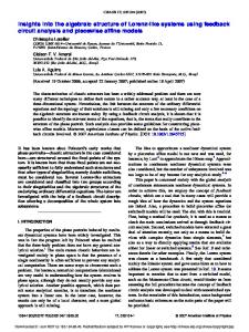
P (t) (t) For each rank k ∈ {1, 2, . . . 25}, we plot the average capture rate φ¯ k := T1 Tt=1 φ(Uk , V2 ) over T = 50 repeated trials in Figure .. Notice that when k = 1, φ¯ k is already between 0.420 and 0.673. For k ≥ 2 on the other hand, the increase from φ¯ k−1 to φ¯ k is relatively small. We found that the values {v · u1 }v∈V2 all have the same sign , whereas for i ≥ 2, the values {v · ui }v∈V2 are more evenly distributed around . Figure . shows the distribution {v · ui }v∈V2 for i = 1 and i = 2; the distribution {v · ui }v∈V2 for i ≥ 2 is similar to the distribution for i = 2.
.
Conclusion
Our results show that the subspace of many categories and relations are low-dimensional. Moreover, we demonstrated that the first basis u1 is the “defining” vector that encodes the most general information about a category c (or a relation r): Letting v = vw for any w ∈ Dc (or v = va − vb for any (a, b) ∈ Dr ), the first coordinate v · u1 has the largest magnitude, and the sign of v · u1 is always positive. All other subsequent basis vectors ui for i ≥ 2 encode more “specific” information pertaining to individual words in Dc (or word pairs in Dr ). It remains to be discovered what specific features are captured by these basis vectors for various categories and relations. For example, if Uk is a basis for the subspace of category c = country, For each trial t ∈ {1, . . . , T }, φ(U (t) , V (t) ) is the capture rate attained in trial t, where V (t) = {v : w ∈ S (t) } is the set of w 2 2 2 k (t) (t) vectors for words in the testing set S2 (which is randomly generated in Step ), and Uk is the rank-k basis computed in
Step . Recall that, in Step of Algorithm ., we scale u by ±1 so that P 1 v∈V1 v · u1 > 0.
On the Linear Structure of Word Embeddings
Chapter . Low-rank subspaces |
then perhaps having a positive second coordinate vw · u2 in the basis indicates that w is a developed country, and having a negative fourth coordinate vw · u4 indicates that country w is located in Europe. We leave this to future work.
Chapter . Low-rank subspaces |
On the Linear Structure of Word Embeddings
category
0.9
animal music_genre 0.8
musical_instrument organism_classification politician
φk
0.7
religion sport tourist_attraction
0.6
country capital_city currency
0.5
language 0.4 0
5
10
15
20
25
k
0.8
0.7
relation capital_country currency_used
φk
country_language 0.6
country−capital2 city−in−state
0.5
0
5
10
15
20
25
k
Figure .: Results from the experiment in Section .., where we use cross-validation over T = 50 repeated trials to assess how much the low-rank basis Uk returned by GET_BASIS (Algorithm .) captures the subspace of a category c (or a relation r). In each trial t ∈ {1, . . . , T }, we randomly (t) (t) (t) split Vc (or Vr ) into a training set V1 and a testing set V2 , then compute a rank-k basis Uk (t)
for the subspace spanned by V1 . For each rank k ∈ {1, 2, . . . 25}, we plot the average capture rate P (t) (t) φ¯ k := T1 Tt=1 φ(Uk , V2 ) (.), where a higher capture rate means that the vectors in V2 have a large projection onto Uk . When rank is k = 1, φ¯ k is already between 0.420 and 0.673. For ranks k ≥ 2 on the other hand, the increase from φ¯ k−1 to φ¯ k is relatively small. This shows that the first basis vector u1 is the “defining” vector that encodes the most information about a category c (or a relation r).
Chapter . Low-rank subspaces |
On the Linear Structure of Word Embeddings
cheese u1
u1
animal
u2
u2
● ●
−1.0
−0.5
0.0
0.5
1.0
●
−1.0
−0.5
0.5
1.0
0.5
1.0
0.5
1.0
0.5
1.0
0.5
1.0
0.5
1.0
u1
country
u1
cocktail
0.0
●
u2
u2
●
−1.0
−0.5
0.0
0.5
1.0
−1.0
−0.5
languages u1
u1
currency
0.0
u2
u2
●● ●
−1.0
−0.5
0.0
0.5
1.0
−1.0
−0.5
u2
u2
u1
music_genre
u1
musical_instrument
0.0
−1.0
−0.5
0.0
0.5
1.0
−1.0
−0.5
u2
u2
u1
politician
u1
organism_group
0.0
−1.0
−0.5
0.0
0.5
1.0
−1.0
−0.5
●
−1.0
u2
u2
u1
sport
u1
religion
0.0
●●
−0.5
0.0
0.5
1.0
0.5
1.0
−1.0
−0.5
0.0
u2
u1
tourist_attraction
●● ● ● ●
−1.0
−0.5
●
0.0
Figure .: For various categories c from Figure ., we randomly split Vc into a training set V1 and a testing set V2 , then compute a rank-k basis Uk = {u1 , u2 , . . . , uk } for the subspace spanned by V1 . Here, we provide a boxplot of the distribution of {v · u1 }v∈V2 (denoted by u) and the distribution of {v · u2 }v∈V2 (denoted by u). Note that for each category c, we have v · u1 > 0 for all v ∈ V2 , whereas {v · u2 }v∈V2 is more evenly distributed around . The distribution of {v · ui }v∈V2 for i ≥ 2 is similar to the distribution for i = 2, so we omit them here.
Chapter . Low-rank subspaces |
On the Linear Structure of Word Embeddings
●
●
●
u2
● ●● ●● ● ●●●●
u2
●
city−in−state u1
u1
capital_country
−1.0
−0.5
0.0
0.5
1.0
−1.0
−0.5
0.5
1.0
0.5
1.0
country_language u1
u1
country−capital2
0.0
u2
u2
●
−1.0
−0.5
0.0
0.5
1.0
0.5
1.0
−1.0
−0.5
0.0
u1
currency_used
●●●
u2
●● ● ●
−1.0
−0.5
0.0
Figure .: For various relations r from Figure ., we randomly split Vr into a training set V1 and a testing set V2 , then compute a rank-k basis Uk = {u1 , u2 , . . . , uk } for the subspace spanned by V1 . Here, we provide a boxplot of the distribution of {v · u1 }v∈V2 (denoted by u) and the distribution of {v · u2 }v∈V2 (denoted by u). Note that for eachrelation r, we have v · u1 > 0 for all v ∈ V2 (except for one outlier in r = capital_country, and one outlier in r = city-in-state), whereas {v · u2 }v∈V2 is more evenly distributed around . The distribution of {v · ui }v∈V2 for i ≥ 2 is similar to the distribution for i = 2, so we omit them here.
Chapter
Extending a knowledge base Let KB denote the current knowledge base, which consists of facts about the world that the machine currently knows. We assume that KB is incomplete, and that there are new facts to be learned. In other words, there exists categories c such that KB only knows a subset Sc ⊂ Dc of words that belong to c, and similarly, there exists relations r such that KB only knows a subset Sr ⊂ Dr of word pairs that satisfy r. Our goal is to discover new facts outside KB, such as words in D\Sc that also belong to the category c, or word pairs in (D × D)\Sr that also satisfy the relation r. In Section ., we provide an algorithm called EXTEND_CATEGORY for discovering words in D\Sc that also belong to c (see Algorithm .). Table . lists the top words returned by EXTEND_CATEGORY for various categories, and shows that the algorithm performs very well. Then in Section ., we present an algorithm called EXTEND_RELATION for discovering new word pairs in (D × D)\Sr that also satisfy r (see Algorithm .). Its accuracy for returning correct word pairs is provided in Figure .. We demonstrate that the low-dimensional subspace of categories and relations can be used to discover new facts with fairly low false-positive rates. The performance of EXTEND_RELATION (Algorithm .) is especially surprising, given the simplicity of the algorithm and the fact that it returns plausible word pairs out of all |D|(|D| − 1) ≈ 3.6e+09 possible word pairs in D × D.
.
Motivation
In Socher et. al’s paper [], a neural tensor network (NTN) model is used to learn semantic word vectors that can capture relationships between two words. More specifically, their NTN model computes a score of how plausible a word pair (a, b) satisfies a certain relationship r by the following function: " # ! va [1:m] T g(va , r, vb ) = b · f va Wr vb + θr + cr (.) vb where va , vb ∈ Rd are the vector representations of the words a, b respectively, f = tanh is a sigmoid [1:m] function, and Wr ∈ Rd×d×m is a tensor. The remaining parameters for relation r are the standard form of a neural network: θr ∈ Rm×2d and b, cr ∈ Rm . With this model, however, we see a potential danger of overfitting the data because the number [1:m] of parameters in the term vaT Wr vb in (.) is quadratic in d. Hence, our motivation is to employ
On the Linear Structure of Word Embeddings
Chapter . Extending a knowledge base |
function EXTEND_CATEGORY(Sc , k, δ): Returns a set of words in D\Sc . Inputs: • A subset Sc ⊂ Dc of words that belong to some category c • k ∈ N, the rank of the basis for the subspace of category c • δ ∈ [0, 1], a threshold value Step . Compute a rank-k basis Uk ∈ Rd×k for the subspace of category c using Algorithm .: Uk ← GET_BASIS({vw : w ∈ Sc }, k). Let u1 be the first (column) basis vector of Uk . Step . Return the set of words w ∈ D\Sc whose vectors have (i) a positive first coordinate vw · u1 in the basis Uk , and (ii) a large enough projection kvw Uk k > δ in the subspace of category c: {w ∈ D\Sc : vw · u1 > 0, kvw Uk k > δ} . end function Algorithm .: EXTEND_CATEGORY(Sc , k, δ) returns a set of words in D\Sc which are likely to belong to category c. the linear structure of the word embeddings to fit a more general model. The low-dimensional subspace of categories, as demonstrated in Chapter , gives rise to a simple algorithm that allows one to discover new facts that are not in KB.
.
Learning new words in a category
Let c be a category such that KB only knows a subset Sc ⊂ Dc of words that belong to c. We provide a method called EXTEND_CATEGORY (Algorithm .) for discovering new words in D\Sc that also belong to c.
.. Performance We tested EXTEND_CATEGORY(Sc , k, δ) on various categories c from Figure ., using rank k = 10 and threshold δ = 0.6. Table . lists the top words returned by the algorithm, where the words w ∈ D\Sc are ordered in descending magnitude of the projection kvw Uk k onto the subspace Uk of category c. The algorithm makes a few mistakes, e.g., it returns london as a tourist_attraction, and aren as a basketball_player. But overall, the algorithm seems to work very well and returns correct words that belong to the category.
On the Linear Structure of Word Embeddings (a) c = classical_composer
projection . . . . .
word schumann beethoven stravinsky liszt schubert
(c) c = university
word cambridge_university university_of_california new_york_university stanford_university yale_university
projection . . . . .
projection . . . . .
(g) c = holiday
word diwali christmas passover new_year rosh_hashanah
projection . . . . .
(i) c = animal
word horses moose elk raccoon goats
projection . . . . .
(b) c = sport
word biking volleyball skiing softball soccer
projection . . . . .
(d) c = basketball_player
(e) c = religion
word christianity hinduism taoism buddhist judaism
Chapter . Extending a knowledge base |
word dwyane_wade aren kobe_bryant chris_bosh tim_duncan
projection . . . . .
(f) c = tourist_attraction
word metropolitan_museum_of_art museum_of_modern_art london national_gallery tate_gallery
projection . . . . .
(h) c = month
word august april october february november
projection . . . . .
(j) c = asian_city
word taipei taichung kaohsiung osaka tianjin
projection . . . . .
Table .: Given a set Sc ⊂ Dc of words belonging to a category c, EXTEND_CATEGORY (Algorithm .) returns new words in D\Sc which are also likely to belong to c. Here, we list the top words returned by EXTEND_CATEGORY(Sc , k, δ) for various categories c in Figure ., using rank k = 10 and threshold δ = 0.6. The words w ∈ D\Sc are ordered in descending magnitude of the projection kvw Uk k onto the category subspace. The algorithm makes a few mistakes, e.g., it returns london as a tourist_attraction, and aren as a basketball_player. But overall, the algorithm seems to work very well, and returns correct words that belong to the category.
On the Linear Structure of Word Embeddings
.
Chapter . Extending a knowledge base |
Learning new word pairs in a relation
Let r be a well-defined relation such that KB only knows a subset Sr ⊂ Dr of word pairs that satisfy r. We now present a method called EXTEND_RELATION (Algorithm .) for discovering new word pairs in (D × D)\Sr that also satisfy r.
.. Experiment We tested EXTEND_RELATION on three well-defined relations from Figure .: capital_city, city_in_state, and currency_used. For each of the relations r, let Sr ⊆ Dr be the set of word pairs contained in the corresponding relation file (see Figure .(f)-(h)). We used cross-validation to assess the accuracy rate of Algorithm ., as follows. For each rank k ∈ {1, 2, . . . , 9} and threshold δ ∈ {0.4, 0.45, . . . , 0.75}, we repeated the following experiment over T = 50 trials: Step . Randomly partition Sr into a training set S1 and a testing set S2 , where the training set size is |S1 | = 0.3|Sr |. Let A := {a : (a, b) ∈ S2 } and B := {b : (a, b) ∈ S2 }. Step . Use Algorithm . to find a set S of word pairs in (D × D)\S1 which are likely to satisfy relation r: S ← EXTEND_RELATION(S1 , {k, k, k}, {δ, δ, δ}). Step . Let S 0 := {(a, b) ∈ S : a ∈ A or b ∈ B}. For each answer (a, b) ∈ S 0 , we count it as correct if (a, b) ∈ S2 , and incorrect otherwise. So the resulting accuracy of EXTEND_RELATION using parameters k and δ is acc(k, δ) :=
# correct answers |S 0 ∩ S2 | = . # total answers |S 0 |
.. Performance For each rank k ∈ {1, 2, . . . , 9} and threshold δ ∈ {0.4, 0.45, 0.5, . . . , 0.75}, we plot the average accuracy 1 PT (t) t=1 acc (k, δ) over T = 50 trials in Figure .a. The table in Figure .b lists the parameters T k and δ that attained the highest average accuracy. The algorithm achieved significantly higher accuracy for r = capital_city than for the other two relations; we discuss why in Section ... However, the performance of EXTEND_RELATION is still quite remarkable, considering the fact that � it returns reasonable word pairs out of the |D| 2 ≈ 1.8e+09 possible word pairs in D × D. As the threshold δ is increased, the algorithm filters out more words in Step and word pairs in Step of the algorithm, resulting in a smaller number of word pairs returned by the algorithm. Figure . illustrates this effect for r = capital_city. Note that the algorithm’s accuracy can be further improved by fine-tuning the parameters. In our experiment (Section ..), we used the same rank k for kA , kB , and kr , and also used the same threshold δ for δA , δB , and δr ; but one can vary each of these parameters separately to achieve better performance. We ignore the answers (a, b) ∈ S such that a < A and b < B, because we do not have an automated way of determining whether it is correct or incorrect. One could check each of these answers manually using an external knowledge source (e.g., Google search), but doing so would be very time-consuming. where acc(t) (k, δ) is the accuracy obtained in trial t.
On the Linear Structure of Word Embeddings
Chapter . Extending a knowledge base |
function EXTEND_RELATION(Sr , {kA , kB , kr }, {δA , δB , δr }): Returns a set of word pairs in (D × D)\Sr . Inputs: • A subset Sr ⊂ Dr of word pairs that satisfy some well-defined relation r. Let A := {a : (a, b) ∈ Sr } and B := {b : (a, b) ∈ Sr }. Let cA be the category such that, for all a ∈ A, a belongs to category cA . Similarly, let cB be the category such that, for all b ∈ B, b belongs to category cB . • kA , kB , kr ∈ N, the rank of the basis for the subspaces of cA , cB , and r respectively • δA , δB , δr ∈ [0, 1], threshold values Step . Use Algorithm . to get a set of words SA ⊆ D\A whose vectors have a large enough projection (≥ δA ) in the rank-kA subspace of category cA , and a set of words SB ⊆ D\B whose vectors have a large enough projection (≥ δB ) in the rank-kB subspace of category cB : SA ← EXTEND_CATEGORY(A, kA , δA ) SB ← EXTEND_CATEGORY(B, kB , δB ). Step . Compute a rank-kr basis for the subspace of relation r using Algorithm .: Ukr ← GET_BASIS({va − vb : (a, b) ∈ Sr }, kr ). Let u1 be the first (column) basis vector of Ukr . Step . Return the set of word pairs (a, b) ∈ SA × SB whose difference vectors have (i) a positive first coordinate (va − vb ) · u1 in the basis Ukr , and (ii) a large enough projection k(va − vb )Ukr k > δr in the subspace of relation r: {(a, b) ∈ SA × SB : (va − vb ) · u1 > 0, k(va − vb )Uk k > δr } . end function Algorithm .: EXTEND_RELATION(Sr , {kA , kB , kr }, {δA , δB , δr }) returns a set of word pairs (a, b) ∈ (D × D)\Sr which are likely to satisfy relation r.
On the Linear Structure of Word Embeddings
Chapter . Extending a knowledge base |
.. Varying levels of difficulty for different relations We provide two explanations as to why EXTEND_RELATION underperforms on relations such as city_in_state and currency_used: . For r = capital_city, there is a one-to-one mapping between the sets Ar := {a : (a, b) ∈ Sr } and Br := {b : (a, b) ∈ Sr }, whereas the same does not hold for r = city_in_state or r = currency_used (see Figure .). This causes the algorithm to return many false-positive answers for the relations city_in_state and currency_used, as we illustrate with an example below. Consider the relation r = currency_used. In the set Sr of word pairs contained in the relation file for r (see Figure .(h)), there are country-currency pairs (a, b) ∈ Sr where b = franc. For of these pairs {(a, franc) ∈ Sr }, the country word a belongs to the category c = african_country. Because the low-rank basis Ukr for relation r (computed in Step of Algorithm .) tries to capture the vectors in the set {va − vfranc : (a, franc) ∈ Sr }, and the vectors of words belonging to the category c = african_country are clustered together, the algorithm returns many false-positive pairs consisting of an African country and the currency franc. For example, in many trial runs, the algorithm returns incorrect pairs such as (kenya, franc), (uganda, franc), and (sudan, franc). False-positive answers such as these cause the algorithm’s accuracy to drop. . Some relations are just inherently more difficult than others to represent using word vectors. For example, Figure . shows that solving analogy queries of the form “a:b::c:??” for pairs (a, b), (c, d) in the relation file for country-currency is more difficult than for pairs (a, b), (c, d) satisfying the relation country-capital. This may explain why EXTEND_RELATION performs worse on currency_used than on capital_city.
. Conclusion We have demonstrated that the low-dimensional subspace of categories and relations can be used to discover new facts with fairly low false-positive rates. The performance of EXTEND_RELATION (Algorithm .) is especially surprising, given the simplicity of the algorithm and the fact that it returns plausible word pairs out of all possible word pairs in D×D. The algorithms EXTEND_CATEGORY (Algorithm .) and EXTEND_RELATION (Algorithm .) are computationally efficient, are shown to drastically narrow down the search space for discovering new facts, and can be used to supplement other methods for extending knowledge bases.
In other words, given a word a ∈ A , there exists a unique word b ∈ B such that (a, b) satisfies the relation r; and r r conversely, given a word b ∈ Br , there exists a unique word a ∈ Ar such that (a, b) satisfies r. country-currency is a smaller subset of the relation file for currency_used, and country-capital is a smaller subset of capital_city; see Figure ..
Chapter . Extending a knowledge base |
On the Linear Structure of Word Embeddings
capital_country
city−in−state
0.8
currency_used
0.8
0.8 rank−1 rank−2
0.6
accuracy
accuracy
accuracy
rank−3 0.6
rank−4
0.6
rank−5 rank−6 rank−7
0.4
0.4
0.4
0.2
0.2
0.2
0.4
0.5
0.6
δ
0.7
0.4
0.5
0.6
δ
0.7
rank−8 rank−9
0.4
0.5
0.6
δ
0.7
(a) For each rank k ∈ {1, 2, . . . , 9} and threshold δ ∈ {0.4, 0.45, . . . , 0.75}, we plot the average accuracy 1 PT acc(t) (k, δ) over T = 50 trials, where for each trial t, acc(t) (k, δ) = # correct answers is the accuracy of t=1 T # total answers (t)
(t)
the answers returned by EXTEND_RELATION(S1 , {k, k, k}, {δ, δ, δ}). (Here, each S1 ⊂ Dr is a random subset of (t)
the word pairs contained in the relation file of r (see Figure .(f)-(h)). S1 is generated randomly, at each trial t, in Step of the experiment in Section ... ).
r capital_city city_in_state currency_used
maxk,δ acc(k, δ) . . .
rank k
threshold δ . . .
(b) For each relation r, we list the parameters k and δ that achieved the highest average accuracy in (a).
Figure .: Given a set Sr ⊂ Dr of word pairs satisfying a relation r, EXTEND_RELATION (Algorithm .) returns new word pairs in (D × D)\Sr which are also likely to satisfy relation r. We use crossvalidation to assess the accuracy rate of EXTEND_RELATION on three well-defined relations from Figure .(f)-(h). Note that EXTEND_RELATION performs very well on r = capital_city, achieving accuracy as high as 0.909. We discuss why the accuracy is lower for the other two relations in Section ... For details about the experiment, see Section ...
On the Linear Structure of Word Embeddings
Chapter . Extending a knowledge base |
(a) r = capital_city cA = country
cB = city
japan germany
tokyo
canada
ottawa
berlin
(b) r = city_in_state cA = city cB = us_state
trenton
new_jersey
newark san_francisco
california
los_angeles mountain_view
(c) r = currency_used cA = country algeria serbia_montenegro germany france
cB = currency dinar euro franc
Figure .: For r = capital_city, there is a one-to-one mapping between Ar := {a : (a, b) ∈ Sr } and Br := {b : (a, b) ∈ Sr }, since a country has exactly one capital city. The same does not hold for (b) or (c), however: (b) Each U.S. state contains multiple cities, and some cities in different U.S. states have identical names (e.g., both California and New Jersey have a city named Newark). (c) A country can have multiple currencies (either concurrently or over history), and the same currency can be used in multiple countries. This causes EXTEND_RELATION to return a higher number of false-positive (incorrect) answers for (b) and (c); see Section .. for a detailed explanation.
Chapter . Extending a knowledge base |
On the Linear Structure of Word Embeddings
rank−2
rank−7
rank−8
75
75
75
50
50
50
25
25
25
0
0
0
0.4
0.5
δ
0.6
0.7
0.4
0.5
δ
0.6
0.7
0.4
0.5
δ
0.6
0.7
Figure .: Let r = capital_city, and let S1 ⊂ Dr be a random subset of the word pairs contained in the relation file of r (see Figure .(g)). We plot the number of correct (blue) and incorrect (red) word pairs returned, respectively, by calling EXTEND_RELATION(S1 , {k, k, k}, {δ, δ, δ}) for varying threshold values δ (see Algorithm .). We only provide plots for the ranks k ∈ {2, 7, 8}; the plots for other ranks are similar. As the threshold δ is increased, the algorithm filters out more word pairs in Steps and of the algorithm, resulting in a smaller number of word pairs returned by the algorithm.
Chapter
Learning vectors for less frequent words Since the size of the co-occurrence data is quadratic in the size of the vocabulary D, and since the co-occurrence data for infrequent words are too noisy to generate good word vectors with, we restrict the vocabulary D to only the words that appear at least m0 = 1000 times in the corpus. Hence, we do not have vectors for words that appear fewer than 1000 times in the corpus. These words include the famous composer claude_debussy ( times), Malaysian currency ringgit ( times), the famous actor adam_sandler ( times), and the historical event boston_massacre ( times). In order to continually extend the knowledge base KB, it becomes necessary to learn vectors for these less frequent words. We demonstrate that, using the low-dimensional subspace of categories, one can substantially reduce the amount of co-occurrence data needed to learn vectors for words. In particular, we present an algorithm called LEARN_VECTOR (Algorithm .) for learning vectors of words with only a small amount of co-occurrence data. We test the algorithm on seven words wˆ (listed in Table .) which we already have vectors for, and compare the “true” vector vwˆ ∈ VD to the vector vˆ returned by LEARN_VECTOR. The algorithm’s performance is given in Figure .. In general, the algorithm achieves very good performance while using only a small fraction of the total amount of co-occurrence data in the Wikipedia corpus C. One can extend this method to learn vectors for any words – even words that do not appear at all in the Wikipedia corpus – using web-scraping tools, such as Google search, to obtain additional co-occurrence data.
.
Learning a new vector
Let wˆ be a word such that (i) we know the category c that wˆ belongs in, and (ii) we have a small corˆ Then we provide a method LEARN_VECTOR pus Γ (where |Γ | � |C|) containing co-occurrence data for w. for learning its word vector vˆ ∈ Rd (see Algorithm .). There are a total of 283, 847 words that occur between and times in the corpus, which are not included in D.
On the Linear Structure of Word Embeddings
Chapter . Learning vectors |
ˆ c, Γ , k, η, λ): Returns a learned vector vˆ ∈ Rd for word w. ˆ function LEARN_VECTOR(w, Inputs: ˆ a word • w, • c, the category that wˆ belongs in. Let Vc := {vw : w ∈ Dc } be the vectors of words belonging to c. • Γ , a small corpus containing co-occurrence data for wˆ • k ∈ N, the rank of the basis for the category subspace • η ∈ (0, 1], the learning rate for Adagrad • λ > 0, the weight of the regularization term in the objective (.) Step . Compute a rank-k basis Uk ∈ Rd×k for the subspace of category c using Algorithm .: Uk ← GET_BASIS(Vc , k). Step . Consider only the set D 0 of vocabulary words that appear at least m00 = 10 times in Γ . For each word w ∈ D 0 , compute Yww ˆ , the number of times word w appears in any context window around wˆ in Γ . Step . Use Adagrad with learning rate η to train parameters vˆ ∈ Rd , b ∈ Rk , and Z ∈ R so as to minimize the objective X
� �2 2 2 g(Yww ˆ ) ||vˆ + vw || − log(Yww ˆ ) + Z + λkvˆ − Uk bk ,
(.)
w∈D 0 ∩D
where {vw }w∈D are the already-learned word vectors, and g(x) := min
��
� x 0.75 ,1 10
� . Note
ˆ b, and Z are initialized randomly. that v, ˆ = 1. Step . Normalize vˆ so that kvk ˆ the learned word vector for w. ˆ Step . Return v, end function ˆ c, Γ , k, η, λ) returns a vector vˆ ∈ Rd for word wˆ learned using the Algorithm .: LEARN_VECTOR(w, objective (.).
Chapter . Learning vectors |
On the Linear Structure of Word Embeddings wˆ california christianity germany hinduism japan massachusetts princeton
c us_state religion country religion country us_state university
k
Xwˆ .e+ .e+ .e+ .e+ .e+ .e+ .e+
Table .: In the experiment, we train vectors for the words wˆ by minimizing the objective (.). c is the category that wˆ belongs in. For the words california, germany, and japan, we used k = 10 as the P rank of the basis of the category subspace; for the remaining four words, we used rank k = 3. ˆ in the original corpus C. Xwˆ := w∈C Xww ˆ measures the amount of co-occurrence data for w
.. Motivation behind the optimization objective The objective (.) is nearly identical to the Squared Norm (SN) objective (.), except for a few differences: (i) we have an additional regularization term λkvˆ − Uk bk2 , (ii) the co-occurrence counts 0 Yww ˆ are taken from the smaller corpus Γ , and (iii) the summation is taken over words w ∈ D ∩ D. 2 Note that b has a closed-form solution, since to minimize kvˆ − Uk bk , one can just take b to be the projection of vˆ onto Uk . The regularization term λkvˆ − Uk bk2 serves as a prior knowledge, forcing the new vector vˆ to be trained near the subspace Uk of category c, but also allowing vˆ to lie outside the subspace. The hope is that the regularization term reduces the amount of co-occurrence data ˆ Note that in general, the regularization weight λ should be decreasing in the size needed to fit v. of Γ , since less prior knowledge is needed with more data.
.
Experiment
For our experiment, we chose seven words wˆ (listed in Table .) which we already have vectors for, fitted a vector vˆ using LEARN_VECTOR (Algorithm .), and compared vˆ to the true vector vwˆ ∈ VD (see Figure .). We withheld the true vector vwˆ ∈ VD from training, by taking wˆ out of the summation over D 0 ∩ D in the objective (.). For the words california, germany, and japan, we used k = 10 as the rank of the basis of the category subspace; for the remaining four words, we used rank k = 3. P ˆ we use Ywˆ (Γ ) := w∈D 0 Yww For each word w, ˆ to quantify the amount of co-occurrence data for word wˆ in a corpus Γ with vocabulary set D 0 , and evaluate the algorithm in Section . for varying values of Ywˆ (Γ ). More specifically, we extracted six subcorpora Γ1 , . . . , Γ6 from the original corpus C, where Γ1 ⊂ Γ2 ⊂ · · · ⊂ Γ6 ⊂ C and Ywˆ (Γ1 ) < Ywˆ (Γ2 ) < · · · < Ywˆ (Γ6 ) � Ywˆ (C) = Xwˆ . For each i ∈ {1, . . . , 6}, we ran the algorithm with various learning rates ηi and regularization weights λi ; Table . lists the parameter values that resulted in the best performance for each corpus size and each word.
.
Performance
We evaluate the performance of LEARN_VECTOR by considering the order and the cosine score of the learned vector vˆ returned by the algorithm, defined below.
On the Linear Structure of Word Embeddings
Chapter . Learning vectors |
.. Order and cosine score of the learned vector Let wˆ be one of the seven words we trained a vector for, vˆ the learned vector returned by the ˆ Number the vectors v1 , v2 , . . . , v|D| ∈ VD in algorithm, and vwˆ ∈ VD the “true” vector for word w. ˆ so that v1 · vˆ > v2 · vˆ > · · · > v|D| · v. ˆ Then the order of vˆ order of decreasing cosine similarity from v, is the number k ∈ N such that vwˆ = vk , i.e., the true vector vwˆ has the kth largest cosine similarity from vˆ out of all the words in D. The cosine score of vˆ is the cosine similarity between the true ˆ vector vwˆ and the vector vˆ returned by the algorithm, i.e., vwˆ · v.
.. Evaluation In Figure .,Pwe provide a plot of the order and cosine score of vˆ for varying values of ln(Ywˆ ), ˆ in the training corpus Γ with where Ywˆ := w∈D 0 Yww ˆ is the amount of co-occurrence data for w vocabulary set D 0 . Note that in general, the order of vˆ is decreasing, and the cosine score of vˆ is increasing, in the amount of co-occurrence data Ywˆ . Moreover, the algorithm seems to achieve a higher cosine score by using a smaller rank k for the basis of the category subspace: The words for which rank k = 10 was used (california, germany, and japan) have lower cosine scores than the words for which rank k = 3 was used. We provide an explanation as to why using a smaller rank k improves the algorithm’s performance. For a category c, let Uk be a rank-k basis for the subspace of c. The regularization term λkv − Uk bk in the objective (.) serves to train vˆ near the subspace Uk , which by definition only captures the general notion of category c. Recall from Chapter that the first basis vector u1 of Uk is the defining vector that encodes the most information about c, while the subsequent basis vectors ui for i ≥ 2 capture more specific information about individual words in c. By using a smaller rank k, we throw away the more “noisy” vectors ui for i ≥ k ≥ 1, allowing Uk to capture the generation notion of category c better. This allows the regularization term to train the “category” component of vˆ more accurately. Note that the other component, which is specific to word wˆ and lies outside � �2 the category subspace, is trained by the term g(Yww0 ) ||v + vw0 ||2 − log(Yww0 ) + Z in the objective (.). ˆ one using a low rank k and To illustrate our point, we trained two vectors for the same word w, the other using a high rank k, and compared their order and cosine score (see Figure .). For both wˆ = massachusetts and wˆ = hinduism, the vector learned using the lower rank resulted in a lower order and a much higher cosine score. This demonstrates that using a smaller rank k results in better performance for LEARN_VECTOR. To compare the amount of co-occurrence data for wˆ in a subcorpus Γ to the amount of cooccurrence data for wˆ in the Wikipedia corpus C, we look at the fraction Ywˆ (Γ )/Xwˆ , which is listed in Table .. Note that the algorithm achieves very good performance while using only a small fraction of the total amount of co-occurrence data in the Wikipedia corpus C. For example, by using only Ywˆ (Γ )/Xwˆ = 1.846e − 02 of the total amount of co-occurrence data for the word w = christianity, the algorithm is able to learn a vector whose order is and cosine score is 0.84. Lastly, note that the performance depends heavily on the parameter values chosen, and can be further improved by fine-tuning the parameters.
Chapter . Learning vectors |
On the Linear Structure of Word Embeddings
30
0.8 word
cosine score
california
order
20
christianity germany
0.7
hinduism japan massachusetts
10
princeton
0.6
0 6
7
ln(Yw^)
8
9
6
7
ln(Yw^)
8
9
Figure .: The order and cosine score of the learned vector vˆ returned by LEARN_VECTOR (Algoˆ using varying amounts of co-occurrence data Ywˆ . (See Section .. for the rithm .) for word w, definitions of order and cosine score.) Note that in general, the order of vˆ is decreasing, and the cosine score of vˆ is increasing, in the amount of co-occurrence data Ywˆ . (The occasional decrease ˆ Also, observe that the words in the cosine score is due to random initialization of the vector v.) for which rank k = 10 was used (california, germany, and japan) have lower cosine scores than the words for which rank k = 3 was used. The algorithm achieves very good performance while using only a small fraction of the total amount of co-occurrence data in the Wikipedia corpus C: For example, by using only Ywˆ (Γ )/Xwˆ = 1.846e−02 of the total amount of co-occurrence data for the word w = christianity, the algorithm is able to learn a vector whose order is and cosine score is 0.84.
.
Conclusion
We have demonstrated that, in principle, one can learn vectors with substantially less data by using the low-dimensional subspace of categories. An interesting experiment to try is the following: Use Algorithm . to learn vectors for rare words, and see if new facts can be discovered using these vectors. We leave this to future work. Moreover, one can extend this method to learn vectors for any words – even words that do not appear at all in the Wikipedia corpus – using web-scraping tools, such as Google search, to obtain additional co-occurrence data. However, the corpora obtained from Google search may be drawn from a different distribution than the wikipedia corpus, and hence skew the data in a certain way. We leave this to future work. One weakness of LEARN_VECTOR is that it requires having prior knowledge of what category a word wˆ belongs in. If our prior knowledge is wrong, then the fitted vector for wˆ may be very bad. One could come up with an automatic method classifying which category w belongs to.
Chapter . Learning vectors |
On the Linear Structure of Word Embeddings
(a) w = california i 1 2 3 4 5 6
ln Yw (Γi ) . . . . . .
Yw (Γi )/Xw .e- .e- .e- .e- .e- .e-
(b) w = christianity
ηi .e- .e- .e- .e- .e- .e-
λi . . . . . .
i 1 2 3 4 5 6
ln Yw (Γi ) . . . . . .
(c) w = germany i 1 2 3 4 5 6
ln Yw (Γi ) . . . . . .
Yw (Γi )/Xw .e- .e- .e- .e- .e- .e-
ln Yw (Γi ) . . . . . .
Yw (Γi )/Xw .e- .e- .e- .e- .e- .e-
ηi .e- .e- .e- .e- .e- .e-
λi . . . . . .
(d) w = hinduism
ηi .e- .e- .e- .e- .e- .e-
λi . . . . . .
i 1 2 3 4 5 6
ln Yw (Γi ) . . . . . .
(e) w = japan i 1 2 3 4 5 6
Yw (Γi )/Xw .e- .e- .e- .e- .e- .e-
Yw (Γi )/Xw .e- .e- .e- .e- .e- .e-
ηi .e- .e- .e- .e- .e- .e-
λi . . . . . .
(f) w = massachusetts ηi .e- .e- .e- .e- .e- .e-
λi . . . . . .
i 1 2 3 4 5 6
ln Yw (Γi ) . . . . . .
Yw (Γi )/Xw .e- .e- .e- .e- .e- .e-
ηi .e- .e- .e- .e- .e- .e-
λi . . . . . .
(g) w = princeton i 1 2 3 4 5 6
ln Yw (Γi ) . . . . . .
Yw (Γi )/Xw .e- .e- .e- .e- .e- .e-
ηi .e- .e- .e- .e- .e- .e-
λi . . . . . .
ˆ we extracted Table .: For each word w, P six subcorpora Γ1 , . . . , Γ6 from the original corpus C, where Γ1 ⊂ Γ2 ⊂ · · · ⊂ Γ6 . We use Ywˆ (Γ ) := w∈D 0 Yww ˆ to quantify the amount of co-occurrence data for word wˆ in a corpus Γ with vocabulary set D 0 . For each i ∈ {1, . . . , 6}, we trained the algorithm on the subcorpus Γi for various learning rates ηi and regularization weights λi . In the tables above, we list the parameter values ηi , λi that resulted in the best performance (shown in Figure .). To compare the amount of co-occurrence data for wˆ in Γ to the amount of co-occurrence data for wˆ in C, we look at the fraction Ywˆ (Γ )/Xwˆ .
Chapter . Learning vectors |
On the Linear Structure of Word Embeddings
0.8
cosine score
order
30
20
0.7 rank−10 rank−3
0.6
10 0.5
0 6
7
ln(Yw^)
8
9
6
7
ln(Yw^)
8
9
(a) wˆ = massachusetts
0.8
150
cosine score
0.7
order
100
50
rank−15
0.6
rank−3
0.5
0.4
0 6
7
ln(Yw^)
8
9
6
7
ln(Yw^)
8
9
(b) wˆ = hinduism
ˆ Figure .: Using LEARN_VECTOR (Algorithm .), we trained two vectors for the same word w, one using a low rank k (blue) and the other using a high rank k (red), and compared their order and cosine score. (For each rank k, we tried various learning rates η and regularization weights λ to try to optimize performance; here, we provide the best performance found for each k.) For both wˆ = massachusetts and wˆ = hinduism, the vector learned using the lower rank resulted in a lower order and a much higher cosine score. This demonstrates that using a smaller rank k results in better performance for LEARN_VECTOR.
Chapter
Using an external knowledge source to reduce false-positive rate One can use external knowledge sources such as a dictionary or Wordnet [] to filter false-positive answers and improve accuracy on analogy queries. In this section, we focus on analogy queries “a:b::c:??” where there exists categories cA , cB such that both a and c belong in cA , and both b and the correct answer d belong in cB . In other words, (a, b) and (c, d) both satisfy a common relation r that is well-defined. SOLVE_QUERY (Algorithm .) is a generic method for returning the top N answers to an analogy query “a:b::c:??”. In Section ., we present two ways for filtering the candidate list of answers to reduce false-positive rate: POS filter and LEX filter. Figures ., ., and . compare the accuracy of SOLVE_QUERY with and without these filters on different relations r. We show that the POS filter always increases the accuracy (either slightly or significantly, depending on the relation r), unless the accuracy is already 100% without filter. On the other hand, the performance for the LEX filter varies widely, depending on the nature of the relation r. When used on appropriate relations r, such as facts-based relations (see Figure .(a)-(h)), the LEX filter can improve the accuracy by as much as +19.2% than without filter, and +17.7% than with POS filter (see Figure .(a)).
.
Analogy queries
Recall that word embeddings allow one to solve analogy queries of the form “a:b::c:??” using simple vector arithmetics. More specifically, for two word pairs (a, b), (c, d) satisfying a common relation r, their word vectors satisfy va − vb ≈ vc − vd . Hence, a method to solve the analogy query “a:b::c:??” is to find the word d ∈ D whose vector vd is closest to vb − va + vc . Given a set of words ∆ ⊆ D and a number N ∈ {1, . . . , |∆|}, SOLVE_QUERY (Algorithm .) returns the top N answers in ∆ for the analogy query “a:b::c:??”. More specifically, it returns N words in ∆ corresponding to the top N vectors in V∆ := {vw : w ∈ ∆} that are closest to the vector vb − va + vc . It is also used in other works (e.g. [, , ]) to evaluate a method’s performance on analogy tasks.
On the Linear Structure of Word Embeddings
Chapter . Using external knowledge |
function SOLVE_QUERY({a, b, c}, ∆, N ): Returns a list of N words in ∆. Inputs: • Words a, b, c for which we want to solve the analogy query “a:b::c:??” • ∆ ⊆ D, a set of candidate answers • N ∈ {1, 2, . . . , |∆|}, the number of answers to return. Step . Let V∆ := {vw : w ∈ ∆}. Number the vectors v1 , v2 , . . . , v|∆| ∈ V∆ in order of decreasing cosine similarity from the vector vb − va + vc . Let S := {v1 , v2 , . . . , vN }. Step . Return the list {w ∈ ∆ : vw ∈ S}. end function Algorithm .: SOLVE_QUERY({a, b, c}, ∆, N ) returns top N answers from ∆ for the analogy query “a:b::c:??”. We say SOLVE_QUERY returns the correct answer if the correct answer d is in the set returned by the algorithm.
.
Wordnet
In Wordnet, each word is labeled with POS (“part-of-speech”) and LEX (“lexicographic”) tags. The POS tag indicates the syntactic category of a word, such as noun, verb, adjective, and adverb. The LEX tag is more specific: See Table . for a complete list of the LEX tags in Wordnet. For any word w ∈ D, let pos(w) and lex(w) be the set of POS and LEX tags for w, respectively. For example, for the currency word w = euro, pos(euro) = {noun}, lex(euro) = {noun.quantity}. Define the following sets: Dpos(w) := {w0 ∈ D : pos(w0 ) ∩ pos(w) , ∅}, Dlex(w) := {w0 ∈ D : lex(w0 ) ∩ lex(w) , ∅}. In other words, Dpos(w) is the set of words that share a common POS tag with w, and similarly, Dlex(w) is the set of words that share a common LEX tag with w. For example, Dpos(euro) contains all the noun words in D, and Dlex(euro) contains words such as dollar and kilometer which have the LEX tag noun.quantity. Consider the analogy query “a:b::c:??” where there exists categories cA and cB such that both a and c belong in cA , and both b and the correct answer d belong in cB . If we assume that every
Chapter . Using external knowledge |
On the Linear Structure of Word Embeddings
word in category cB share a common POS (or LEX) tag, then we can use Wordnet to filter out words in D which cannot belong in cB . More specifically, we only search among the words in Dpos(b) (or Dlex(b) ) for the correct answer d. Note that LEX is a stronger filter than POS, in the sense that Dlex(b) ⊂ Dpos(b) .
.
Experiment
We tested SOLVE_QUERY (Algorithm .) on relations from Figure . in the following manner. For each relation r, let Sr ⊂ Dr be the set of word pairs contained in the correponding relation file (see Figure .). For each N ∈ {1, 5, 10, 25, 50}, we performed the following experiment: Step . Initialize n = npos = nlex = 0. Step . For each (a, b) ∈ Sr , and for each (c, d) ∈ Sr such that (c, d) , (a, b), solve the analogy query “a:b::c:??” using Algorithm .: S ← SOLVE_QUERY({a, b, c}, D, N ) Spos ← SOLVE_QUERY({a, b, c}, Dpos(b) , N ) Slex ← SOLVE_QUERY({a, b, c}, Dlex(b) , N ). We say S, Spos , and Slex are the answers returned by the algorithm without filter, with POS filter, and with LEX filter, respectively. • If d ∈ S, then increment n by . • If d ∈ Spos , then increment npos by . • If d ∈ Slex , then increment nlex by . In other words, we test the algorithm on the analogy queries “a:b::c:??” and “c:d::a:??” for every possible pairs (a, b), (c, d) ∈ Sr . The total number of times the algorithm returns the correct answer without filter, with POS filter, and with LEX filter are n, npos , and nlex , respectively. Since the total number of analogy queries tested on is |Sr |(|Sr |−1), the accuracy of the algorithm without filter, with n nlex POS filter, and with LEX filter are given by |S |(|Sn |−1) , |S |(|Spos|−1) , and |S |(|S , respectively. |−1) r
.
r
r
r
r
r
Performance
Figures ., ., and . compare the accuracy of SOLVE_QUERY with and without filters on different relations r, which are taken from Figure .. We ignore the performance on relation (n) gram-nationality-adj in Figure ., due to the fact that Wordnet does not have an entry for the word “argentinean” which is included in the test bed. Depending on the relation r, the POS filter always increases the accuracy, either slightly (see (a), (c), (j), (l), (m), (o)-(z)) or significantly (see (i)), unless the accuracy is already 100% without filter (see (b), (d), (e), (f), (k)). So for all analogy queries “a:b::c:??” where either b or the correct answer d is the word argentinean, both POS and LEX filter out the correct answer from D, causing the algorithm to get the analogy query wrong and therefore lower its accuracy slightly.
On the Linear Structure of Word Embeddings #
LEX tag adj.all adj.pert adv.all noun.Tops noun.act noun.animal noun.artifact noun.attribute noun.body noun.cognition noun.communication noun.event noun.feeling noun.food noun.group noun.location noun.motive noun.object noun.person noun.phenomenon noun.plant noun.possession noun.process noun.quantity noun.relation noun.shape noun.state noun.substance noun.time verb.body verb.change verb.cognition verb.communication verb.competition verb.consumption verb.contact verb.creation verb.emotion verb.motion verb.perception verb.possession verb.social verb.stative verb.weather adj.ppl
Chapter . Using external knowledge |
Description all adjective clusters relational adjectives (pertainyms) all adverbs unique beginner for nouns nouns denoting acts or actions nouns denoting animals nouns denoting man-made objects nouns denoting attributes of people and objects nouns denoting body parts nouns denoting cognitive processes and contents nouns denoting communicative processes and contents nouns denoting natural events nouns denoting feelings and emotions nouns denoting foods and drinks nouns denoting groupings of people or objects nouns denoting spatial position nouns denoting goals nouns denoting natural objects (not man-made) nouns denoting people nouns denoting natural phenomena nouns denoting plants nouns denoting possession and transfer of possession nouns denoting natural processes nouns denoting quantities and units of measure nouns denoting relations between people or things or ideas nouns denoting two and three dimensional shapes nouns denoting stable states of affairs nouns denoting substances nouns denoting time and temporal relations verbs of grooming, dressing and bodily care verbs of size, temperature change, intensifying, etc. verbs of thinking, judging, analyzing, doubting verbs of telling, asking, ordering, singing verbs of fighting, athletic activities verbs of eating and drinking verbs of touching, hitting, tying, digging verbs of sewing, baking, painting, performing verbs of feeling verbs of walking, flying, swimming verbs of seeing, hearing, feeling verbs of buying, selling, owning verbs of political and social activities and events verbs of being, having, spatial relations verbs of raining, snowing, thawing, thundering participial adjectives
Table .: List of all LEX tags in Wordnet.
On the Linear Structure of Word Embeddings
Chapter . Using external knowledge |
On the other hand, the performance for the LEX filter varies widely depending on the nature of the relation r, due to the fact that LEX is a stronger filter than POS. For relations where words belonging to cB share a common LEX tag (e.g., (a), (c), (i), (j), (l), (r)-(v), (z)), LEX improves the accuracy significantly by filtering out false-positive answers. On the contrary, for relations where words belonging to cB have different LEX tags (e.g., (m), (o)-(q), (w), (y)), LEX filters out the correct answer from D, and hence worsens the accuracy significantly. When used on appropriate relations r, such as facts-based relations (see Figure .(a)-(h)), the LEX filter can improve the accuracy by as much as +19.2% than without filter, and +17.7% than with POS filter (see the plot in Figure .(a) for N = 50).
.
Conclusion
We have shown that external knowledge sources such as Wordnet can be used to improve accuracy on analogy queries, sometimes significantly, by filtering out false-positive answers. As an extension of the idea, we can apply the Wordnet filter to EXTEND_CATEGORY (Algorithm .) for learning new words in a category, or EXTEND_RELATION (Algorithm .) for learning new word pairs in a relation, to decrease the false-positive rate and improve its performance. We leave this to future work.
Chapter . Using external knowledge |
On the Linear Structure of Word Embeddings
(b) holiday−month
0.75
0.75
0.75
0.50
accuracy
1.00
0.50
0.50
0.25
0.25
0.25
0.00
0.00
0.00
0
10
20
30
40
50
0
10
20
N
30
40
50
0
(e) country−capital2
0.75
0.75
0.25
accuracy
0.75 accuracy
1.00
0.50
0.50
0.25
0.00 30 N
40
50
40
50
0.50
0.25
0.00 20
30
(f) city−in−state
1.00
10
20 N
1.00
0
10
N
(d) country−language
accuracy
(c) holiday−religion
1.00
accuracy
accuracy
(a) country−currency 1.00
0.00 0
10
20
30 N
40
50
0
10
20
30
40
50
N
Figure .: Accuracy of the algorithm without filter (green), with POS filter (blue), and with LEX filter (red) on the facts-based relation files from Figure .(a)-(f). For (a) and (c), the LEX filter improves the accuracy significantly, while the POS filter improves the accuracy only slightly. For all other relation files, the algorithm already achieves an accuracy of without filter.
Chapter . Using external knowledge |
On the Linear Structure of Word Embeddings
(j) gram2−opposite
0.75
0.75
0.75
0.50
accuracy
1.00
0.25
0.50
0.25
0.00 10
20
30
40
50
0.00 0
10
20
N
30
40
50
0
(m) gram5−present−particle
0.75
0.75 accuracy
0.75 accuracy
1.00
0.50
0.50
0.25
0.25
0.00
0.00
0.00
30
40
50
0
10
20
N
30
40
50
0
(p) gram8−plural
0.75
0.75
0.25
accuracy
0.75 accuracy
1.00
0.50
0.25
0.00 20
30 N
40
50
30
40
50
0.50
0.25
0.00 10
20
(q) gram9−plural−verbs
1.00
0.50
50
N
1.00
0
10
N
(o) gram7−past−tense
40
0.50
0.25
20
30
(n) gram6−nationality−adj
1.00
10
20 N
1.00
0
10
N
(l) gram4−superlative
accuracy
0.50
0.25
0.00 0
accuracy
(k) gram3−comparative
1.00
accuracy
accuracy
(i) gram1−adj−adv 1.00
0.00 0
10
20
30 N
40
50
0
10
20
30
40
50
N
Figure .: Accuracy of the algorithm without filter (green), with POS filter (blue), and with LEX filter (red) on the grammar-based relation files from Figure .(i)-(q). For (n), both the LEX filter and the POS filter worsen the accuracy slightly, due to the fact that Wordnet does not have an entry for the word “argentinean”. For all other relation files, POS improves the accuracy by a modest amount. LEX improves the accuracy for (i), (j), and (l), but performs very poorly for (m), (o)-(q), due to the fact that words belonging to cB have different LEX tags, causing LEX to filter out the correct answer.
Chapter . Using external knowledge |
On the Linear Structure of Word Embeddings
(s) associated−position
0.75
0.75
0.75
0.50
accuracy
1.00
0.25
0.50
0.25
0.00 10
20
30
40
50
0.00 0
10
20
N
30
40
50
0
(v) has−characteristic
0.75
0.75 accuracy
0.75 accuracy
1.00
0.50
0.50
0.25
0.25
0.00
0.00
0.00
30
40
50
0
10
20
N
30
40
50
0
(y) noun−baby
0.75
0.75
0.25
accuracy
0.75 accuracy
1.00
0.50
0.25
0.00 20
30 N
40
50
30
40
50
40
50
0.50
0.25
0.00 10
20
(z) senses
1.00
0.50
50
N
1.00
0
10
N
(x) has−skin
40
0.50
0.25
20
30
(w) has−function
1.00
10
20 N
1.00
0
10
N
(u) graded−antonym
accuracy
0.50
0.25
0.00 0
accuracy
(t) common−very
1.00
accuracy
accuracy
(r) associated−number 1.00
0.00 0
10
20
30 N
40
50
0
10
20
30 N
Figure .: Accuracy of the algorithm without filter (green), with POS filter (blue), and with LEX filter (red) on the semantics-based relation files from Figure .(r)-(z). LEX filter worsens the accuracy for (w) and (y), but improves the accuracy significantly on all other relation files. POS filter consistently improves the accuracy on all relation files.
Chapter
Conclusion We have demonstrated that the linear algebraic structure of word embeddings can be used to reduce data requirements for methods of learning facts. In particular, we demonstrated that categories and relations form a low-rank subspace Uk = {u1 , . . . , uk } in the projected space (Chapter ), and this subspace can be used to discover new facts with fairly low false-positive rates () and learn new vectors for words with substantially less co-occurrence data (Chapter ). In Chapter , we demonstrated that the first basis vector u1 of a low-rank subspace encodes the most general information about a category c (or a relation r), whereas the subsequent basis vectors ui for i ≥ 2 encode more “specific” information pertaining to individual words in Dc (or word pairs in Dr ). It remains to be discovered what specific features are captured by these basis vectors for various categories and relations. For example, if Uk is a basis for the subspace of category c = country, then perhaps having a positive second coordinate vw · u2 in the basis indicates that w is a developed country, and having a negative fourth coordinate vw · u4 indicates that country w is located in Europe. We leave this to future work. In Chapter , we used the low-dimensional subspace of categories and relations to discover new facts with fairly low false-positive rates. The performance of EXTEND_RELATION (Algorithm .) is fairly surprising, given the simplicity of the algorithm and the fact that it returns plausible word pairs out of all possible word pairs in D × D. At the very least, EXTEND_RELATION has shown to drastically narrow down the search space for discovering new word pairs satisfying a given relation, and allows for sharper classification than simple clustering. It can supplement other methods for extending knowledge bases to improve efficiency and attain even higher accuracy rates. One could also combine EXTEND_RELATION with POS and LEX filters described in Chapter , or explore other ways of utilizing external knowledge sources (e.g., a dictionary) to filter falsepositive answers. In Chapter we demonstrated that, in principle, one can learn vectors with substantially less data by using the low-dimensional subspace of categories. An interesting experiment to try is the following: Use LEARN_VECTOR to learn vectors for rare words in the Wikipedia corpus, and see if new facts can be discovered using these vectors. It would also be interesting to try variants of the objective (.), perhaps by adding the regularization term λkvˆ − Uk bk2 to other existing objectives such as GloVe []. Moreover, one can extend this method to learn vectors for any words – even words that do not appear at all in the Wikipedia corpus – using web-scraping tools, such as Google search, to obtain
On the Linear Structure of Word Embeddings
Chapter . Conclusion |
additional co-occurrence data. However, the corpora obtained from Google search may be drawn from a different distribution than the Wikipedia corpus, and hence could skew the data in a certain way. We leave this to future work.
Bibliography [] Sanjeev Arora, Yuanzhi Li, Yingyu Liang, Tengyu Ma, and Andrej Risteski. Random walks on context spaces: Towards an explanation of the mysteries of semantic word embeddings. CoRR, abs/., . [] Yoshua Bengio, Réjean Ducharme, and Pascal Vincent. A neural probabilistic language model. In T. K. Leen and T.G. Dietterich, editors, Advances in Neural Information Processing Systems (NIPS’). MIT Press, . [] Yoshua Bengio, Réjean Ducharme, Pascal Vincent, and Christian Jauvin. A neural probabilistic language model. Journal of Machine Learning Research, :–, . [] Steven Bird. NLTK: the natural language toolkit. In Proceedings of the COLING/ACL on Interactive presentation sessions, COLING-ACL ’, pages –. Association for Computational Linguistics, . [] Kurt D. Bollacker, Colin Evans, Praveen Paritosh, Tim Sturge, and Jamie Taylor. Freebase: A collaboratively created graph database for structuring human knowledge. In Proceedings of the ACM SIGMOD International Conference on Management of Data, SIGMOD , Vancouver, BC, Canada, June . [] Andrew Carlson, Justin Betteridge, Bryan Kisiel, Burr Settles, Estevam R. Hruschka, and Tom M. Mitchell. Toward an architecture for never-ending language learning. In In AAAI, . [] Danqi Chen, Richard Socher, Christopher D. Manning, and Andrew Y. Ng. Learning new facts from knowledge bases with neural tensor networks and semantic word vectors. CoRR, abs/., . [] Michael Collins. Log-linear models, . [] Ronan Collobert and Jason Weston. A unified architecture for natural language processing: deep neural networks with multitask learning. In William W. Cohen, Andrew McCallum, and Sam T. Roweis, editors, ICML, volume of ACM International Conference Proceeding Series, pages –. ACM, . [] S. Deerwester, S.T. Dumais, G.W. Furnas, T.K. Landauer, and R.A. Harshman. Indexing by latent semantic analysis. Journal of the American Society for Information Science , pages – , .
On the Linear Structure of Word Embeddings
BIBLIOGRAPHY |
[] John Duchi, Elad Hazan, and Yoram Singer. Adaptive subgradient methods for online learning and stochastic optimization. Technical Report UCB/EECS--, EECS Department, University of California, Berkeley, Mar . [] Anthony Fader, Stephen Soderland, and Oren Etzioni. Identifying relations for open information extraction. In EMNLP, pages –. ACL, . [] Yoav Goldberg and Omer Levy. wordvec explained: deriving mikolov et al.’s negativesampling word-embedding method. In arXiv preprint arXiv:., . [] Geoffrey E. Hinton. Learning distributed representations of concepts. In Proceedings of the eighth annual conference of the cognitive science society, pages –. Amherst, MA, . [] Omer Levy and Yoav Goldberg. Dependency-based word embeddings. In Proceedings of the nd Annual Meeting of the Association for Computational Linguistics (Volume : Short Papers), pages –, Baltimore, Maryland, June . Association for Computational Linguistics. [] Omer Levy and Yoav Goldberg. Linguistic regularities in sparse and explicit word representations. Baltimore, Maryland, USA, June . Association for Computational Linguistics. [] Christopher D. Manning, Prabhakar Raghavan, and Hinrich SchÃijtze. Introduction to Information Retrieval. Cambridge University Press, . [] Tomáš Mikolov, Stefan Kombrink, Lukáš Burget, Jan Černocký, and Sanjeev Khudanpur. Extensions of recurrent neural network language model. In Proceedings of the IEEE International Conference on Acoustics, Speech, and Signal Processing, ICASSP , pages –. IEEE Signal Processing Society, . [] George A. Miller. WordNet: A lexical database for English. Communications of the ACM, ():–, November . [] Andriy Mnih and Geoffrey E. Hinton. A scalable hierarchical distributed language model. In D. Koller, D. Schuurmans, Y. Bengio, and L. Bottou, editors, Advances in Neural Information Processing Systems , pages –. Curran Associates, Inc., . [] Andriy Mnih and Koray Kavukcuoglu. Learning word embeddings efficiently with noisecontrastive estimation. In C.J.C. Burges, L. Bottou, M. Welling, Z. Ghahramani, and K.Q. Weinberger, editors, Advances in Neural Information Processing Systems , pages –. Curran Associates, Inc., . [] David Nadeau and Satoshi Sekine. A survey of named entity recognition and classification. Lingvisticae Investigationes, ():–, . [] Jeffrey Pennington, Richard Socher, and Christopher Manning. Glove: Global vectors for word representation. In Proceedings of the Conference on Empirical Methods in Natural Language Processing (EMNLP), pages –. Association for Computational Linguistics, . [] David E. Rumelhart, Geoffrey E. Hinton, and Ronald J. Williams. Neurocomputing: Foundations of research. chapter Learning Representations by Back-propagating Errors, pages –. MIT Press, Cambridge, MA, USA, .
On the Linear Structure of Word Embeddings
BIBLIOGRAPHY |
[] Holger Schwenk. Continuous space language models. Comput. Speech Lang., ():–, July . [] Fabrizio Sebastiani. Machine learning in automated text categorization. ACM COMPUTING SURVEYS, :–, . [] Rion Snow, Daniel Jurafsky, and Andrew Y. Ng. Learning syntactic patterns for automatic hypernym discovery. In Lawrence K. Saul, Yair Weiss, and Léon Bottou, editors, Advances in Neural Information Processing Systems , pages –. MIT Press, Cambridge, MA, . [] Richard Socher, John Bauer, Christopher D. Manning, and Andrew Y. Ng. Parsing With Compositional Vector Grammars. In ACL. . [] F. M. Suchanek, G. Kasneci, and G. Weikum. Yago: a core of semantic knowledge. Proceedings of the th international conference on World Wide Web, pages –, . [] Tomas Mikolov, Ilya Sutskever, Kai Chen, Greg S. Corrado, and Jeff Dean. Distributed representations of words and phrases and their compositionality. In Advances in Neural Information Processing Systems, pages –, .