on the linear weighted sum method for multi-objective

ˇ FACTA UNIVERSITATIS (NIS) S. M. I. 26 (2011), 49–63

ON THE LINEAR WEIGHTED SUM METHOD FOR MULTI-OBJECTIVE OPTIMIZATION ∗ Ivan P. Stanimirovi´c, Milan Lj. Zlatanovi´c, Marko D. Petkovi´c

Abstract. A method providing the efficient way of construction of weighted coefficients for linear weighted sum method is provided. By applying this method, all of the resulting points are Pareto optimal points of the corresponding multi-objective optimization problem. A method for the efficient construction of weighting coefficients wi > 0 in programming package MATHEMATICA is presented. Run-time symbolic transformations of the objective functions and constraints into the corresponding single-objective constrained problem are emphasized. The implementation details and the graphical representations of two and three variables case are given, in order to depict the introduced method.

1. Introduction

Pareto optimal solutions denote a concept in economics with some applications in engineering and social sciences. Informally, Pareto efficient situations are those in which it is impossible to make one person better off without necessarily making someone else worse off. The general multi-objective optimization problem is posed as follows. We consider an ordered sequence of real objective functions with a set of constrains:

(1.1)

Maximize:

Q(x) = [Q1 (x), . . . , Ql (x)],

Subject to:

fi (x) ≤ 0, i = 1, . . . , m hi (x) = 0, i = 1, . . . , k.

x ∈ Rn

The feasible design space (often called the constraint set) in (1.1) we simply denote by X. Therefore, the set X is defined by X = {x| fi (x) ≤ 0, i = 1, . . . , m; hi (x) = 0, i = 1, . . . , k}. In the sequel, the notation x ∈ X will mean that x satisfies inequality and Received March 23, 2011. 2010 Mathematics Subject Classification. Primary 90C29; Secondary 90C05 ∗ The authors were supported in part by research project 174013 of the Serbian Ministry of Science.

49

50

I.P. Stanimirovi´c, M.Lj. Zlatanovi´c, M.D. Petkovi´c

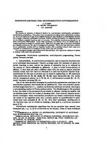
equality constraints in (1.1). By xj ∗ we denote the point that maximizes the jth objective function subject to constraints in (1.1). For the sake of completeness we restate the definitions of some types of noninferior (Pareto-optimal) solutions and ideal (utopia) point from [1], [4] and [7]. Definition 1.1. A solution x∗ is said to be Pareto optimal solution of multiobjective optimization problem (1.1) iff there does not exist another feasible solution x ∈ X such that Q j (x) ≥ Q j (x∗ ) for all j = 1, . . . , l, and Q j (x) > Q j (x∗ ) for at least one index j.

F. 1.1: Representation of the region containing Pareto optimal points All Pareto optimal points lie on the boundary of the feasible criterion space X. Often, algorithms provide solutions that may not be Pareto optimal but may satisfy other criteria, making them significant for practical applications. For instance, weakly Pareto optimal is defined as follows: Definition 1.2. A solution x∗ is said to be weakly Pareto optimal solution of multi-objective optimization problem (1.1) iff there does not exist another feasible solution x ∈ X such that Q j (x) > Q j (x∗ ) for all j = 1, . . . , l. A solution is weakly Pareto optimal if there is no other point that improves all of the objective functions simultaneously. In contrast, a point is Pareto optimal if there is no other point that improves at least one objective function without detriment to another function. It is obvious that each Pareto optimal point is weakly Pareto optimal, but weakly Pareto optimal point is not Pareto optimal. All Pareto optimal points may be categorized as being either proper or improper. The idea of proper Pareto optimality and its relevance to certain algorithms is discussed in [3] and [4]. It is defined as follows: Definition 1.3. A solution x∗ ∈ X is said to be properly Pareto optimal solution (in the sense of Geoffrion [3]) if it is Pareto optimal and there is some real number M > 0 such that for each Q j (x), x ∈ X satisfying Q j (x) > Q j (x∗ ) for all j = 1, . . . , l, there exist at least one Qi (x) such that Qi (x∗ ) > Qi (x) and optimal point is not proper called improper.

Q j (x∗ )−Q j (x) Qi (x)−Qi (x∗ )

≤ M. If a Pareto

On the linear weighted sum method for multi-objective optimization

51

A few functions for constrained numerical optimization are available in the programming package MATHEMATICA (see [5], [10]). Functions Maximize and Minimize allow to specify an objective function to maximize or minimize, together with a set of constrains. In all cases it is assumed that the variables are constrained to have non-negative values. Minimize[f, {cons}, {x, y,...}] or Minimize[{f, cons}, {x, y,...}], minimize f in the region specified by the constraints cons; Maximize[f, {cons}, {x, y,...}] or Maximize[{f, cons}, {x, y,...}], find the maximum of f , in the region specified by cons. Minimize and Maximize can in principle solve any polynomial programming problem in which the objective function f and the constraints cons involve arbitrary polynomial functions of the variables [10]. An important feature of Minimize and Maximize is that they always find global minima and maxima [10]. The main idea in the weighted sum method is to choose the weighting coefficients ωi corresponding to objective functions Qi (x), i = 1, l.. So, the multi-criteria optimization problem is transformed to a single-objective one. Many authors have developed systematic approaches to selecting weights. One of difficulties with the weighted sum method is that varying the weights consistently and continuously may not necessarily result in an accurate, complete representation of the Pareto optimal set. Also, some drawbacks of minimizing weighted sums of objectives in multi-criteria optimization problems were observed in [2]. Our motivation is to develop a specific conditions for the weighted coefficients, such that each solution gained by the linear weighted sum method is Pareto optimal. A goal is to provide a practical criteria for the construction of the weighted coefficients, in order to generate the Pareto set efficiently. Therefore, we want to use the benefits of symbolic computation of MATHEMATICA to depict the generated Pareto set and the feasible design space. This will give the better insight in the multi-objective decision making process and the position of the Pareto optimal points on the boundary of the feasible solutions set. The paper is organized as follows. In the second section we observe the properties of linear weighted sum method and provide the conditions under which the gained solution of MOO problem is Pareto optimal. Therefore, the practical method for the construction of the weighted coefficients is presented. Some implementation details for the two variables case are depicted in the third section, as well as some illustrative examples. In the last section we give the implementation details for the three variables case and observe two 3D multi-objective optimization problems, which are graphically represented via the programming package MATHEMATICA.

52

I.P. Stanimirovi´c, M.Lj. Zlatanovi´c, M.D. Petkovi´c

2.

Linear weighted sum method

Let us observe the following normalized single-objective optimization problem: (2.1)

Maximize:

f (x) =

(2.2)

Subject to:

x ∈ X,

l X

ωk Qok (x),

k=1

where the weights wi , i = 1, . . . , l corresponding to objective functions satisfy the following conditions: l X

(2.3)

wi = 1,

wi ≥ 0, i = 1, . . . , l,

i=1

and Qok (x) is normalized k-th objective function Qk (x) , k = 1, l. For the case of the linear weighted sum, we consider the MOO problem (1.1) with linear objective functions, having the next form: Qi (x) =

l X

aki xi ,

aki ∈ R.

k=1

Therefore, normalized objective functions have the following forms: Qok (x) =

Qk (x) ak1 ak2 akn = x1 + x2 + . . . + xn , Sk Sk Sk Sk

in which case the floating-point values Sk are evaluated in the following way: Sk =

n X

|ak j | , 0.

j=1

Obviously, in many practical problems, the objective functions are represented by various measure units (for exam. if Q1 is measured in kilos, Q2 in seconds, etc.). For this reasons the objective functions normalization is required. It’s obvious that now the coefficients have values from the segment [0, 1]. Denote that we now have the linear programming problem (2.4)

Maximize:

f (x) =

Subject to:

x ∈ X,

l X k=1

ωk

Qk (x) ak1 ak2 akn = ω1 x1 + x2 + . . . + ωn xn , Sk Sk Sk Sk

The following theorem gives the practical criteria for the detection of some Pareto optimal solutions of the problem (2.4).

On the linear weighted sum method for multi-objective optimization

53

Theorem 2.1. The solution of the MOO problem (1.1) in the case of linear objective functions, generated by the weighted sum method (2.4) is Pareto optimal if the following conditions are satisfied: ωSkk > 0 for all k ∈ {1, . . . , l}. Denote with x∗ the solution of the MOO problem (2.4), gained by l P maximizing the function f (x) = ωk Qok (x). Obviously, it is satisfied that f (x∗ ) ≥ Proof.

k=1

f (x), ∀x ∈ X. Next, we get the following statements l P

k=1

⇔

l P

k=1

(2.5)

⇔

l P

k=1

ωk Qok (x∗ ) ≥

l P

k=1

ωk Qok (x), ∀x ∈ X

ωk (Qok (x∗ ) − Qok (x)) ≥ 0, ∀x ∈ X ωk ∗ Sk (Qk (x )

− Qk (x)) ≥ 0, ∀x ∈ X

Suppose contrary, that the solution x∗ of the problem (1.1) is not Pareto optimal. Then there exists some feasible solution x′ of the problem (1.1) for which is satisfied: Qk (x′ ) ≥ Qk (x∗ ), which implies that Qk (x∗ ) − Qk (x′ ) ≤ 0 f or all k ∈ {1, . . . , l}. Thereat there exists at least one index ki for which the inequality is strong. By summing this inequalities and by considering the assumption of the theorem that values ωSkk are all positive we get l X ω

k

k=1

Sk

[Qk (x∗ ) − Qk (x′ )] < 0.

Off course, this inequality stands in a contradiction with the statement (2.5). In this way, the observed solution x∗ must be Pareto optimal. This theorem presents a way of construction of the weighted coefficients ωi , i = 1, l in order to generate only Pareto optimal solutions by applying the weighted sum method. That is, if a decision maker choose a positive real number c, weighted coefficients are automatically generated as ωi = c · Si , i = 1, l. Corollary 2.1. The solution of the MOO problem (1.1) in the case of non-normalized linear objective functions, generated by the weighted sum method (2.4) is Pareto optimal if the following conditions are satisfied: ωk > 0 for all k ∈ {1, . . . , l}. Mechanizing the process of constructing the Pareto optimal set, can be accomplished by a computer-aided construction of weighting coefficients wi satisfying (2.3). This method is based on the standard MATHEMATICA function Compositions[]. For any chosen positive integer k, the function Compositions[k,l] can be used

54

I.P. Stanimirovi´c, M.Lj. Zlatanovi´c, M.D. Petkovi´c

for the construction of the list which contains ”l-dimensional points” (lists of l elements, l = Len1th[q]), such that the sum of their coordinates is equal to k. If such a list is divided by k, we obtain a p-element list whose elements are sublists representing compositions of 1 into l parts. Denote this list by W = {W1 , . . . , Wp } = Compositions[k, l]/k. It is easy to verify that p = Len1th[W] is equal to the binomial coefficient of k + l − 1 over l − 1. Later we solve the problem (2.1) for each list Wi , i = 1 . . . , p, using w j = Wi, j , j = 1, . . . , l. According to the Theorem 2.1, for positive weights and convex problem, the optimal solutions of the substitute problem (2.1) are Pareto optimal (similar result is obtained in [11]). Minimizing (2.1) with strictly positive weights is the sufficient condition for the Pareto optimality. However, the formulation does not provide a necessary condition for Pareto optimality [12]. When the multicriteria problem is convex, an application of the function W=Compositions[k,l] produces b Pareto (k+l−1)! optimal solutions, where the integer b satisfies 1 ≤ b ≤ k!(l−1)! . Example 2.1. In the case k = 5, l = 2, the expression W=Compositions[k,l]/k produces the following list W: 1 4 2 3 3 2 4 1 {{0, 1}, { , }, { , }, { , }, { , }, {1, 0}}. 5 5 5 5 5 5 5 5 The number of Pareto optimal points is an integer between 1 and 6.

We also admit an explicit selection of coefficients wi , i = 1, . . . , l by the decision maker. 3.

Implementation details for the two variables case

Consider the general form of multi-objective optimization problem in R2 : Maximize: Subject to: (3.1)

Q(x) = [Q1 (x), . . . , Ql (x)], x ∈ R2 ai11 x2 + ai22 y2 + 2ai12 xy + 2ai1 x + 2ai2 y + ai0 ≤ 0, ai11 x2

ai22 y2

+ x, y ≥ 0.

+

2ai12 xy

+

2ai1 x

+

2ai2 y

+

ai0

≥ 0,

i ∈ I1 i ∈ I2

where I1 ∪ I2 = {1, . . . , m}, I1 ∩ I2 = Ø and ai j , bi , c j are given real numbers and m = |I1 | + |I2 |, as explained in [8]. Each inequality constraint from (3.1) determines a subset Di ⊂ R2 , i = 1, . . . , m, representing the set of points on the one side of corresponding real algebraic curve ai11 x2 + ai22 y2 + 2ai12 xy + 2ai1 x + 2ai2 y + ai0 = 0. Therefore, the set of feasible solutions (denoted as ΩP in R2 ) is determined as the intersection Ωp = D1 ∩ D2 ∩ · · · ∩ Dm ∩ Dm+1 ∩ Dm+2 , where subsets Dm+1 , Dm+2 of R2 are derived from the conditions x ≥ 0, y ≥ 0.

On the linear weighted sum method for multi-objective optimization

55

Formal parameters of the function MultiW are used in the following sense: q , constr List, var List: The list of unevaluated expressions (representing objective functions), the list of given constraints and the list of unassigned variables, respectively (the internal form of the problem). w1 List: The empty list used as the value of the parameter w1 means that the weighting coefficients will be generated by means of the function Compositions. Otherwise, it is assumed that each element w1[[i]], 1 ≤ 1 ≤ Len1th[w1] of the list w1 is a possible set of the coefficients w j , j = 1, . . . , l: w[[ j]] = w1[[i, j]], j = 1, . . . , l. Local variable res in the function MultiW collects theP intermediate results. Also, the local variable f un represents the expression Q(x) = wi Qi (x) in (2.1).

MultiW@q_, constr_List, var_List, w1_ListD := Module@8i = 0, k, l = Length@qD, res = 8 30, x2−> 80}, gives greater values for the functions Q2 and Q3 , and the values for the function Q1 in points {x1−> 30, x2−> 80} and {x1−> 0, x2−> 100} are equal. This result is illustrated on the Figure 3.1, where the feasible design space is depicted as the region on which boundary the Pareto optimal points lye. 140

120

100

80

60

40

20

0 0

20

40

60

80

100

F. 3.1: Graphical representation of the solution

4. Implementation details for the three variables case Consider the general form of the multi-objective optimization problem in R3 (3D problem): Maximize: Subject to:

Q(x) = [Q1 (x), . . . , Ql (x)], x ∈ R3 a11 x2 + a22 y2 + a33 z2 + 2a12 xy + 2a13 xz + 2a23 yz + 2a1 x + 2a2 y + 2a3 z + a0 ≤ 0, i ∈ I1 a11 x2 + a22 y2 + a33 z2 + 2a12 xy + 2a13 xz + 2a23 yz + 2a1 x + 2a2 y + 2a3 z + a0 ≥ 0, x, y, z ≥ 0.

i ∈ I2

Similar to the 2D case, the set of feasible solutions (in R2 denoted by ΩP ) is determined as the intersection Ωp = D1 ∩ D2 ∩ · · · ∩ Dm ∩ Dm+1 ∩ Dm+2 ∩ Dm+3 ,

On the linear weighted sum method for multi-objective optimization

59

where Di ⊂ R3 is set of the solutions of the i-th inequality and Dm+1 , Dm+2 , Dm+3 ⊂ R3 are derived from the conditions x ≥ 0, y ≥ 0, z ≥ 0. MultiW3D@q_, constr_List, var_List, w1_ListD := Module@8i = 0, k, l = Length@qD, res = 8