JAE524.fm Page 708 Thursday, June 14, 2001 4:28 PM
Journal of Animal Ecology 2001 70, 708 – 711
FORUM
Blackwell Oxford, Journal JAE British 420021-8790 70 Misuse 524 E. 001 García-Berthou Ecological of of UK Science, regression AnimalSociety, Ltd Ecology residuals 2001
Graphicraft Limited, Hong Kong 000
On the misuse of residuals in ecology: testing regression residuals vs. the analysis of covariance EMILI GARCÍA-BERTHOU Departament de Ciències Ambientals & Institut d’Ecologia Aquàtica, Universitat de Girona, E-17071 Girona, Catalonia, Spain
Summary 1. An analysis of variance () or other linear models of the residuals of a simple linear regression is being increasingly used in ecology to compare two or more groups. Such a procedure (hereafter, ‘residual index’) was used in 8% and 2% of the papers published during 1999 in the Journal of Animal Ecology and in Ecology, respectively, and has been recently recommended for studying condition. 2. Although the residual index is similar to an analysis of covariance (), it is not identical and is incorrect for at least four reasons: (i) the regression coefficient used by the residual index differs from the one used in and is not the least-squares estimator of the model. (ii) in contrast to the , the error d.f. in the residual index are overestimated because of the estimation of the regression coefficient. (iii) the residual index also assumes the homogeneity of regression coefficients (parallelism assumption), which should be tested with a special design. (iv) even if the assumptions of the linear model hold for the original variables, they will not hold for the residuals. 3. More importantly, the residual index is an ad hoc sequential procedure with no statistical justification, unlike the well-known . For these reasons, I suggest that a t-test or an of the residuals should never be used in place of an to study condition or any other variable. Key-words: analysis of variance, , condition factor, regression analysis, statistical analysis. Journal of Animal Ecology (2001) 70, 708–711
Introduction In ecology and many other disciplines, we often aim to compare a response variable among several treatments or groups after removing the effect of a third, concomitant variable. An example is the comparison of body condition among several animal populations or groups. Body condition is often measured as the weight (mass) relative to the length of the animal. Weight and length are strongly correlated and the concept of body condition emerges as the plumpness, fatness, or wellbeing of the animal after partialling out that correlation, i.e. the size effect. Similar questions in ecology are the comparisons of richness–area relationships among regions,
© 2001 British Ecological Society
Correspondence: Dr E. García-Berthou, Departament de Ciències Ambientals & Institut d’Ecologia Aquàtica, Universitat de Girona, E-17071 Girona, Catalonia, Spain. Tel: + 34 972418 467. Fax: + 34 972418 150. E-mail:
[email protected]
of root: shoot ratios of plants among several treatments, and of C : N ratios among sites. These types of question were dealt with in about 25% (27 of 99 and 44 of 227) of ecological papers (Table 1). A classical difficulty encountered in these and many other contexts is how to remove the size effect or concomitant variable. Three main statistical procedures have been applied to this end. The most primitive solution to remove the size effect is to compute a ratio by dividing the response variable (Y ) by the concomitant variable (X ) or some power of it (see comprehensive review in Albrecht, Gelvin & Hartman 1993). Among the simplest forms are a ‘simple ratio’ (Y/X) (Albrecht et al. 1993) or Fulton’s condition factor (Y/X 3) in the fish literature (García-Berthou & Moreno-Amich 1993). These ratios are then analysed with general linear models, e.g. comparing different groups with a t-test or . Although this procedure has been criticized unanimously (see e.g. Atchley, Gaskins & Anderson 1976; Packard & Boardman 1988;
JAE524.fm Page 709 Thursday, June 14, 2001 4:28 PM
709 Misuse of regression residuals
Table 1. Number of articles (and first page of the articles, between parentheses; ‘–’ = not given) using certain statistical tests to study body condition or other variables in volume 68 of the Journal of Animal Ecology (1999) and volume 80 of Ecology (1999). Total number of papers was 99 and 227, respectively (excluding 4 ‘Forum’ and 3 ‘Comments’ papers, respectively, in which no statistical analyses were given) Journal of Animal Ecology
Ecology
Statistical method used
Condition†
Other variables
Condition†
Other variables
Statistical test of a ratio ‡ Statistical test of regression residuals Any of the above§
0 2 (571, 753) 4 (73, 571, 595, 753) 4
1 (698) 20 (–) 4 (205, 726, 815, 1010) 24
1 (2793) 2 (989, 1289) 2 (989, 1267) 4
12 (–) 25 (–) 3 (735, 806, 1522) 40
†Papers studying the body condition (i.e. mass relative to length) of animals. Of the seven papers studying condition and not using , five used and two used simple linear regression. ‡Including multiple linear regression with dummy variables (see text). §It is not the sum of papers because more than one method was used in a few papers. Combining papers studying condition and other variables, the figures for ‘any of the above’ are 27 for the Journal of Animal Ecology and 44 for Ecology.
Jackson, Harvey & Somers 1990; Albrecht et al. 1993), it is still sometimes used in ecology (Table 1). The analysis of covariance () has been pointed to repeatedly as a superior alternative to condition factors (see, e.g. Le Cren 1951; García-Berthou & Moreno-Amich 1993) and similar ratios (Packard & Boardman 1988; Jackson et al. 1990). is used widely in ecology, appearing in 22% and 12% of the papers published during 1999 in the Journal of Animal Ecology and in Ecology, respectively (Table 1). A third procedure has appeared recently in the ecological literature. This procedure (hereafter ‘residual index’) was recommended recently by Jakob, Marshall & Uetz (1996) for studying condition. The residual index is computed for each individual (experimental or sampling unit) as the residual from the simple linear regression of volume or mass (appropriately transformed) on the length variable (see below for the formula and Fig. 1 for an illustration). These residuals are then compared among groups with a t-test or an analysis of variance (). This procedure was used in 8% and 2·2% of the 1999 papers of the Journal of Animal Ecology and Ecology, respectively, particularly for the study of condition (Table 1). The objectives of this paper are: (1) to point out several pitfalls of the residual index, and (2) to emphasize the use of as the correct alternative.
The residual index vs. the ANCOVA The procedure of the ‘residual index’ is conceptually similar to the standard design of the one-factor . The model of this design is: Yij = µ + α i + βwithin (Xij − Xi) + εij,
© 2001 British Ecological Society, Journal of Animal Ecology, 70, 708– 711
where Yij are the values of the response (dependent) variable for the j th subject of the ith group, Xij is the covariate (concomitant variable), µ is the grand mean (of the variable), αi is the Y-intercept (or treatment effect) for the ith group, βwithin is the slope, Xi is the covariate mean for the ith group, and εij is the random
Fig. 1. Hypothetical example of a study of condition with heterogeneity of slopes. Top: weight–length data. The length values are 2, 3, 4, and 5 and the weight values are 2, 3, 4, and 5 for the control and 1, 3, 5 and 8 for the treatment group. The variables are supposed to have been log-transformed to fit the conventional weight–length relationship (Y = aX b ). Simple linear regressions for each group are shown. Bottom: the residual index plotted with length. The residual index is computed as the deviation of the weight datum from the overall regression line (pooling the two groups). +, Treatment; h, control.
deviation (see, e.g. Sokal & Rohlf 1995: 503). As suggested by Porter & Raudenbush (1987) and Winer, Brown & Michels (1991), this model can be rewritten as: Yij − µ − βwithin (Xij − Xi) = αi + εij. The term on the right of this expression is similar to that of a one-factor model (Yij = µ + αi + εij), whereas the term on the left is similar to the ‘residual index’ (see, e.g. Jakob et al. 1996):
JAE524.fm Page 710 Thursday, June 14, 2001 4:28 PM
710 E. García-Berthou
© 2001 British Ecological Society, Journal of Animal Ecology, 70, 708–711
residual index = Yij − a − bXij = Yij − Y − b(Xij − X ), since a = Y − bX, where a and b are the intercept and regression coefficient, respectively, of the simple linear regression. Although the is thus quite similar to an of the residuals or to an of the adjusted values ( Winer et al. 1991: 747), it is not identical and yields a different statistical result for a number of reasons (see Maxwell, Delaney & Manheimer 1985 for a comprehensive discussion). First, standard uses a pooled regression coefficient within groups (b within) for adjusting the data (Sokal & Rohlf 1995: 507). This ‘b within’ is a weighted average of the regression coefficients for each group (Keppel 1991: 313) and generally differs from the conventional regression coefficient found on pooling the data, i.e. ignoring the groups, termed ‘overall b’ by Winer et al. (1991: 757). This overall b is the coefficient used by the residual index. The ‘b within’ is the least-squares estimator in the model, whereas the overall b is the estimator in the linear regression model (ignoring the groups) but should not be used if the objective is to compare the groups (Maxwell et al. 1985; Winer et al. 1991). Another important difference is that in the standard the error degrees of freedom (d.f.) are N-k-1, where N is the total sample size and k is the number of groups (Sokal & Rohlf 1995: 509). In contrast, in a t-test or of the residual index the error d.f. are N-k although they should be reduced by one, as was performed in a similar procedure by Packard & Boardman (1988), due to the fact that the slope is estimated from the same data (Maxwell et al. 1985; Keppel 1991: 312; Winer et al. 1991: 749). The different d.f. affect the error mean square and hence the F and P-values. Without considering the different regression coefficients, an overestimated error d.f. implies an underestimated error mean square and hence a higher Type I error rate. Some numerical examples will illustrate these differences. For instance, Sokal & Rohlf (1995: 512) describe thoroughly an example of the standard design of in which the result for the factor (among groups) is F3,16 = 195·98, P < 0·0005. An of the residual index for the same data set (without correcting the degrees of freedom) would result in F3,17 = 39·6, P < 0·0005. Similarly, an reported in Fig. 2c of Packard & Boardman (1988) was F1,13 = 6·10, P = 0·028, whereas the of the residual index yields F1,14 = 6·54, P = 0·023. An artificial data set for which the two procedures give opposite conclusions (P < 0·0005 and P = 0·33, respectively) is (X, Y ): (1, 2) (3, 3) (5, 4) and (7, 4) for one group and (11, 12) (13, 13) (15, 14) and (17, 14) for another. Although the overall conclusion is probably similar for most real data sets, the statistical results differ for the reasons explained above. For instance, for Sokal & Rohlf ’s example the ‘b within’ is 21·1 while the overall b is 17·3. The error d.f. are overestimated by one in the of the residuals. Another advantage of is its flexibility in implementing any aspect of the experimental design
(e.g. factorial, nested or repeated-measured designs). For instance, a special design with the factor × covariate interaction allows us to test the assumption of homogeneity of regression coefficients (parallelism assumption), which is essential to the standard (García-Berthou & Moreno-Amich 1993; Sokal & Rohlf 1995). Jakob et al. (1996) criticized the ‘slope-adjusted ratio index’ because it assumes the homogeneity of slopes, without realizing that their residual index also makes this assumption. A hypothetical example will show that the residual index can lead to incorrect biological conclusions if this assumption is not satisfied. An of the residual index of the data in Fig. 1 would not detect significant treatment effects on condition (without correcting the degrees of freedom, F1,6 = 1·49, P = 0·27), because these effects are sizedependent (, F1,4 = 56·3, P = 0·002), i.e. the treatment increases the condition of larger individuals and decreases the condition of smaller individuals. In these situations when the parallelism assumption is not met, Huitema (1980: 104) suggests ignoring the adjusted treatment effects test (i.e. the factor of the standard ) and computing and reporting separate regression slopes for all groups and/or employing the Johnson–Neyman procedure. A final, more technical problem is that even if the assumptions of the linear model hold for the original variables, they will not hold for the residuals. Theil (1965) showed that the residuals will necessarily be intercorrelated and heteroscedastic (see also Hayes & Shonkwiler 1996).
Conclusions is a well-established statistical procedure that has received an enormous amount of attention and scrutiny in the literature. General linear models such as , or simple linear regression involve the computation of various residuals and the graphical analysis of residuals is also essential in order to verify the assumptions of most statistical tests. However, there is no statistical reference to justify the direct of the residuals (residual index) as a correct alternative to the . On the contrary, Maxwell et al. (1985) already showed in a insightful psychometric paper that of residuals is an incorrect procedure. More recently, Hayes & Shonkwiler (1996) thoughtfully pointed out that, although there are some complex equivalencies in the simplest cases, such tests of residuals are unnecessary. Similarly, Smith (1999) has criticized a similar use of the residuals in a comprehensive review of the statistics of sexual size dimorphism. He suggested that multiple linear regression (or other general linear models) should be generally used instead of using residuals as data, which leads to misspecified regression equations. Note that can also be computed via multiple linear regression with dummy variables (see, e.g. Neter, Wasserman & Kutner 1985: 853; Kleinbaum, Kupper & Muller 1988: 299).
JAE524.fm Page 711 Thursday, June 14, 2001 4:28 PM
711 Misuse of regression residuals
In summary, I suggest that the ‘residual index’ should never be used for statistical analyses of condition or any other variable. The various designs of or other linear models of the original response variable are the reliable, well-known methodology called for. Excellent accounts of are given for instance in Neter et al. (1985), Keppel (1991) and Sokal & Rohlf (1995) (see also Winer et al. 1991 for a more mathematical treatment). A more comprehensive monograph on and alternative techniques is by Huitema (1980).
Acknowledgements I thank Allan Stewart-Oaten, Lennart Persson, Stuart H. Hurlbert and an anonymous referee for helpful discussion.
References Albrecht, G.H., Gelvin, B.R. & Hartman, S.E. (1993) Ratios as a size adjustment in morphometrics. American Journal of Physical Anthropology, 91, 441– 468. Atchley, W.R., Gaskins, C.T. & Anderson, D. (1976) Statistical properties of ratios. I. Empirical results. Systematic Zoology, 25, 137 –148. García-Berthou, E. & Moreno-Amich, R. (1993) Multivariate analysis of covariance in morphometric studies of the reproductive cycle. Canadian Journal of Fisheries and Aquatic Sciences, 50, 1394–1399. Hayes, J.P. & Shonkwiler, J.S. (1996) Analyzing mass-independent data. Physiological Zoology, 69, 974 – 980. Huitema, B.E. (1980) The Analysis of Covariance and Alternatives. Wiley, New York. Jackson, D.A., Harvey, H.H. & Somers, K.M. (1990) Ratios
© 2001 British Ecological Society, Journal of Animal Ecology, 70, 708– 711
in aquatic sciences: statistical shortcomings with mean depth and the morphoedaphic index. Canadian Journal of Fisheries and Aquatic Sciences, 47, 1788–1795. Jakob, E.M., Marshall, S.D. & Uetz, G.W. (1996) Estimating fitness: a comparison of body condition indices. Oikos, 77, 61– 67. Keppel, G. (1991) Design and Analysis. A Researcher’s Handbook. Prentice Hall, Upper Saddle River, New Jersey. Kleinbaum, D.G., Kupper, L.L. & Muller, K.E. (1988) Applied Regression Analysis and other Multivariate Methods. Duxbury Press, Belmont, California. Le Cren, E.D. (1951) The length–weight relationship and seasonal cycle in gonad weight and condition in the perch (Perca fluviatilis). Journal of Animal Ecology, 20, 201–219. Maxwell, S.E., Delaney, H.D. & Manheimer, J.M. (1985) Analysis of residuals and ANCOVA: correcting an illusion by using model comparisons and graphs. Journal of Educational Statistics, 10, 197–209. Neter, J., Wasserman, W. & Kutner, M.H. (1985) Applied Linear Regression Models. Irwin, Homewood, Illinois. Packard, G.C. & Boardman, T.J. (1988) The misuse of ratios, indices, and percentages in ecophysiological research. Physiological Zoology, 61, 1–9. Porter, A.C. & Raudenbush, S.W. (1987) Analysis of covariance: an alternative to nutritional indices. Entomologia Experimentalis et Applicata, 62, 221–231. Smith, R.J. (1999) Statistics of sexual size dimorphism. Journal of Human Evolution, 36, 423–459. Sokal, R.R. & Rohlf, F.J. (1995) Biometry: The Principles and Practice of Statistics in Biological Research. Freeman, New York. Theil, H. (1965) The analysis of disturbances in regression analysis. Journal of the American Statistical Association, 60, 1067 –1079. Winer, B.J., Brown, D.R. & Michels, K.M. (1991) Statistical Principles in Experimental Design. McGraw-Hill, New York. Received 13 January 2001; revision received 19 March 2001