Big-data Clinical Trial Column
Page 1 of 8
Residuals and regression diagnostics: focusing on logistic regression Zhongheng Zhang Department of Critical Care Medicine, Jinhua Municipal Central Hospital, Jinhua Hospital of Zhejiang University, Jinhua 321000, China Correspondence to: Zhongheng Zhang, MMed. 351#, Mingyue Road, Jinhua 321000, China. Email:
[email protected].
Author’s introduction: Zhongheng Zhang, MMed. Department of Critical Care Medicine, Jinhua Municipal Central Hospital, Jinhua Hospital of Zhejiang University. Dr. Zhongheng Zhang is a fellow physician of the Jinhua Municipal Central Hospital. He graduated from School of Medicine, Zhejiang University in 2009, receiving Master Degree. He has published more than 35 academic papers (science citation indexed) that have been cited for over 200 times. He has been appointed as reviewer for 10 journals, including Journal of Cardiovascular Medicine, Hemodialysis International, Journal of Translational Medicine, Critical Care, International Journal of Clinical Practice, Journal of Critical Care. His major research interests include hemodynamic monitoring in sepsis and septic shock, delirium, and outcome study for critically ill patients. He is experienced in data management and statistical analysis by using R and STATA, big data exploration, systematic review and meta-analysis.
Zhongheng Zhang, MMed.
Abstract: Up to now I have introduced most steps in regression model building and validation. The last step is to check whether there are observations that have significant impact on model coefficient and specification. The article firstly describes plotting Pearson residual against predictors. Such plots are helpful in identifying nonlinearity and provide hints on how to transform predictors. Next, I focus on observations of outlier, leverage and influence that may have significant impact on model building. Outlier is such an observation that its response value is unusual conditional on covariate pattern. Leverage is an observation with covariate pattern that is far away from the regressor space. Influence is the product of outlier and leverage. That is, when influential observation is dropped from the model, there will be a significant shift of the coefficient. Summary statistics for outlier, leverage and influence are studentized residuals, hat values and Cook’s distance. They can be easily visualized with graphs and formally tested using the car package. Keywords: Regression diagnostics; R; leverage; influence; outlier; Pearson residual; studentized residual Submitted Jan 15, 2016. Accepted for publication Feb 02, 2016. doi: 10.21037/atm.2016.03.36 View this article at: http://dx.doi.org/10.21037/atm.2016.03.36
© Annals of Translational Medicine. All rights reserved.
atm.amegroups.com
Ann Transl Med 2016;4(10):195
Zhang. Residuals and regression diagnostics: focusing on logistic regression
Page 2 of 8
Introduction In previous sections, I introduced several means to select variables (best subset, purposeful selection and stepwise regression), check for their linearity (multivariable fractional polynomials) and assessment for overall fit (Homser-Lemeshow goodness of fit) of the model. That is not the end of the story. The last step is to check individual observations that are unusual. Summary statistics based on Pearson chi-square residuals describe the overall agreement between observed and fitted values. Plotting of residuals against individual predictors or linear predictor is helpful in identifying non-linearity. They are also indicative of which variable needs transformation, and what kind of transformation (e.g., quadratic or cubic?) should be assigned. Regression diagnostics aim to identify observations of outlier, leverage and influence. These observations may have significant impact on model fitting and should be examined for whether they should be included. Sometimes, these observations may be the result of typing error and should be corrected. The article provides a detailed discussion on how to perform these analyses using R. I primarily focus on R functions to implement analysis and the interpretation of output results. Detailed mathematical equations and statistical theories are avoided.
5 years old (k5), and the number of children older than 6 years old (k618) are recorded. Other information includes women’s age (age), wife’s college attendance (wc), husband’s college attendance (hc), log expected wage rate (lwg), and family income exclusive of wife’s income (inc). Residual plotting There are many types of residuals such as ordinary residual, Pearson residual, and Studentized residual. They all reflect the differences between fitted and observed values, and are the basis of varieties of diagnostic methods. Technical details of these residuals will not be discussed in this article, and interested readers are referred to other references and books (2-4). This article primarily aims to describe how to perform model diagnostics by using R. A basic type of graph is to plot residuals against predictors or fitted values. If a model is properly fitted, there should be no correlation between residuals and predictors and fitted values. At best, the trend is a horizontal straight line without curvature. Let’s take a look at the following example. > mroz.mod residualPlots(mroz.mod) Test stat
Pr(>|t|)
k5
0.116
0.734
k618
0.157
0.692
age
1.189
0.275
wc
NA
NA
hc
NA
NA
lwg
153.504
0.000
inc
3.546
0.060
Working example I use the Mroz dataset (U.S. Women’s Labor-Force Participation) from car package as a working example (1). > library(car) > str(Mroz) 'data.frame':
753 obs. of 8 variables:
$ lfp : Factor w/ 2 levels "no","yes": 2 2 2 2 2 2 2 2 2 2 ... $ k5 : int 1 0 1 0 1 0 0 0 0 0 ... $ k618: int 0 2 3 3 2 0 2 0 2 2 ... $ age : int 32 30 35 34 31 54 37 54 48 39 ... $ wc : Factor w/ 2 levels "no","yes": 1 1 1 1 2 1 2 1 1 1 ... $ hc : Factor w/ 2 levels "no","yes": 1 1 1 1 1 1 1 1 1 1 ... $ lwg : num 1.2102 0.3285 1.5141 0.0921 1.5243 ... $ inc : num 10.9 19.5 12 6.8 20.1 ...
The data frame contains 753 observations and 8 variables. It is a study exploring labor-force participation of married women. Labor-force participation (lfp) is a factor with two levels of yes and no. The number of children younger than
© Annals of Translational Medicine. All rights reserved.
The default residual for generalized linear model is Pearson residual. Figure 1 plots Pearson’s residual against predictors one by one and the last plot is against the predicted values (linear predictor). Note that the relationship between Pearson residuals and the variable lwg is not linear and there is a trend. Visual inspection is only a rough estimation and cannot be used as a rule to modify the model. Fortunately, the residualPlots() function performs formal statistical testing (lack-of-fit test) to see if a variable has relationship with residuals. The test is performed by adding a squared variable to the model, and to examine whether the term is statistically significant.
atm.amegroups.com
Ann Transl Med 2016;4(10):195
2.0
3.0
2
6
1 0 -1
8
30
35
40
50
55
60
3 2 1 0
Pearson residuals
-3
-3
-1
3 2 1 0 -1
Pearson residuals yes
no
yes
-2
hc
-1
0
1
2
3
lwg
2 1 0 -1 -2 -3
-3
-2
-1
0
1
Pearson residuals
2
3
wc 3
45 age
-2
3 2 1 0 -1 -2 -3
Pearson residuals
4 k618
no
Pearson residuals
2
3 0
k5
-2
1.0
-3
-3 0.0
-2
-1
0
1
Pearson residuals
2
3
Page 3 of 8
-2
Pearson residuals
2 1 0 -1 -2 -3
Pearson residuals
3
Annals of Translational Medicine, Vol 4, No 10 May 2016
0
20
40
60
80
-4
inc
-2
0
2
Linear Predictor
Figure 1 Pearson residuals are plotted against predictors one by one. Note that the relationship between Pearson residuals and the variable lwg is not linear and there is a trend.
This is much like the linktest in Stata. The idea is that if the model is properly specified, no additional predictors that are statistically significant can be found. The test shows that lwg is significant and therefore adding a quadratic term for lwg is reasonable. > mroz.mod2 residualPlots(mroz.mod2) Test stat
Pr(>|t|)
k5
0.258
0.611
k618
0.129
0.719
© Annals of Translational Medicine. All rights reserved.
age
1.960
0.162
wc
NA
NA
hc
NA
NA
lwg
0.000
1.000
I(lwg^2)
0.266
0.606
Inc
3.042
0.081
In the new model, I add a quadratic term and this term is statistically significant. Lack-of-fit test of the I(lwg^2) is non-significant, suggesting a properly specified model (Figure 2). Another way to investigate the difference between observed and fitted value is the marginal
atm.amegroups.com
Ann Transl Med 2016;4(10):195
2.0
3.0
0
2
6
40
10
50
55
60
4 2 -2
-1
0
2
3
0
20
I(lwg^2)
40
60
80
inc
0
2
4
1 lwg
-2
0
2
Pearson residuals
4 8
-2
Pearson residuals
4 2
6
45
0
yes hc
0
4
35
-2
Pearson residuals
4 2
no
-2
2
2 30
age
0
yes wc
0
0
8
-2
Pearson residuals
2 0 -2
Pearson residuals
no
Pearson residuals
4 k618
4
k5
-2
0
2
Pearson residuals
4 1.0
-2
Pearson residuals
4 2 0 -2
Pearson residuals
0.0
4
Zhang. Residuals and regression diagnostics: focusing on logistic regression
Page 4 of 8
0
10
20
30
Linear Predictor
Figure 2 Residual plots showing that after adding a quadratic term to variable lwg, both 1- and 2-degree terms show a flat trend.
model plot (Figure 3). Response variable (lfp) is plotted against explanatory variable. Observed data and model prediction are shown in blue and red lines. Consistent with previous finding, the variable lwg fits poorly and requires modification. > marginalModelPlots(mroz.mod)
The above-mentioned methods only reflect the overall model fit. It is still unknown whether the fit is supported over the entire set of covariate patterns. This can be accomplished by using regression diagnostics. In other words, regression diagnostics is to detect unusual observations that have significant impact on the model.
© Annals of Translational Medicine. All rights reserved.
The following sections will focus on single or subgroup of observations and introduce how to perform analysis on outliers, leverage and influence. Outliers Outlier is defined as observation with a response value that is unusual conditional on covariate patterns (5). For example, patients over 80 years old with circulatory shock (hypotension) and renal failure are very likely to die. If the one with these characteristics survives, it is an outlier. Such outlier may have significant impact on model fitting. Outlier can be formally examined using studentized residuals.
atm.amegroups.com
Ann Transl Med 2016;4(10):195
Annals of Translational Medicine, Vol 4, No 10 May 2016
Page 5 of 8 Marginal Model Plots Data
lfp 0.0
0.5
1.0
1.5
2.0
2.5
Model
0.0 0.2 0.4 0.6 0.8 1.0
Model
0.0 0.2 0.4 0.6 0.8 1.0
lfp
Data
3.0
0
2
4
k5 Data
lfp 30
35
40
45
50
55
Model
60
-2
-1
0
age
20
Data
40
2
3
60
80
Model
0.0 0.2 0.4 0.6 0.8 1.0
Model
lfp 0
1 lwg
0.0 0.2 0.4 0.6 0.8 1.0
lfp
Data
8
0.0 0.2 0.4 0.6 0.8 1.0
Model
0.0 0.2 0.4 0.6 0.8 1.0
lfp
Data
6
k618
0.0
0.2
inc
0.4
0.6
0.8
1.0
Linear Predictor
Figure 3 Marginal model plot drawing response variable against each predictors and linear predictor. Fitted values are compared to observed data.
> outlierTest(mroz.mod) No Studentized residuals with Bonferonni p < 0.05 Largest |rstudent|: 119
rstudent
Unadjusted p-value
Bonferonni p
2.25002
0.024448
NA
The results show that there is no outlier as judged by Bonferonni p. Leverage Observations that are far from the average covariate pattern (or regressor space) are considered to have high leverage. For example, examinees taking part in the Chinese college entrance examination age between 18 to 22 years old. In
© Annals of Translational Medicine. All rights reserved.
this sample, a 76-year-old examinee is considered to have high leverage. Leverage is expressed as the hat value. Hat values of each observation can be obtained using hatvalues() function from car package. There is also another useful plot function to produce graphs of hat values and other relevant values. > influenceIndexPlot(mroz.mod, id.n=3)
The id.n=3 argument tells the function to denote three observations that are farthest from the average. The results show that the observations 348, 386 and 53 have the largest hat values (Figure 4). Observations 119, 220 and 502 are most likely to be outliers (e.g., they have the largest studentized residuals), but all Bonferonni P values are close to 1. Cook’s distance will be discussed later.
atm.amegroups.com
Ann Transl Med 2016;4(10):195
Zhang. Residuals and regression diagnostics: focusing on logistic regression
Page 6 of 8
Diagnostic Plots Cook's distance 0.00 0.01 0.02 0.03
119 220
Studentized residuals -2 -1 0 1 2
119
416
220
Bonferroni p-value 0.8 1.0 1.2 1.4
502
0.6
123
hat-values 0.03 0.05
348 386
0.01
53
0
200
400
600
Index
Figure 4 Diagnostic plots combining Cook’s distance, studentized residuals, Bonferonni P and hat-values.
Influence
348
If removal of an observation causes substantial change in the estimates of coefficient, it is called influential observation. Influence can be thought of as the product of leverage and outlier (e.g., it has high hat value and response value is unusual conditional on covariate pattern). Cook’s distance is a summary measure of influence (6). A large value of Cook’s distance indicates an influential observation. Cook’s distance can be examined in Figure 4, where observations 119, 220 and 416 are the most influential. Alternatively, influence can be examined by using influencePlot() function provided by car package. > influencePlot(mroz.mod,col="red",id.n=3) 53
StudRes
Hat
CookD
1.253157
0.04879224
0.08728345
92
2.128986
0.01268509
0.11515073
119
2.250020
0.02779190
0.19084710
220
2.234546
0.01963334
0.15968200
© Annals of Translational Medicine. All rights reserved.
1.283820
0.06455634
0.10467871
386
1.224214
0.05792918
0.09249251
416
1.911026
0.03673921
0.15217866
Figure 5 is very useful in identifying unusual observations because it plots studentized residuals against hat-values, and the size of circle is proportional to Cook’s distance. I set the id.n=3, but there are 6 circles being labeled. This is not surprising because I leave the argument id.method to its default setting which means points with large studentized residuals, hat-values or Cook’s distances are labeled. Nine points may be identified at maximum, three for each of the three statistics. However, some points may have largest values of two or more statistics. For example, observation 119 has the largest values in studentized residuals and Cook’s distances. We can examine the change of coefficient by removing these influential observations. > mroz.mod119 compareCoefs(mroz.mod,mroz.mod119)
The article firstly describes plotting Pearson residual against predictors. Such plots are helpful in identifying non-linearity and provide hints on how to transform predictors. Next, I focus on observations of outlier, leverage and influence that may have significant impact on model building. Outlier is such an observation that its response value is unusual conditional on covariate pattern. Leverage is an observation with covariate pattern that is far away from the average regressor space. Influence is the product of outlier and leverage. When influential observation is dropped from the model, there will be a significant shift of the coefficient. Summary statistics for outlier, leverage and influence are studentized residuals, hat values and Cook’s distance. They can be easily visualized with graphs and formally tested using the car package.
0.01
0.02
0.03
0.04
0.05
0.06
Hat-Values
Figure 5 Studentized residuals are plotted against hat-values, and the size of circle is proportional to Cook’s distance. Observation 119 shows that largest Cook’s distance, but it is moderate in hat-values.
= binomial, data = Mroz) 2: glm(formula = lfp ~ k5 + k618 + age + wc + hc + lwg + inc, family = binomial, data = Mroz, subset = c(-119)) Est. 1
SE 1
Est. 2
SE 2
(Intercept) 3.18214
0.64438
3.26635
0.64874
k5
-1.46291
0.19700
-1.49241
0.19899
k618
-0.06457
0.06800
-0.07005
0.06828
age
-0.06287
0.01278
-0.06308
0.01284
wcyes
0.80727
0.22998
0.80212
0.23087
hcyes
0.11173
0.20604
0.13825
0.20721
lwg
0.60469
0.15082
0.61098
0.15128
inc
-0.03445
0.00821
-0.03860
0.00848
You can see from the output table that coefficients are changed minimally, and the observation 119 is not influential. The cutoff values for these statistics are controversial. Some authors suggest that 2p/n can be
© Annals of Translational Medicine. All rights reserved.
Footnote Conflicts of Interest: The author has no conflicts of interest to declare. References 1. Fox J, Bates D, Firth D, et al. CAR: Companion to applied regression, R Package version 1.2-16. 2009. Available online: http://cRAN.R-project.org/web/packagescar/ index.html (accessed on August 2012). 2. Cordeiro GM, Simas AB. The distribution of Pearson residuals in generalized linear models. Computational Statistics & Data Analysis 2009;53:3397-411. 3. Hosmer DW Jr, Lemeshow S. Model-Building Strategies and Methods for Logistic Regression. In: Applied Logistic Regression. Hoboken: John Wiley & Sons, Inc; 2000:63. 4. Menard S. Applied logistic regression analysis. 2nd ed. New York: SAGE Publications; 2001:1. 5. Sarkar SK, Midi H, Rana MS. Detection of outliers and
atm.amegroups.com
Ann Transl Med 2016;4(10):195
Page 8 of 8
Zhang. Residuals and regression diagnostics: focusing on logistic regression
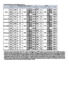
influential observations in binary logistic regression: An empirical study. Journal of Applied Statistics 2011;11:26-35. 6. Cook RD. Detection of influential observation in linear regression. Technometrics 1977;19:15-8.
7. Martín N, Pardo L. On the asymptotic distribution of Cook's distance in logistic regression models. Journal of Applied Statistics 2009;36:1119-46.
Cite this article as: Zhang Z. Residuals and regression diagnostics: focusing on logistic regression. Ann Transl Med 2016;4(10):195. doi: 10.21037/atm.2016.03.36
© Annals of Translational Medicine. All rights reserved.
atm.amegroups.com
Ann Transl Med 2016;4(10):195