ON THE MODELING OF MOTION IN WYNER-ZIV VIDEO CODING M

ON THE MODELING OF MOTION IN WYNER-ZIV VIDEO CODING M. Tagliasacchi, S. Tubaro, A. Sarti ∗ Dipartimento di Elettronica e Informazione Politecnico di Milano, Milan - Italy ABSTRACT Wyner-Ziv Encoder

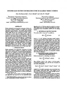
In the past few years, a number of practical video coding schemes following distributed source coding principles have emerged. One of the main goals of distributed video coding (DVC) is to enable a flexible distribution of the computational complexity between the encoder and the decoder, while approaching the coding efficiency of conventional closed-loop motion-compensated predictive codecs. In this paper we perform a rate-distortion analysis of a well-known Wyner-Ziv architecture, while focusing our attention on the impact of the motion modeling that is used for generating the side information at the decoder. Our analysis is structured according to a Kalman filtering problem and it allows us to compare three different scenarios: motion estimation at the encoder; motion interpolation at the decoder; and motion extrapolation at the decoder. 1. INTRODUCTION Distributed Video Coding (DVC) is a new video coding paradigm based on the principles of distributed source coding [1, 2]. DVC enables a flexible distribution of the computational complexity between the encoder and the decoder, together with an increased robustness against channel losses. In this paper we consider the WynerZiv codec that was first presented in [2] and further developed in [3], with the goal of evaluating the rate-distortion performance when different motion models are used. The work presented in this paper is partially inspired by [4]. The main differences lie in the fact that our analysis is based on a Kalman filtering approach. This choice allows us to decouple the noise term related to the natural evolution of scene motion, from the observation noise, which is introduced by motion estimation inaccuracy. In addition, we explicitly model the case that uses motion interpolation, and this is a widely adopted choice in the literature. 2. PDWZ VIDEO CODEC ARCHITECTURE The pixel domain Wyner-Ziv (PDWZ) video codec we refer to in this paper is based on the work in [2]. This coding architecture offers a pixel domain intra-frame encoder and inter-frame decoder with very low computational encoder complexity. The proposed encoding scheme is by far (several orders of magnitude) less complex then traditional video coding that performs motion estimation at the encoder. Figure 1 illustrates the global architecture of the PDWZ codec. Previously reconstructed frames are used at the decoder to generate the side information. In the literature we distinguish two cases: motion ˆ t−1 ) and the next (X ˆ t+1 ) frame interpolation, when the previous (X ∗ Distributed Source Coding Project, funded by the Italian Ministry of Education, University and Research

Wyner-Ziv Decoder

Slepian-Wolf Encoder

X

Uniform Quantizer

Bitplane 1 . . .

Bitplane N

Turbo Encoder .

Buffer

Slepian-Wolf Decoder Turbo Decoder

Wyner-Ziv Bitstream

Reconstruction

Xˆ

Y Feedback Channel

previously decoded frames

...

Motion Interpolation/ Extrapolation

Fig. 1. Block diagram of the pixel domain Wyner-Ziv codec.

are used to synthesize the side information for Xt ; motion extrapˆ t−1 , X ˆ t−2 ) are used olation, when the the previous two frames (X instead. More complex algorithms can be used, which combine both motion interpolation and extrapolation, although our analysis will focus on these two cases only. Each pixel in the Wyner-Ziv frame is uniformly quantized. Bitplane extraction is performed from the entire image and then each bitplane is fed to a turbo encoder to generate a sequence of parity bits. At the decoder, the generated side information will be used by the turbo decoder and reconstruction modules. The decoder operates in a bitplane-by-bitplane basis and begins by decoding the most significant bitplane and it only proceeds to the next bitplane after each bitplane is successfully turbo-decoded (i.e. when most of the errors are corrected). 3. PROBLEM STATEMENT Today’s video coding architectures conforming to the Wyner-Ziv paradigm are unable to achieve the coding efficiency of conventional motion-compensated predictive codecs. The existing gap can be attributed to different reasons: 1. Lack of side information at the encoder: Let X and Y be two correlated random sequences. The problem here is to ˆ given a condecode X to its quantized reconstruction X, ˆ when the side straint on the distortion measure E[d(X, X)], information Y is available only at the decoder. Let us denote by RX|Y (D) the rate-distortion function for the case WZ when Y is also available at the encoder, and by RX|Y (D) the case when only the decoder has access to Y . The Wyner-Ziv WZ theorem states that, in general, RX|Y (D) ≥ RX|Y (D) but WZ RX|Y (D) = RX|Y (D) for Gaussian memoryless sources and MSE as distortion measure. Therefore, a coding effiWZ ciency loss ∆R1 = RX|Y (D) − RX|Y (D) is observed in

applications when the hypothesis of the Wyner-Ziv theorem are not satisfied. 2. Entropy coding losses: DVC coding schemes use channel coding tools to perform source coding. Since the practical channel codes used in the context of DVC (Turbo, LDPC, etc.) only approach the Shannon’s bound, a coding efficiency loss ∆R2 stems from this fact. 3. Motion model inaccuracy: While motion-compensated predictive codecs do their best in order to accurately model the motion at the encoder side, Wyner-Ziv video coders perform the same operation at the decoder. Therefore, the side information Y available at the encoder side, i.e. the best motion compensated prediction of the current frame, is not available at the decoder, where a worse version of Y , say Y˜ , can be generated by motion interpolation and/or extrapolation. This results in a coding efficiency loss ∆R3 . This paper will focus on the estimation of this term. 4. ANALYSIS OF RATE-DISTORTION PERFORMANCE Following the same steps as in [4], let X(t) denote the current frame ˆ and X(k), k ∈ D the previously-decoded frames in the frame buffer D. Let Yi (t) be the side information generated by the side information generator gi ˆ Yi (t) = gi (X(k), k ∈ D),

i = 1, 2 .

(1)

The residual frame is ei (t) = X(t) − Yi (t),

i = 1, 2 .

T

∆

1

] = Φss (ω)e 2 ω

T

2 ωσ∆

Φcc (ω) = Φss (ω)

1

T

2 ωσ∆

(7)

The rate saving over INTRA-frame coding is [5]: ∆R =

1 8π 2

Z

+π

Z

+π

log2 −π

−π

Φee (ω) dω . Φss (ω)

(8)

Hence, the difference between the two systems using two motion vectors M V1 and M V2 is ∆R1,2 = ∆R1 − ∆R2 1 = 8π 2 =

1 8π 2

Z

+π

−π

Z

+π

Z

+π

−π

Z

Φee,1 (ω) log2 dω Φee,2 (ω)

+π

log2 −π

−π

1 ω T ωσ 2 ∆1

1 − e2

1 ω T ωσ 2 ∆2

1 − e2

dω .

mx(t-1)

X(t-2)

X(t-1)

X(t)

X(t+1)

Fig. 2. Motion trajectory model.

5. MOTION MODELING Wyner-Ziv video codecs generate the side information at the decoder, using previously reconstructed frames. Two main approaches have been explored in the literature: • Motion interpolation: One every N frames (most often N = 2) is labeled as key frame and it is INTRA encoded. The resulting group of picture (GOP) structure is I − W Z − . . . − W Z − I. For each Wyner-Ziv frame, the side information is obtained by motion compensated interpolation of the previous and next key frame. • Motion extrapolation: Only the first frame is a key frame and is INTRA coded. The resulting GOP structure is I − W Z − W Z − . . .. The side information for Wyner-Ziv frame is estimated through the motion extrapolation of the previouslydecoded frames (both Wyner-Ziv and key frames).

m(t) = ρm(t − 1) + z(t) .

(6)

2 1 T Φee (ω) = 2 − 2e 2 ω ωσ∆ Φss (ω)

mx(t+1)

(5)

(3)

where ∆ = (∆x , ∆y ) is the motion vector error, i.e. the difference between the motion vector used and the true motion vector. Φee (ω) = 2Φss (ω) − 2Φss (ω)e 2 ω

mx(t)

(4)

The power spectrum of the residual frame can be expressed as

Φcs (ω) = Φss (ω)E[e−jω

x

In this paper we want to compare these two approaches with the conventional case where the encoder performs motion estimation. In order to be able to model both motion interpolation and motion extrapolation we drift apart from the work in [4], introducing our analysis based on Kalman filtering. We denote by m(t) = (mx (t), my (t)) the true motion that a pixel/block is subjected to. Due to its nature, the motion is timevarying. We assume here a simple auto-regressive model

(2)

Φee (ω) = Φss (ω) − 2Re{Φce (ω)} + Φcc (ω)

t

(9)

(10)

Unlike [4], where m(t − 1) is the motion associated to the same spatial location at time t − 1, here the autoregressive model is assumed to be valid throughout the motion trajectories. This means that m(t − 1) is the motion vector corresponding to the spatial location pointed by m(t). Figure 2 illustrates this fact by means of an example for the case where only one of the two motion vector components are considered. We assume that the two components of the noise term z are statistically independent, and each of them can be modeled as a zero mean white random process with the same variance σz2 = σz2x = σz2y . From equation (10), we can immediately derive that 2 2 2 σm = σm = σm = x y

σz2 . 1 − ρ2

(11)

2 Intuitively, σm is an indication of motion complexity, i.e. a high 2 value of σm suggests that large displacements are expected. On the other hand, ρ measures the temporal coherence of the motion model. A value of ρ close to one indicates that motion has approximately uniform velocity (no acceleration/deceleration), covered/uncovered areas and scene changes are negligible. In spite of ρ, we use an

2 Table 1. σm and cSN R (Frame size QCIF, Block size 8 × 8

Sequence

Foreman

Coast.

Carphone

Stefan

Table

Silent

2 σm cSN R(dB)

9.46 1.54

0.76 5.69

7.23 0.44

15.40 1.58

2.09 1.05

1.93 0.86

equivalent representation introduced in [4], the motion temporal correlation signal-to-noise ratio cSN R = 10 log10

2 σm 1 = 10 log10 . σz2 1 − ρ2

• Motion estimation (ME) at the encoder: The motion estimation algorithm has access to X(t) and X(t−1). The observed motion is n(t) = m(t) + w(t) . (13) The observed motion differs from the true motion m(t) only because of motion vector accuracy (we neglect errors due to quantization, reflections, illumination changes). If 1/M pixel accuracy is used, the noise term wx,y (t) can be assumed to be uniformly distributed between −1/2M and +1/2M . The 2 2 2 = 1/12M 2 = σw resulting variance is σw = σw y x • Motion interpolation (MI) at the decoder: We assume here a I − W Z − I GOP structure. The motion interpolation algorithm has access to X(t − 1) and X(t + 1). The estimated motion is therefore (14)

where w(t) is defined as above. • Motion extrapolation (MX) at the decoder: The motion extrapolation algorithm has access to X(t − 1) and X(t − 2). The estimated motion is therefore n(t) = m(t − 1) + w(t) ,

2 ˆ E[(m(t) − m(t|t)) ]= T

(15)

where w(t) is defined as above. It is possible to combine equation (10) with equations (13), (14) and (15), respectively, to write the problem in the canonical form prescribed by Kalman filtering m(t) = Fm(t − 1) + v1 (t)

(16)

n(t) = Hm(t) + v2 (t) .

(17)

Table 5 shows how the three aforementioned problems are mapped onto a set of state-observation equations together with the other quantities needed to solve the Kalman filtering problem. Going back to our original problem, we want to obtain an estiˆ ˆ mate m(t) = E[m(t)|n(t), n(t − 1), . . . , n(0)] = m(t|t) of m(t) given a noisy observation n(t). Kalman filter theory states that it is possible to relate the variance of the error on the state of the Kalman ˆ predictor (ν(t) = m(t) − m(t|t − 1)) at time t + 1 with that at time t via the RDE (Riccati Differential Equation) P (t + 1) = F P (t)F T + V1 − K(t)(HP (t)H T + V2 )K T , (18) where P (t) = E[ν(t)ν(t)T ] and the Kalman gain K(t) is defined as K(t) = (F P (t)H T + V12 )(HP (t)H T + V2 )−1 . The variance

(19) −1

T

= P (t) − P (t)H [HP (t)H + V2 ]

HP (t) .

Upon convergence, P (t) = P (t − 1) = P . Using this equation into (18) we obtain the ARE (Algebraic Riccati Equation) and we can solve for P . We set P f ilt = P − P H T [HP H T + V2 ]−1 HP .

 (12)

Table 1 gives an indication of the parameters for a set of real sequences [4]. In the following, we distinguish three cases:

n(t) = m(t) + m(t + 1) + w(t) ,

of the error on the state of the Kalman filter is related to the one of the Kalman predictor by

P f ilt =

2 σ∆ 0

0 2 σ∆

 ,

(20)

2 where σ∆ is used in equation (9) in order to evaluate the rate-distortion gain of a given motion modeling scheme.

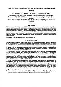
6. SIMULATION RESULTS In this section, we compare the rate-distortion performance of the three algorithms used to generate the side information: motion estimation (ME), motion interpolation (MI) and motion extrapolation (MX). As a benchmark, we consider a system that encodes the difference between Xt and Xt−1 , i.e. assuming zero motion. We dub this system FD, for frame difference. In this case, the expected variance 2 2 = σm . is σ∆ 2 for varFor each of the three cases, we numerically evaluate σ∆ 2 ious values of ρ and σm and we use equation (9) to assess the rate rebate with respect to the FD system. Figure 3 plots ∆R as a func2 tion of cSN R for different values of σm (from the rate-distortion theory we know that ∆P SN R ' 6∆R). We notice the same behavior in all cases. When we keep the 2 variance of the motion vectors σm fixed, increasing temporal coherence of motion (cSN R), we expect larger gains with respect to FD, that does not exploit motion at all. We can gain a further in2 sight comparing the plots in Figure 3 for the same value of σm . In fact, we notice that the maximum rate rebate is obtained for ME, 2 followed by MI and finally by MX. For example, setting σm = 1, ∆RM E/M I is as large as -0.8 bpp, while ∆RM I/M X is as large as -3.5 bpp. We notice that the gap between MI and ME gets narrower 2 increasing cSN R and decreasing σm . This is reasonable, since motion interpolation works well when the temporal coherence is high and displacements tend to be small. We have to point out that these figures refer to the encoding of a single Wyner-Ziv frame. In a complete video coding architecture, the total rate, including key frames, should be considered. While for ME and MX all frames (but the first one) take advantage of inter frame dependencies, for MI one every N frames (N = 2 in this case), is intra coded. Therefore, these results tend to overestimate the performance of motion interpolation. A fairer analysis should take into account the rate needed to encode key frames. The latter depends on the spatial power spectral density of the sequence (Φss (ω)), whereas our simplified analysis depends only on considerations based on motion. Table 3 compares the performance of practical algorithms used to generate the side information [4]. The behavior suggested by our analysis is confirmed by these figures. In fact, ME outperforms the other approaches for all of the tested sequences, followed by MI and MX in this order. The gain of ME over MI ranges between +0.44dB for Coastguard up to +2.08dB for Carphone. We notice that these two sequences are characterized by the highest and lowest temporal correlation (cSN R) respectively, validating the conclusions of our analysis.

ME mx,y (t + 1) = ρmx,y (t) + zx,y (t) nx,y (t) = mx,y (t) + wx,y (t) F = diag[ρ] H = diag[1] V1 = diag[σz2 ] 2 V2 = diag[σw ]

MI mx,y (t + 1) = ρmx,y (t) + zx,y (t) nx,y (t) = (1 + ρ)mx,y (t) + zx,y (t) + wx,y (t) F = diag[ρ] H = diag[1 + ρ] V1 = diag[σz2 ] 2 V2 = diag[σz2 + σw ], V12 = diag[σz2 ]

MX mx,y (t + 1) = ρmx,y (t) + zx,y (t) nx,y (t) = ρ1 mx,y (t) − ρ1 zx,y (t − 1) + wx,y (t) F = diag[ρ] H = diag[1/ρ] V1 = diag[σz2 ] 2 V2 = diag[(1/ρ2 )σz2 + σw ]

Table 2. Systems of equations corresponding to the three motion models: ME - Motion Estimation, MX - Motion Extrapolation, MI - Motion Interpolation.

σ2 = 3 m σ2m σ2 m

−4 −5 −6

=5 = 10

−7

−1

−1

−2

−2

−3

−3

, bits/pixel

2

σm = 2

0

−4 −5

MX,FD

2

0

−6

ΔR

−2

σm = 1 Δ RMI,FD, bits/pixel

ΔR

−1

σ2m = 0.5

−3

ME,FD

, bits/pixel

0

−7

−4 −5 −6 −7

−8

−8

−8

−9

−9

−9

−10

0

2

4 6 cSNR (dB)

8

−10

10

0

2

4 6 cSNR (dB)

8

10

−10

0

2

4 6 cSNR (dB)

8

10

Fig. 3. Comparison of the rate-distortion performance between motion estimation (ME), motion interpolation (MI) and motion extrapolation (MX). The rate rebate with respect to simple frame differencing (FD) is shown

Table 3. Comparison of different algorithms used to generate the side information (in dB) Sequence

Foreman

Coast.

Carphone

Stefan

Table

FD MX MI ME

28.17 30.66 32.56 33.21 +5.04 +2.55 +0.65

27.32 30.82 32.17 32.61 +4.29 +1.79 +0.44

29.77 29.03 31.72 33.80 +4.03 +4.77 +2.08

19.48 22.88 23.54 24.84 +5.36 +1.96 +1.30

27.10 30.48 32.20 33.86 +6.76 +3.38 +1.66

ME − F D ME − MX ME − MI

Silent

fact, they do not apply to other distributed source coding based coding schemes such as PRISM [1], where the decoder is able to build a motion model comparable to the one that can be obtained by performing motion estimation at the encoder.

32.43 33.62 8. REFERENCES 36.09 38.11 [1] Rohit Puri and Kannan Ramchandran, “PRISM: A New Robust Video Coding Architecture based on Distributed Compression Principles,” +5.68 in Allerton Conference on Communication, Control and Computing, +4.49 Urbana-Champaign, IL, October 2002. +2.02

7. CONCLUSIONS In this paper we analyze the coding efficiency of a Wyner-Ziv coding architecture, with respect to conventional schemes that perform motion estimation at the encoder. Unlike similar approaches recently appeared in the literature, our analysis builds upon Kalman filtering in order to explicitly model the case that performs motion compensated interpolation at the decoder. The results of the analysis are validated by experimental results on real test sequences. Our current activities focus on studying the rate-distortion performance of other motion modeling schemes adopted in the literature such as mixed motion extrapolation/interpolation [6], motion interpolation with longer GOP size and motion extrapolation using hash functions [7]. We need to emphasize that the results presented in this paper are valid for the coding architecture summarized in Section 2. In

[2] Anne Aaron, Rui Zhang, and Bernd Girod, “Wyner-Ziv coding of motion video,” in Proceedings of the 36th Asilomar Conference on Signals, Systems, and Computers, Pacific Grove, CA, October 2002, vol. 1, pp. 240–244. [3] Bernd Girod, Anne Aaron, Shantanu Rane, and David Rebollo Monedero, “Distributed video coding,” Proceedings of the IEEE, vol. 93, pp. 71–83, January 2005. [4] Li Zhen and E. J. Delp, “Wyner-Ziv video side estimator: Conventional motion search methods revisited,” in Proceedings of the International Conference on Image Processing, Genova, Italy, September 2005, pp. 825 – 828. [5] T. Berger, Rate Distortion Theory, Prentice Hall, 1971. [6] Lu´ıs Nat´ario, Catarina Brites, Jo˜ao Ascenso, and Fernando Pereira, “Extrapolating side-information for low-delay pixel-domain distributed video coding,” in Internationa Workshop on Very Low Bitrate Video Coding, Costa del Rei, Sardinia, Italy, September 2005. [7] Anne Aaron and Bernd Girod, “Wyner-ziv video coding with lowencoder complexity,” in Picture Coding Symposium, San Francisco, CA, December 2004.