On the multiple unicast capacity of 3-source, 3-terminal directed ...

On the multiple unicast capacity of 3-source, 3-terminal directed acyclic networks Shurui Huang, Student Member, IEEE and Aditya Ramamoorthy, Member, IEEE Department of Electrical and Computer Engineering Iowa State University, Ames, Iowa 50011 Email: {hshurui, adityar}@iastate.edu

Abstract—We consider a directed acyclic network with unitcapacity edges and n source-terminal(si − ti ) pairs that wish to communicate at unit rate via network coding. The connectivity between the si − ti pairs is quantified by means of a connectivity level vector, [k1 k2 . . . kn ] such that there exist ki edge-disjoint paths between si and ti . In this work we attempt to classify networks based on the connectivity level. Specifically, for case of n = 3, and a given connectivity level vector [k1 k2 k3 ], we aim to either present a constructive network coding scheme or an instance of a network that cannot support the desired rate. Certain generalizations for the case of higher n have also been found.

I. I NTRODUCTION In a network that supports multiple unicast, there are several source terminal pairs; each source wishes to communicate with its corresponding terminal. Multiple unicast connections form bulk of the traffic over both wired and wireless networks. Thus, network coding schemes that can help improve network throughput for multiple unicasts are of considerable interest. However, it is well recognized that the design of constructive network coding schemes for multiple unicasts is a hard problem. Specifically, it is known that there are instances of networks where linear (whether scalar or vector) network coding is insufficient [1]. The multiple unicast problem has been examined for both directed acyclic networks [2][3][4] and undirected networks [5] in previous work. The work of [6], provides an information theoretic characterization for directed acyclic networks. However, this bound is not computable as there is no upper bound on the cardinality of the random variables involved in the characterization. There have been attempts to find constructive solutions by leveraging linear network coding between pairs of flows (much like the butterfly structure). The work of [7] suggests back pressure algorithms for finding achievable rates using XOR operation between pairs of flows, while the work of [2] attempts to address it by packing butterfly networks within the original graph. The work of [3] (also see [8]), considers the multiple unicast problem in the case of two sourceterminal pairs where each terminal wants to operate at unitrate. Specifically, [3] presents a graph-theoretic condition that can be efficiently verified for checking the existence of a network coding solution for the unit-rate problem. The work This research was supported in part by NSF grant CCF-1018148.

of [9], also considers schemes for two-unicast, where one can trade-off rates between the different connections. For the case of two-unicast, [10] and [11] propose outer bounds on the capacity region. The work of Das et al. [12], [13] considers multiple unicast for three source-terminal pairs using the idea of interference alignment that was proposed in the area of physical layer wireless communication [14]. This can be viewed as a scheme where the network operates via random linear network coding and the sources choose appropriate precoding matrices in order to satisfy the demands of each terminal. This is a potentially powerful technique that allows us to achieve half of the minimum cut of each source-terminal pair simultaneously. However, the scheme of [12], [13] requires several algebraic conditions to be satisfied in order for the technique to be applicable1 and it is unclear whether this can be done efficiently. Some progress on this issue has been reported in [15]. In this work we consider linear network coding schemes for wired three-source, three-terminal directed acyclic networks with unit capacity edges. There are source-terminal pairs denoted si −ti , i = 1, . . . , 3, such that the maximum flow from si to ti is ki . Each source contains a unit-entropy message that needs to be communicated to the corresponding terminal. In general, this is a hard problem as bounds or constructive schemes may depend heavily on the network topology. In this work, for a given connectivity level vector [k1 k2 k3 ] we attempt to either design a constructive scheme based on linear network codes or demonstrate an instance of a network where supporting unit-rate transmission is impossible. Our achievability schemes use a combination of random linear network coding and appropriate precoding. However, unlike [12], our schemes are not asymptotic. In particular, our solutions are based either scalar codes or vector codes that operate over two time units (i.e., two network uses). This is potentially useful, as one could arrive at multiple unicast schemes for arbitrary rates by packing unit-rate structures for which our achievability schemes apply. A. Main Contributions • For the case of three unicast sessions, we identify certain feasible and infeasible connectivity levels [k1 k2 k3 ]. For the 1 In the wireless physical layer setting, these can be assumed to hold under appropriate channel models.

is downstream of another node j (or edge ej ) if there exists a path from j (or ej ) to i (or ei ). Vector linear network coding is a generalization of the scalar case, where we code across the source symbols in time, and the intermediate nodes can implement more powerful operations. Formally, suppose that the network is used over T time units. We treat this case as follows. Source node si now observes (1) (T ) Owing to space limitations, proofs of several results are not a vector source [Xi . . . Xi ]. Each edge in the original provided. These can be found in the full version of the paper graph is replaced by T parallel edges. In this graph, suppose that is available at [16]. This paper is organized as follows. In that a node j has a set of βinc incoming edges over which Section II, we introduce the network coding model and prob- it receives a certain number of symbols, and βout outgoing lem formulation. Section III discusses infeasible instances, and edges. Under vector network coding, j chooses a matrix of Section IV discusses our achievable schemes for 3-source, 3- dimension βout × βinc . Each row of this matrix corresponds terminal multiple unicast networks. Section V concludes the to the local coding vector of an outgoing edge from j. Note that the general multiple unicast problem, where paper with a discussion of future work. edges have different capacities and the sources have different entropies can be cast in the above framework by splitting II. P RELIMINARIES higher capacity edges into parallel unit capacity edges, a We represent the network as a directed acyclic graph G = higher entropy source into multiple, collocated unit-entropy (V, E). Each edge e ∈ E has unit capacity and can transmit sources; and the corresponding terminal node into multiple, one symbol from a finite field of size q per unit time (we are collocated terminal nodes. free to choose q large enough). If a given edge has higher An instance of the multiple unicast problem is specified by capacity, it can be treated as multiple unit capacity edges. A the graph G and the source terminal pairs si −ti , i = 1, . . . , n, directed edge e between nodes i and j is represented as (i, j), and is denoted < G, {si − ti }n1 , {Ri }n1 >, where the rate Ri so that head(e) = j and tail(e) = i. A path between two denotes the entropy of the ith source. The si − ti connections nodes i and j is a sequence of edges {e1 , e2 , . . . , ek } such that will be referred to as sessions that we need to support. tail(e1 ) = i, head(ek ) = j and head(ei ) = tail(ei+1 ), i = The instance is said to have a scalar linear network coding 1, . . . , k − 1. The network contains a set of n source nodes solution if there exist a set of linear encoding coefficients for si and n terminal nodes ti , i = 1, . . . n. Each source node si each node in V such that each terminal ti can recover Xi observes a discrete integer-entropy source, that needs to be using the received symbols at its input edges. Likewise, it communicated to terminal ti . Without loss of generality, we is said to have a vector linear network coding solution with assume that the source (terminal) nodes do not have incoming vector length T if the network employs vector linear network (1) (T ) (outgoing) edges. codes and each terminal ti can recover [Xi . . . Xi ]. If We now discuss the network coding model under con- the instance has either a scalar or a vector network coding sideration in this paper. For the sake of simplicity, suppose solution, we say that it is feasible. that each source has unit-entropy, denoted by Xi . In scalar In a routing solution, each edge carries a copy of one of linear network coding, the signal on an edge (i, j), is a linear the sources, i.e., each coding vector is such that at most one combination of the signals on the incoming edges on i or entry takes the value 1, all others are 0. Scalar (vector) routing the source signals at i (if i is a source). We shall only be solutions can be defined in a manner similar to scalar (vector) concerned with networks that are directed acyclic and can network codes. We now define some quantities that shall be therefore be treated as delay-free networks [17]. Let Yei (such used throughout the paper. that tail(ei ) = k and head(ei ) = l) denote the signal on edge Definition 2.1: Connectivity level. The connectivity level ei ∈ E. Then, we have for source-terminal pair si − ti is said to be n if the maximum ∑ flow between si and ti in G is n. The connectivity level Yei = fj,i Yej if k ∈ V \{s1 , . . . , sn }, and of the set of connections s1 − t1 , . . . , sn − tn is the vector {ej |head(ej )=k} [max-flow(s1 −t1 ) max-flow(s2 −t2 ) . . . max-flow(sn −tn )]. n ∑ We conclude this section by observing that a multiple Yei = aj,i Xj where aj,i = 0 if Xj is not observed at k. unicast instance G with n (si −ti ) pairs and connectivity level j=1 [n n . . . n] is always feasible. Specifically, we employ vector (1) (n) The coefficients aj,i and fj,i are from the operational field. routing over n time units. Source si observes [Xi . . . Xi ] Note that since the graph is directed acyclic, it is equivalently symbols. Each edge e in the original graph G is replaced by n 1 2 n possible to express ∑nYei for an edge ei in terms of the sources parallel edges, e , e , . . . , e . Let Gα represent the subgraph of this graph consisting of edges with superscript α. It is Xj ’s. If Yei = k=1 βei ,k Xk then we say that the global coding vector of edge ei is β ei = [βei ,1 · · · βei ,n ]. We shall evident that max-flow(sα −tα ) = n over Gα . Thus, we transmit (1) (n) also occasionally use the term coding vector instead of global Xα , . . . , Xα over Gα using routing, for all α = 1, . . . , n. coding vector in this paper. We say that a node i (or edge ei ) demands of all the terminals. In general, though a network feasible cases, we provide efficient schemes based on linear network coding. For the infeasible cases, we provide counterexamples, i.e., instances of graphs where the multiple unicast cannot be supported under any (potentially nonlinear) network coding scheme. • We identify certain infeasible instances for two unicast sessions, where the source rates are not necessarily the same.

with the above connectivity level may not be able to support a scalar routing solution; an instance is shown in [18]. III. N ETWORK CODING FOR THREE UNICAST SESSIONS I NFEASIBLE I NSTANCES It is clear based on the discussion above that for three unicast sessions if the connectivity level is [3 3 3], then a vector routing solution always exists. We investigate counterexamples for certain connectivity levels in this section. This material has appeared in a previous paper by the authors and we only state the results here and refer the reader to [18] for details. Lemma 3.1: [18] There exist multiple unicast instances with three unicast sessions, < G, {si −ti }3i=1 , {1, 1, 1} > such that the connectivity levels [1 1 3], [2 2 2] and [2 2 3] are infeasible. The [2 3] counter-example in [18] can be generalized to an instance with two unicast sessions with connectivity level [n1 n2 ] that cannot support rates R1 = n1 , R2 = n2 −3n1 /2+ 1 when n2 ≥ 3n1 /2 and n1 > 1. Theorem 3.2: For a directed acyclic graph G with two s−t pairs, if the connectivity level for (s1 , t1 ) is n1 , for (s2 , t2 ) is n2 , where n2 ≥ 3n1 /2 and n1 > 1, there exist instances that cannot support R1 = n1 and R2 = n2 − 3n1 /2 + 1. Proof: Omitted owing to space limitations. IV. N ETWORK CODING FOR THREE UNICAST SESSIONS F EASIBLE I NSTANCES In the discussion below, we show that all the instances with the connectivity levels [1 3 3], [2 2 4] and [1 2 5] are feasible using linear network codes. As pointed out by the work of [17], under linear network coding, the case of multiple unicast requires (a) the transfer matrix for each source-terminal pair to have a rank that is high enough, and (b) the interference at each terminal to be zero. Under random linear network coding, it is possible to assert that the rank of any given transfer matrix from a source si to a terminal tj has w.h.p. a rank equal to the minimum cut between si and tj ; this in general is problematic for satisfying the zero-interference condition. Our strategies rely on a combination of graph-theoretic and algebraic methods. Specifically, starting with the connectivity level of the graph, we use graph theoretic ideas to argue that the transfer matrices of the different terminals have certain relationships. The identified relationships then allow us to assert that suitable precoding matrices that allow each terminal to be satisfied can be found. We begin with the following definitions. Definition 4.1: Minimality. Consider a multiple unicast instance < G = (V, E), {si − ti }n1 >, with connectivity level [k1 k2 . . . kn ]. The graph G is said to be minimal if the removal of any edge from E reduces the connectivity level. If G is minimal, we will also refer to the multiple unicast instance as minimal. Clearly, given a non-minimal instance G = (V, E), we can always remove the non-essential edges from it to obtain the minimal graph Gmin ; this does not affect feasibility.

Definition 4.2: Overlap edge. An edge e is said to be an overlap edge for paths Pi and Pj in G, if e ∈ Pi ∩ Pj . Definition 4.3: Overlap segment. Consider a set of edges Eos = {e1 , . . . , el } ⊂ E that forms a path. This path is called an overlap segment for paths Pi and Pj if (i) ∀k ∈ {1, . . . , l}, ek is an overlap edge for Pi and Pj , (ii) none of the incoming edges into tail(e1 ) are overlap edges for Pi and Pj , and (iii) none of the outgoing edges leaving head(el ) are overlap edges for Pi and Pj . Our solution strategy is as follows. We first convert the original instance into another structured instance where each internal node has at most degree three (in-degree + out-degree). We then convert this new instance into a minimal one, and develop the code assignment algorithm. It will be evident that using this network code, one can obtain a network code for the original instance. Following [19] we can efficiently construct a structured ˆ = (Vˆ , E) ˆ in which each internal node v ∈ Vˆ is graph G of total degree at most three with the following properties. ˆ is acyclic. (a) G (b) For every source (terminal) in G there is a corresponding ˆ source (terminal) in G. (c) For any two edge disjoint paths Pi and Pj for one unicast ˆ session in G, there exist two vertex disjoint paths in G ˆ for the corresponding session in G. ˆ can be efficiently (d) A feasible network coding solution in G turned into a feasible network coding solution in G. In all the discussions below, we will assume that the graph G is structured. It is clear that this is w.l.o.g. based on the previous arguments. We state the result for connectivity level [1 3 3] here and refer the interested reader to the proof in [18]. Theorem 4.4: [18] A multiple unicast instance with three sessions, < G, {si − ti }31 , {1, 1, 1} > with connectivity level at least [1 3 3] is feasible. A. Code Assignment Procedure For Instances With Connectivity Level [2 2 4] We first investigate a two-unicast scenario with connectivity level [2 4] and rate requirement {2, 1} and use that in conjunction with vector network coding to address three-unicast with connectivity level [2 2 4]. We use random linear coding and precoding at the sources to arrive at the result. Proving the existence of an appropriate precoding scheme requires us to explore the relation between the structure of the graph and the properties of the transfer matrices. Lemma 4.5: A minimal multiple unicast instance < G, {s1 − t1 , s2 − t2 }, {2, 1} > with connectivity level [2 4] is feasible. Proof: Let P1 = {P11 , P12 } denote two edge disjoint paths (also vertex disjoint due to the structured nature of G) from s1 to t1 and P2 = {P21 , P22 , P23 , P24 } denote the four vertex disjoint paths from s2 to t2 . Let the source messages at s1 be denoted by X1 and X2 , and the source message at s2

s2

s1

P11 P12 P21 P22 P23

Eb

P24

Eos3 Eos4

Er (Eos1)

t2

t1

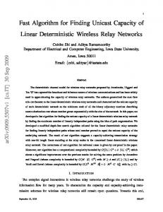
Fig. 1. A network with connectivity levels [2 4] and rate {2, 1}. A linear network coding solution can be found .

by X3 . We color the edges of the graph such that each edge on P11 is colored red, each edge on P12 is colored blue and each edge on a path in P2 is colored black. As the paths in P1 and P2 are vertex-disjoint, it is clear that a node with an in-degree of two is such that its outgoing edge has two colors (either (blue, black) or (red, black)). The path further downstream continues to have two colors until it reaches a node of out-degree two. Such an overlap segment with two colors will be referred to as a mixed color overlap segment. We shall also use the terms red or blue overlap segment to refer to segments with colors (red, black) and (blue, black) respectively. Note that by our naming convention path Pij is a path that enters terminal ti . Under the topological order in G we can identify the overlap segment on Pij that is closest to ti . In the discussion below this will be referred to as the last overlap segment with respect to path Pij . Two overlap segments Eos1 and Eos2 are said to be neighboring with respect to Pij if there are no overlap segments between them along Pij . Claim 4.6: Consider two neighboring mixed color overlap segments Eos1 and Eos2 with respect to path P1i ∈ P1 . Then Eos1 and Eos2 cannot lie on the same path P2j ∈ P2 . proof : This follows from the minimality of graph. Likewise, two neighboring mixed color overlap segments Eos1 and Eos2 with respect to P2i , cannot lie on the same path P1j . To explain our coding scheme, we first denote the last red (blue) overlap segment with respect to P11 (P12 ) by Er (Eb ). If there is no Er , then X1 can be transmitted along P11 . According to Lemma A.2, X2 and X3 can be transmitted to t1 and t2 respectively. A similar argument can be applied to the case when there is no Eb . Hence we assume that both Er and Eb exist. Based on their locations in G, we distinguish the following two cases. • Case 1: Er and Eb are on different paths ∈ P2 . W.l.o.g. we assume that Er and Eb are on paths P21 and P22 . If there are no mixed color overlap segments on either P23 or P24 , X3 can be transmitted to t2 through the overlap segment free path, and X1 , X2 can be routed to t1 . Therefore, we

focus on the case that there are mixed color overlap segments on both P23 and P24 . Let Eosi denote the last mixed color overlap segments with respect to P2i , i = 1, . . . , 4 (see example in Fig. 1). Our coding scheme is as follows. Symbol Xi is transmitted over the outgoing edge from s1 over P1i , i = 1, 2; symbols θj X3 are transmitted over the outgoing edges of s2 over P2j , j = 1, . . . , 4 respectively. The values of θj ∈ GF (q) will be chosen as part of the code assignment below. Let the coding vectors at each intermediate node be specified by indeterminates for now. The overall transfer matrix from the pair of sources {s1 , s2 } to t1 can be expressed as [ ] α1 β1 γ11 γ12 γ13 γ14 [M11 | M12 ] = , α2 β2 γ21 γ22 γ23 γ24 where M11 is a 2 × 2 matrix which contains the coefficients for X1 and X2 and M12 is a 2 × 4 matrix which contains the coefficients for θi X3 , i = 1, . . . , 4, i.e., the received vector at t1 is [M11 | M12 ][X1 X2 | θ1 X3 . . . θ4 X3 ]T . Recall that Er and Eb are the last mixed color overlap segments with respect to P11 and P12 . Thus, they carry the same information as the incoming edges of t1 which implies that the row vectors of [M11 | M12 ] are the coding vectors on Er and Eb respectively. Similarly, the transfer matrix from {s1 , s2 } to the edge set {Er , Eb , Eos3 , Eos4 } can be expressed as   α1 β1 γ11 γ12 γ13 γ14  α2 β2 γ21 γ22 γ23 γ24   [M21 | M22 ] =   α3 β3 γ31 γ32 γ33 γ34  . α4 β4 γ41 γ42 γ43 γ44 Note that the entries of the transfer matrices above are functions of the choice of local coding vectors in the network. As there exist two edge disjoint paths from s1 to {Er , Eb }, the determinant of M11 is not identically zero. Similarly, since the edges Er , Eb , Eos3 and Eos4 lie on different paths in P2 , there are four edge disjoint paths from s2 to {Er , Eb , Eos3 , Eos4 }, and the determinant of M22 is not identically zero. This implies that their product is not identically zero. Hence, by the Schwartz-Zippel lemma, under random linear coding there exists an assignment of local coding vectors so that rank(M11 ) = 2 and rank(M22 ) = 4. We assume that the local coding vectors are chosen from a large enough field GF (q) so that this is the case. For this choice of local coding vectors we propose a choice of θ = [θ1 θ2 θ3 θ4 ]T such that the decoding is simultaneously successful at both t1 and t2 . Decoding at t1 : As M11 is a square full-rank matrix, we only need to null the interference from s2 . Accordingly, we choose θ from the null space of M12 , i.e., M12 θ = 0.

(1)

There are at least q 2 − 1 such non-zero choices for θ as M12 is a 2 × 4 matrix. Decoding at t2 : The primary issue is that one needs to demonstrate that the choice of θ allows both terminals to

simultaneously decode. Indeed, it may be possible that our choice of θ along with a specific network topology may make it impossible to decode at t2 . The key argument that this does not happen requires us to leverage certain topological properties of the overlap segments, that we present below. Claim 4.7:In G either one or both of the following statements hold. (i) Er is the last overlap segment w.r.t. P21 . (ii) Eb is the last overlap segment w.r.t. P22 . Proof: Assume that neither statement is true. This means that there is a blue overlap segment Eb′ below Er along P21 , and there is a red overlap segment Er′ below Eb along P22 . Thus, Er′ is upstream of Er and Eb′ is upstream of Eb . However, this means that edges Er′ , Er , Eb′ and Eb form a cycle, which is a contradiction. In the discussion below, w.l.o.g., we assume that Er is the last overlap segment on P21 . The argument above allows us to identify three edges, Er , Eos3 and Eos4 that carry the same symbols as those entering t2 . Our main idea is to cancel the X1 and X2 component using the information on Eos3 and Eos4 while retaining the X3 component. Let γ i represent the vector [γi1 γi2 γi3 γi4 ]T , i = 1, . . . , 4 in the discussion below. Note that if [α3 β3 ] and [α4 β4 ] are linearly independent, there exist δ3 and δ4 such that [α1 β1 ] = δ3 [α3 β3 ] + δ4 [α4 β4 ], where δ3 and δ4 are not both zero. Thus, t2 can recover [−γ 1 + δ3 γ 3 + δ4 γ 4 ]T θX3 . Note that γ T1 θ = 0, by the constraint on θ above, thus we only need to pick θ such that [δ3 γ 3 + δ4 γ 4 ]T θ ̸= 0. To see that this can be done, we note that M22 is full rank which implies that the matrix [γ 1 γ 2 (δ3 γ 3 +δ4 γ 4 )]T is full rank. Therefore, there exist at most q choices for θ such that [γ 1 γ 2 (δ3 γ 3 +δ4 γ 4 )]T θ = 0. Hence, there are at least q 2 − q − 1 > 0 non-zero choices for θ that allow decoding at t1 and t2 simultaneously. If [α3 β3 ] and [α4 β4 ] are dependent, decoding can be performed simply by working only with the received values over Eos3 and Eos4 using a similar argument as above. • Case 2: Er and Eb are on the same path P2i . We proceed by identifying the blue overlap segment Eb′ that is a neighbor of Eb w.r.t. P12 and adapting the analysis above. The details can be found in [16]. By using the result of Lemma 4.5 and vector network coding over two time units, we have the following theorem when the connectivity level is [2 2 4]. Theorem 4.8: A multiple unicast instance with three sessions, < G, {si − ti }31 , {1, 1, 1} > with connectivity level at least [2 2 4] is feasible. B. Code Assignment Procedure For Instances With Connectivity Level [1 2 5] We now consider the network code assignment for networks where the connectivity level is [1 2 5]. The code assignment in this case requires somewhat different techniques. In particular, the idea of using a two-session unicast result along with vector network coding does not work unlike the cases

considered previously. At the top level, we still use random network coding followed by appropriate precoding to align the interference seen by the terminals. However, as we shall see below, we will need to depart from a purely random linear code in the network in certain situations. As before, we consider a minimal structured graph G and let Xi be the source symbol at source node si for i = 1, . . . , 3 and P1 = {P11 } denote the path from s1 to t1 , P2 = {P21 , P22 } denote the edge disjoint paths from s2 to t2 , P3 = {P31 , P32 , P33 , P34 , P35 } denote the edge disjoint paths from s3 to t3 . Our scheme operates as follows: X1 is transmitted over the outgoing edge from s1 along P11 , ξi X2 are transmitted over the outgoing edges of s2 along P2i , i = 1, 2, and θj X3 are transmitted over the outgoing edges of s3 along P3j , j = 1, . . . , 5 where ξ = [ξ1 ξ2 ]T and θ = [θ1 . . . θ5 ]T are precoding vectors chosen from a finite field with size q. Let Mi denote the transfer matrix from {s1 , s2 , s3 } to terminal ti . The matrix Mi is partitioned into blocks so that Mi = [Mi1 | Mi2 | Mi3 ], and each Mij corresponds to the transformation from source sj to terminal ti , i.e., the number of columns in Mij is 1, 2 and 5 for j = 1, 2 and 3 respectively. Similarly, the number of rows in Mij is 1, 2 and 5 for i = 1, 2 and 3 respectively. In the discussion below we will need to refer to the individual entries of M1 and M2 . Accordingly, we express these matrices explicitly as follows. [ ] M1 = [M11 | M12 | M13 ] = α1 | β T | γ T = [α1 | β1 β2 | γ1 γ2 γ3 γ4 γ5 ] , [ ] T T α1′ β ′ 1 γ ′ 1 M2 = [M21 | M22 | M23 ] = T T α2′ β ′ 2 γ ′ 2 ] [ ′ ′ ′ ′ ′ ′ ′ ′ γ15 γ14 γ13 β12 γ12 α1 β11 γ11 . = ′ ′ ′ ′ ′ ′ ′ α2′ β21 γ25 γ24 γ23 β22 γ22 γ21 We are given that min−cut(s1 −t1 ) = 1, min−cut(s2 −t2 ) = 2 and min − cut(s3 − t3 ) = 5. This implies that det(Mii ) is not identically zero for i = 1, . . . , 3, and furthermore that their product det(M11 ) det(M22 ) det(M33 ) is not identically zero. We first identify a minimal structured subgraph G′ of G that has the following properties. ′ (i) There exists a path P11 , from s1 to t1 , ′ ′ from s2 to t2 , and P22 (ii) vertex disjoint paths P21 ′ (iii) path P1→2 from s1 to t2 and ′ (iv) path P2→1 from s2 to t1 . Here again, G′ is said to be minimal if the removal of any edge from it causes one of the above properties to fail. We note that it is possible that there do not exist any paths from s1 to t2 or from s2 to t1 in G. These situations are considered below. Our analysis depends on the following topological properties of G′ . Case 1: The graph G′ is such that ′ ′ • there is no path from s1 to t2 in G , i.e., P1→2 = ∅ (this happens only if there is no path from s1 to t2 in G), or

′ there is no path from s2 to t1 in G′ , i.e., P2→1 = ∅ (this happens only if there is no path from s2 to t1 in G), or ′ ′ ′ • there are paths P1→2 and P2→1 in G , and there are ′ ′ ′ overlap segments between P11 and P21 ∪ P22 . ′ Case 2: The graph G is such that ′ ′ ′ ′ • there are paths P1→2 and P2→1 in G , and P11 does not ′ ′ overlap with either P21 or P22 . We emphasize that the condition of Case 2 is the logical negation of the conditions in Case 1. Theorem 4.9: A multiple unicast instance with three sessions, < G, {si − ti }31 , {1, 1, 1} >, with connectivity level [1 2 5] is feasible. •

G’

G’ s1

s2

P’11

P’21

t1

s2

s1 P’22

P’11

t2

P’21

t1

P’22

We begin by noting that since rank(M22 ) = 2, M22 ξ ̸= 0, as long as ξ ̸= 0. Next, we argue according to the topological structure of G′ . The following possibilities can occur. ′ (i) There is no path from s1 to t2 in G′ , i.e., P1→2 = ∅. This ′ ′ implies that α1 = α2 = 0 and in G, interference at t2 only exists due to s3 . Next, at least one component of M22 ξ will be non-zero, based on the argument above; w.l.o.g. assume that it is the first component. We choose θ to satisfy γ′1 θ = 0 T

(4)

It is evident that there are at least q 3 − 1 non-zero choices of θ that satisfy the required constraints on θ (eqs. (3) and (4)). Hence t2 can decode. ′ ′ (ii) There exists a path P1→2 from s1 to t2 , i.e., P1→2 ̸= ∅.. This means that M21 is not identically zero. Here, we first align the interference from s3 within the span of interference from s1 by selecting an appropriate θ. We have the following lemma. Lemma 4.10:If M21 ̸= 0, there exist at least q 4 − 1 choices for θ such that M23 θ = cM21 (5) where c is some constant. Proof: First, w.l.o.g., we assume α2′ ̸= 0. Hence, there exists a full rank 2 × 2 upper triangular matrix U such that U M21 = [0 α2′ ]T . Next, define

t2

′

(a)

[1 0]U M23 = γ e1T

(b)

′ overlaps with P ′ . (b) Subgraph G′ Fig. 2. (a) Subgraph G′ when P11 21 ′ overlaps with both P ′ and P ′ . when P11 21 22

Proof: We break up the proof into two parts based on type of the subgraph G′ that we can find in G. Proof when there exists a subgraph G′ that satisfies the conditions of Case 1: We perform random linear coding over the graph G over a large enough field. In the discussion below, we will leverage the fact that multivariate polynomials that are not identically zero, evaluate to a non-zero value with high probability (w.h.p.) under a uniformly random choice of the variables. This is needed at several places. By using standard union bound techniques, we can claim that our strategy works with high probability. In particular, in the discussion below, we assume that the matrices Mii , i = 1, . . . , 3 are full rank and design appropriate precoding vectors ξ and θ. Decoding at t1 : For t1 to decode X1 , we need to have, α1 ̸= 0 and the precoding constraints. [β1 β2 ]ξ = 0

(2)

[γ1 γ2 γ3 γ4 γ5 ]θ = 0

(3)

There are at least q − 1 non-zero vectors ξ and q 4 − 1 nonzero vectors θ that can be selected from the field of size q such that eq. (2) and eq. (3) are satisfied. Decoding at t2 :

′

(6) ′

and choose θ to satisfy γ e1T θ = 0 and set c = γ 2T θ/α2′ . Upon inspection, it can be verified that this implies that U M23 θ = cU M21 . As U is invertible, and there is only one linear constraint on θ, we have the required conclusion. Thus, under this choice of θ, the interference from s3 is aligned within the span of the interference from s1 at t2 . Let X = [X1 X2 X3 ]T . The received signal at t2 is given by [ ] X1 + cX3 [M21 | M22 ξ | M23 θ]X = [M21 M22 ξ] (7) X2 To conclude the decoding argument for t2 , we need the claim below. Claim 4.11:If M21 is not identically zero, under random linear coding w.h.p., there exists a ξ such that rank[M21 M22 ξ] = 2 and [β1 β2 ]ξ = 0. Proof: We will show that there exists an assignment of local coding vectors such that det[M21 M22 ξ] ̸= 0. This will imply that w.h.p. under random linear coding, this property continues to hold. ′ Suppose that there is no path from s2 to t1 in G, i.e., P2→1 = ∅ and [β1 β2 ] is identically zero. This does not impose any constraint on ξ. Next, M22 is full rank w.h.p. Hence, we can choose a ξ such that required condition is satisfied. ′ If there exists a path P2→1 from s2 to t1 in G′ , [β1 β2 ] is not identically zero. W.l.o.g., we assume that β1 is not identically zero. By Lemma A.3, proving that det[M21 M22 ξ] ̸= 0, is equivalent to checking that the determinant in (11) is not

identically zero. Now we demonstrate that there exists a set of local coding vectors such that the determinant in (11) is ′ ′ ′ non-zero. We consider the subgraph G′ = P11 ∪ P21 ∪ P22 ∪ ′ ′ P1→2 ∪ P2→1 (identified above) - our choice of the coding vectors on all the other edges will be assigned to the zero ′ ′ vector. As both P1→2 ̸= ∅ and P2→1 ̸= ∅, we only consider ′ ′ ′ the case where P11 overlaps with P21 ∪ P22 . We distinguish the following cases. ′ ′ ′ 1) P11 overlaps with either P21 or P22 . W.l.o.g., assume ′ ′ ′ it is P21 . First note that when P11 overlap with one of P21 ′ ′ and P22 in G , there is a path from s1 to t2 and a path from ′ ′ ′ ∪ P21 ∪ P22 . Hence, G′ can be completely s2 to t1 in P11 ′ ′ ′ represented by P11 ∪ P21 ∪ P22 . This is shown in Fig. 2(a). It is evident that we can choose coding coefficients such that [β1 β2 ] = [1 0] [ ] 1 1 0 [M21 M22 ] = (8) 0 0 1 By substituting them into eq. (11), the determinant of [M21 M22 ξ] is not zero. ′ ′ ′ 2) P11 overlaps with both P21 and P22 . Using a similar ′ argument as above, G can be completely represented by ′ ′ ′ ′ ′ ′ . and P22 overlaps with both P21 if P11 ∪ P22 ∪ P21 P11 Next, by Lemma A.1, there will be one overlap between ′ ′ ′ . This is shown in Fig. 2(b). and P22 and each of P21 P11 ′ ′ first. We can find a set of Assume P11 overlap with P21 coding coefficients such that

[M21

[β1 β2 ] = [1 1] [ 1 1 M22 ] = 1 1

0 1

] (9)

By substituting them into eq. (11), the determinant of [M21 M22 ξ] is not zero. In both cases, therefore the required condition with hold w.h.p. under random linear coding. Terminal t2 can decode since it can solve the system of equations specified by eq. (7). Decoding at t3 : At t3 , we need to decode X3 in the presence of the interference from s1 and s2 . The prior constraints on θ (in the discussion above), namely (3) and (4) for case (i), or (3) and (5) for case (ii) allow at least q 3 − 1 choices for it. As M33 is full-rank, this implies that there are at least q 3 − 1 corresponding distinct M33 θ vectors. Next, for t3 to decode X3 , from Lemma A.4, we need to have M33 θ ∈ / span([M31 M32 ξ]).

(10)

Since there are at most q 2 vectors in span([M31 M32 ξ]), there are at least q 3 − q 2 − 1 > 0 choices for θ such that all the required constraints on θ are satisfied. Proof when there exists a subgraph G′ that satisfies the conditions of Case 2: As before, our overall strategy will be to use random linear network coding, however in certain cases we will need to make modifications to the code assignment. We argue based on the

properties of the minimal structured subgraph G′ . Specifically, through a sequence of arguments (for details see [16]), it is possible to show that G′ is topologically equivalent to one of the graphs shown in Figs. 3(a), 3(b) and 3(c). For the class of G′ that fall in Fig. 3(a), it suffices to use the approach in the proof of Theorem 4.9. Namely, we use random linear coding in the network and precoding at sources s2 and s3 . As in this case M21 ̸= 0, one needs to argue that rank[M21 M22 ξ] = 2. Following the line of argument used previously, we can do this by demonstrating a choice of local coding[ coefficients] such that [β1 β2 ] = [1 0] and 1 1 0 [M21 M22 ] = . However, such an approach does 0 0 1 not work when the subgraph G′ belongs to the class of graphs shown in Figs. 3(b) and 3(c). For instance, it is easy to observe that if we use random coding on Fig. 3(b), and precoding to cancel the X2 component at t1 , then t2 will receive a linear combination of X1 and X2 w.h.p., i.e., decoding X2 at t2 will fail. Accordingly, when G′ looks like Fig. 3(b) or 3(c), we need to use a different network coding scheme that we now present. Modified random coding for cases in Fig 3(b) and Fig 3(c). It is clear that the strategy of random linear network coding and precoding at the sources fails since the determinant of the matrix [M21 M22 ξ] is identically zero for the cases in Fig. 3(b) and 3(c). Thus, at the top level our approach is to modify the original graph G by removing certain edges and identifying a special node in G that is upstream of t2 . The transfer matrix on the two incoming edges of this special node ˜ 21 M ˜ 22 M ˜ 23 ] such that the determinant can be expressed as [M ˜ 21 M ˜ 22 ξ] is not identically zero. Thus, at this node it of [M becomes possible to remove the effect of X1 via deterministic coding. Accordingly, our strategy is to first perform random linear coding at all nodes except the special node and those that are downstream of the special node. Following this, we perform deterministic coding at the special node to cancel the effect of X1 , and random linear coding downstream of it. Finally, we argue based on the precoding constraints that each terminal can decode its desired message. Owing to space limitations we are unable to include a detailed proof here (it can be found in [16]). V. C ONCLUSIONS AND F UTURE W ORK In this work we mainly considered three-source, threeterminal network coding based multiple unicast for directed acyclic networks with unit capacity edges. Our focus was on characterizing the feasibility of achieving unit-rate transmission for each session based on the knowledge of the connectivity level vector. For the infeasible instances we have demonstrated specific network topologies where communicating at unit-rate is impossible, while for the feasible instances we have designed constructive linear network coding schemes that satisfy the demands of each terminal. Our schemes are nonasymptotic and require vector network coding over at most two time units. Our work leaves out one specific connectivity level vector, namely [1 2 4] for which we have been unable to

s2

s1 P’11 e1

e1 P’1->2

s2

s1 P’11

s2

s1

P’11 e2

P’1->2

e2

P’2->1 P’22

P’22

e2

e3

P’22

P’21 e1 P’ 1->2

P’2->1 e4

P’2->1

e4 e4

e3

e3 P’21 t1

t2

(a) Fig. 3.

P’21 t1

t2

(b)

t2

(c)

′ does not overlap with either P ′ or P ′ . (a) (b) (c) Subgraph G′ when P11 21 22

provide either a feasible network code or a network topology where communicating at unit rate is impossible. Our work is potentially useful for arriving at multiple unicast schemes for arbitrary rates as in these cases one could pack unit-rate structures for which our constructive schemes apply. A PPENDIX The statements here are stated without proof owing to space limitations. Detailed arguments can be found in [16]. Lemma A.1: Consider a minimal multiple unicast instance, < G, {s1 −t1 , s2 −t2 } > with connectivity level [1 m]. Denote the s1 − t1 path by P1 and the set of edge disjoint s2 − t2 paths by {P21 , . . . , P2m }. There can be at most one overlap segment between P1 and each P2i , i = 1, . . . , m. Lemma A.2: A minimal multiple unicast instance < G, {s1 −t1 , s2 −t2 }, {1, m} > with connectivity level [1 m+1] is always feasible. Lemma A.3: If β1 ̸= 0, det([M21 M22 ξ]) can be represented by ] [ ′ ′ ′ ξ2 + β1 β12 α1 −β2 β11 . (11) det ′ ′ + β1 β22 α2′ −β2 β21 β1 where ξ satisfies [β1 β2 ]ξ = 0. Lemma A.4: Consider a system of equations Z = H1 X1 + H2 X2 , where X1 is a vector of length l1 and X2 is a vector of length l2 and Z ∈ span([H1 H2 ])2 . The matrix H1 has dimension zt × l1 , and rank l1 − σ, where 0 ≤ σ ≤ l1 . The matrix H2 is full rank and has dimension zt × l2 where zt ≥ (l1 + l2 − σ). Furthermore, the column spans of H1 and H2 intersect only in the all-zeros vectors, i.e. span(H1 ) ∩ span(H2 ) = {0}. Then there exists a unique solution for X2 . R EFERENCES [1] R. Dougherty, C. Freiling, and K. Zeger, “Insufficiency of linear coding in network information flow,” IEEE Trans. on Info. Th., vol. 51, no. 8, pp. 2745 – 2759, 2005. [2] D. Traskov, N. Ratnakar, D. Lun, R. Koetter, and M. Medard, “Network Coding for Multiple Unicasts: An Approach based on Linear Optimization,” in IEEE Intl. Symp. on Info. Th., 2006, pp. 1758–1762. 2 span(A)

t1

refers to the column span of A.

[3] C.-C. Wang and N. B. Shroff, “Pairwise Intersession Network Coding on Directed Networks,” IEEE Trans. on Info. Th., vol. 56, no. 8, pp. 3879–3900, 2010. [4] N. Harvey, R. Kleinberg, and A. Lehman, “On the capacity of information networks,” IEEE Trans. on Info. Th., vol. 52, no. 6, pp. 2345–2364, 2006. [5] Z. Li and B. Li, “Network coding: the Case of Multiple Unicast Sessions,” in 42st Allerton Conference on Communication, Control, and Computing, 2004. [6] X. Yan, R. W. Yeung, and Z. Zhang, “The Capacity Region for Multisource Multi-sink Network Coding,” in IEEE Intl. Symp. on Info. Th., 2007, pp. 116–120. [7] T. Ho, Y. Chang, and K. J. Han, “On constructive network coding for multiple unicasts,” in 44th Allerton Conference on Communication, Control and Computing, 2006. [8] S. Shenvi and B. K. Dey, “A Simple Necessary and Sufficient Condition for the Double Unicast Problem,” in IEEE Intl. Conf. Comm., 2010, pp. 1–5. [9] E. Erez and M. Feder, “Improving the Multicommodity Flow Rate with Network Codes for Two Sources,” IEEE J. Select. Areas Comm., vol. 27, no. 5, pp. 814–824, 2009. [10] S. U. Kamath, D. N. C. Tse, and V. Anantharam, “Generalized Network Sharing Outer Bound and the Two-Unicast Problem,” in Proceedings of Netcod, 2011, pp. 1–6. [11] J. Price and T. Javidi, “Network Coding Games with Unicast Flows,” IEEE J. Select. Areas Comm., vol. 26, no. 7, pp. 1302–1316, 2008. [12] A. Das, S. Vishwanath, S. A. Jafar, and A. Markopoulou, “Network Coding for Multiple Unicasts: An Interference Alignment Approach,” in IEEE Intl. Symp. on Info. Th., 2010, pp. 1878 – 1882. [13] A. Ramakrishnan, A. Das, H. Maleki, A. Markopoulou, S. Jafar, and S. Vishwanath, “Network coding for three unicast sessions: Interference alignment approaches,” in 48th Allerton Conference on Communication, Control and Computing, 2010, pp. 1054 – 1061. [14] V. Cadambe and S. Jafar, “Interference alignment and degrees of freedom of the K user interference channel,” IEEE Trans. on Info. Th., vol. 54, no. 8, pp. 3425–3441, 2008. [15] J. Han, C.-C. Wang, and N. Shroff, “Analysis of Precoding-based Intersession Network Coding and The Corresponding 3-Unicast Interference Alignment Scheme,” in 49th Allerton Conference on Communication, Control and Computing, 2011, pp. 1033–1040. [16] S. Huang and A. Ramamoorthy, “On the multiple unicast capacity of 3-source, 3-terminal directed acyclic networks,” preprint, 2012 [Online] Available: http://www.ece.iastate.edu/˜adityar/publications.htm. [17] R. Koetter and M. M´edard, “An Algebraic approach to network coding,” IEEE/ACM Trans. on Netw., vol. 11, no. 5, pp. 782–795, 2003. [18] S. Huang and A. Ramamoorthy, “A note on the multiple unicast capacity of directed acyclic networks,” in IEEE Intl. Conf. Comm., 2011, pp. 1–6. [19] M. Langberg, A. Sprintson, and J. Bruck, “The encoding complexity of network coding,” IEEE Trans. on Info. Th., vol. 52, no. 6, pp. 2368– 2397, 2006.