standing the variance of the heights of bins in TOA folding. We show that ...... Department of Systems Engineering, Research School of Physical. Sciences and ...
On the Novel Application of Number Theoretic Methods to Radar Detection Vaughan Clarkson1, Jane Perkins2 & Iven Mareels3
Abstract: Two techniques which are important in the passive detection of radars are the time-di�erence of arrival (TDOA) histogram and time of arrival (TOA) folding. The methods are designed to highlight and resolve periodicities in the radar pulse time of arrival data so that pulses from di�erent radars can be separated. However, both methods exhibit interference e�ects which resemble \noise oors." We show that the statistics of these \noise oors" can be understood from the solution of pulse train coincidence and probability of intercept problems. We develop number theoretic methods for solving these problems based on simple continued fractions and Euclid's algorithm. We then discuss some of the properties of the noise oors and nd bounds on its variance under certain conditions. 1 INTRODUCTION Detection of the presence of radars and estimation of their parameters is the role of Radar Warning Receivers (RWR) and other equipment for Electronic Support Measures (ESM). Generally, RWR's record the times of arrival of pulses from the environment as well as other parameters such as radio frequency, pulse width and power and angle of arrival. The RWR must associate the parameters of each of these pulses with emitters (radars) in the environment. In many cases, it can happen that the measured parameters of the pulses from a group of emitters are close enough to one another that they cannot be resolved and that the distinguishing parameter is the Pulse Repetition Interval (PRI) of the emitter. In this paper, we make a rst attempt at understanding the statistical properties of two methods for estimating PRI's. We will rstly examine TOA folding [1,2], also known as epoch folding amongst radio astronomers. In this method, the time of arrival data is \folded" and summed over a speci ed interval. The folded interval is partitioned into bins and a histogram of the number of pulses falling in each bin is formed. We examine this method in Section 2. We will also examine time-di�erence of arrival (TDOA) histogramming which is widely known and used for ESM [3{7]. This method involves computing the set of all time-di�erences of arrival and forming a histogram from the result. We review this method in Section 3. In Sections 2 and 3 we discuss how interference between pulse trains produce e�ects in both methods which appear like \noise oors." Very little is known about the statistics of the noise oors and therefore detection methods tend to be fairly ad hoc. We discuss how the heights of bins in folding and histogramming is related to another common problem in ESM: the probability of intercept of two pulse trains. In turn, the solution to the probability of intercept problem is related to the calculation of the intercept time of two pulse trains. 1 Electronic Warfare Division, Defence Science and Technology Organisation, P.O. Box 1500, Salisbury 5108, AUSTRALIA. 2 Cooperative Research Centre for Robust and Adaptive Systems, 71{ Labs, P.O. Box 1500, Salisbury 5108, AUSTRALIA. 3 Faculty of Engineering and Information Technology, Australian National University, ACT 0200, AUSTRALIA.
N N0 Q
bxc dxe x mod y #f�g jf�gj
The counting numbers (naturals), i.e. 1; 2; 3;: :: The counting numbers including zero, i.e. 0; 1; 2; 3;: : : The rational numbers. The largest integer 6 x. The smallest integer > x. x mod y = x ? bx=ycy. The cardinality of the set f�g. The measure of the set f�g. Table 1: Summary of notation.
In Section 4, we develop a method which quickly calculates the rst intercept time of two periodic pulse trains started at the same time (in phase). We show that the solution can be found by considering the simple continued fraction expansion of the ratio of the PRI's the Euclidean algorithm from number theory. We brie y discuss how the method can be subjected to sensitivity analysis in the PRI's of the emitters and we illustrate the solution to the problem with some graphical examples. We then generalise the method to calculate the rst intercept time of two periodic pulse trains with arbitrary phases. Again we illustrate the solution with graphical examples and discuss brie y how sensitivity analysis might be performed. In Section 5, we show how analysis of the simple continued fraction yields the probability of intercept of two periodic pulse trains with unknown phases in the case where the number of pulses of one of the pulse trains is given. We show that the probability of intercept has a piecewise linear form for any given PRI ratio and graphically illustrate the probability of intercept for xed and varying PRI ratios. In Section 6, we relate the preliminary results to understanding the variance of the heights of bins in TOA folding. We show that the variance has a piecewise quadratic nature and we nd bounds on the? variance � which under certain conditions are smaller than O log2 N where N is the number of pulses. We illustrate the form and bounds with some graphical examples. Finally, in Section 7 we show how the variance of the heights of bins in folding is directly related to the heights of bins in the TDOA histogramand we discuss the linear nature of the average height of the noise oor. We assume throughout this� paper that we have recorded a set of Nobs times-of-arrival t1 ; t2 ;: : :; tNobs over a total observation time of Tobs. We further assume that each ti is attributable to one of a constant number of periodic emitters NE which have PRI's T1; T2 ; :: : ;TNE , respectively. However, we will generally limit our discussions to the situation where there are two emitters present. For reference, we present a summary of the notation used throughout this paper in Table 1.
2 TOA FOLDING To decide if a particular PRI, say T2 , is present in the data a method called TOA folding [1, 2] can be used. Here the data modulo T2 is calculated and histogrammed with b equal-sized bins on the interval [0;T2 ). It is assumed that emitters with a PRI other than T2 will tend to ll all bins uniformly, while the desired emitter will contribute to only one bin leading to a peak. If the ratio of the PRI of another emitter, say T1, to T2 is irrational, Weyl's theorem [8] can be used to show uniformity of lling in the limit as the observation length tends to in nity. If the ratio of T1 to T2 is rational then the folded data reveals T2 as a harmonic or subharmonic. If the ratio of T1 to T2 is \near irrational" then observation length will determine the behaviour. A measure of irrationality is presented at the end of Section 6. Over a short time period the pattern of pulses can be far from uniform. In Section 6 we nd the pattern of pulses using the simple continued fraction expansion of the ratio of PRI's. Figure 1(a) shows how all the pulses from an emitter with PRI equal to the folding interval fall into one bin, while pulses from an emitter with a di�erent PRI are distributed almost uniformly. Although the peak in this example is very wellde ned compared to the \noise oor," there are instances in which the peak may not be very easy to discern, such as when T2 is large compared to the other PRI's. The location of points in folding is closely related to the location of di�erences in TDOA histogramming.
3 TDOA HISTOGRAM The cumulative TDOA histogram is a common transform applied to pulse data to reveal strict or approximate periodicities. It is commonly used in ESM receivers because of its robustness to signal models. The TDOA histogram is calculated by taking the set � of all the di�erences �ij = tj ? ti for j > i. A histogram with bin width � of the di�erences is then formed. This transformation is useful because periodicities or approximate periodicities show up in the histogram as peaks in the bin which contains the emitter's PRI. Unfortunately, additional peaks also appear in the bins corresponding to multiples of the emitter's PRI (harmonics). Assuming an ideal environment by ignoring e�ects such as missing pulses, periodic pulse trains produce a comb-like appearance in the histogram. In an environment containing a single emitter, the height of the principle peak at the bin corresponding to T is p0 = bTobs=T c + q, where q is either 0 or 1 depending on the initial phase. The height of subsequent harmonics, pi , are pi = p0 ? i. In the presence of multiple emitters, additive interference terms increase the heights of these peaks. An example of a histogram ofpa data set with two periodic pulse trains with PRI's of � and 2 is shown in Figure 1(b). As well as the peaks corresponding to the PRI's and their harmonics, there is a \noise oor" caused by cross terms of the two pulse trains. The heights of the bins in the \noise oor" is determined by the frequency with which the di�erences are approximately coincident with other di�erences, i.e. where the distances are within one bin width of each other. It is therefore instructive to examine the related problems of intercept time and probability of intercept.
4 INTERCEPT TIME 4.1 Both Pulse Trains In-Phase
Consider two periodic pulse trains. Let the PRI's be T1 and T2 . Let both pulses have in nitesimal pulse widths. The only conditions speci ed on the PRI's are that both are real and positive. Both pulse trains start in phase, i.e. at time 0. Hence,
pulses from pulse train 1 occur at times iT1 and those from pulse train 2 occur at times jT2 , where i; j 2 N0. It is desired to know the rst time at which the pulse trains approximately coincide. Approximate coincidence occurs when jiT1 ? jT2 j 6 � (1) where � is the acceptable tolerance. The rst instance of approximate coincidence is determined by the minimum i;j > 0 which satis es (1) and is given by min fiT1 ;jT2 g. It is assumed that � < min fT1 ; T2 g. Otherwise, pulse trains are always approximately coincident. Note that � can be used to represent the pulse widths of pulse trains in this setting. For example, nding the rst coincidence of two pulse trains with PRI's T1 and T2 and pulse widths �1 and �2 is equivalent to the problem considered here with in nitesimal pulse widths and � = �1 + �2 . To nd the (i; j ) pair which de nes the rst time of approximate coincidence it is useful to expand T1 =T2 as a simple continued fraction (s.c.f.). That is, write T1 =T2 thus T1 = r + 1 (2) T2 1 r2 + r3 + 1 1 4 +:::
r
where the rn are the nth partial quotients and rn 2 N, except r1 , which may also equal zero. Generally, the s.c.f. is written as T1 =T2 = (r1 ;r2 ; r3 ; r4 ; : ::) for convenience. It is an elementary number theory result [9] that the s.c.f. has a nite number of partial quotients if T1 =T2 2 Q, and conversely that there are an in nite number if the ratio is irrational. The truncated s.c.f. yields the convergents A0n =An and distances an where the A0n and An are de ned recursively as A0n = A0n?2 + rn A0n?1 and (3) An = An?2 + rn An?1 ; (4) where A0?1 = A0 = 0 and A00 = A?1 = 1. The distances are de ned as (5) an = An T1 ? A0n T2 : To calculate the s.c.f. of the PRI ratio, and hence the convergents and distances, Euclid's algorithm can be used. The algorithm proceeds as follows: rstly let a?1 = T1 , a0 = T2 , then the partial quotients can be calculated iteratively using the formula k j (6) rn = aan?2 n?1 for n > 0. The convergents can then be calculated by (3){(4) and the distances can be quickly calculated using an = an?2 ? rn an?1 = an?2 mod an?1 : (7)
Lemma 1 The distances, an , are a decreasing sequence for n > 0.
A theorem that the convergents of the s.c.f. yield the rst times to approximate coincidences is now stated. The proof is given in Appendix A.
Theorem 1 The minimum i;j > 0 such that jiT1 ? jT2 j 6 �, T1 ; T2 > 0, 0 < � < min fT1 ;T2 g, is given by i = An� ; j = A0n�
where
n� = min fn j an 6 �g: n>0
Note that the condition on � can be weakened to � > 0 if we also relax the condition on j to j > 0. From consideration of the proof of this theorem, we can regard an as the minimum distance between any pulse and the origin on the folded interval [0;T2 ) when the number of pulses
10000
Number of pulses
Number of pulses
1000
100
10
1
0
20
40 60 Bin number
80
1000 100 10 1
100
(a) Folded representation of data with folding interval [0; �) and 100 bins.
0
2
4 6 Pulse repetition interval (PRI)
8
10
(b) TDOA histogram of data with a bin width of 0:1.
p
Figure 1: Examples of TOA folding and the TDOA histogram for a pulse record of 1000 pulses with PRI's of � and 2. 0
0
10
Minimum distance ({i T1 - φ} mod T2)
10
Minimum distance (i T1 mod T2)
-1
10
-2
10
-3
10
-4
10
-5
10
-6
10
-7
10
-8
10
T1 = π T1 = √2
-9
10
0
10
1
10
2
3
4
5
6
7
8
10 10 10 10 10 10 10 Number of pulses from pulse train 1 (i)
9
10
-1
10
-2
10
-3
10
-4
10
-5
10
-6
10
-7
10
-8
10
T1 = π T1 = √2
-9
10
0
1
10
10
2
3
4
5
6
7
8
10 10 10 10 10 10 10 Number of pulses from pulse train 1 (i)
9
10
(b) Initial phase � = ?0:9.
(a) Both in phase.
Figure 2: Minimum distance between two pulse trains as a function of the number of pulses from pulse train 1 with T2 = 1.
i lies in the range An 6 i < An+1 . Further, an is the minimum distance between any two pulses on the folded interval [0;T2 ) when An < i 6 An+1 since there is no pulse present at the origin initially. These are properties which are important when we come to consider the variance of the heights of bins in TOA folding in Section 6. Figure 2(a) shows two examples of how the Euclidean algorithm can be used to calculate the intercept times of pulse trains. In each example, the PRI of the second pulse train is T2 = 1. The solid line plot represents the minimum distance between the pulse trains when T1 = � as a function of the number of pulses from pulse train 1 on a log-log scale. Determining the rst time to approximate coincidence given a tolerance � is merely a case of drawing a horizontal line across the graph at � and reading o� the pulse number at which it is intersected by the plot for T1 = �. The dashed line plot represents the p minimum distance between pulse trains when T1 = 2. From Figure 2(a) we can see that the minimum distance is bounded above by 1=i and this p can be easily shown. Also, we see that the plot for T1 = 2 has a regular appearance to the pattern of steps whereas the plot for T1 = � is highly irregular in the positions pof the steps. This is caused by the s.c.f. expansions of � and 2. The s.c.f.'s are � = (3; 7; 15; 1; 292; 1; 1; 1; 2; 1; 3;: ::)
p
?
�
2 = 1; 2 where the overline indicates that the overlined sequence recurs. We can infer that the erratic behaviourof the minimumdistance for T1 = � is a consequence of the erratic behaviour of its s.c.f. and that conversely the regular behaviour of the minimum p distance for T1 = 2 is a consequence of the regular behaviour of its s.c.f. Further, some sensitivity analysis can be performed on the PRI's. That is, we wish to nd how much we can vary the PRI's before the pulse number of approximate coincidence is a�ected. For instance, consider varying the PRI of the rst pulse train so that we have the PRI being T~1 = T1 + �. We can quickly nd a range over which i is constant by propagating � through the equations for an and rn , noting that now a~n = ajn ? (?k1)n An � r~n = ~aa~n?2 n?1 and nding the smallest interval for � about 0 for which the a~n > � and for which the r~n remain constant. Performing sensitivity analysis in this way is feasible because of the vastly reduced number of variables required to perform the analysis as opposed to the number of variables required when measuring the distances at every pulse. Indeed, we only need to consider
O(? log �) variablesinstead of O(1=�) variables. Similar analysis could be performed by varying T2 or � or a combination thereof. We p are therefore justi ed in using an approximation for � and 2 because there is a small interval about these numbers for which the truncated s.c.f.'s are una�ected. Throughout this paper we have used approximations to 20 decimal places for the numerical examples.
4.2 Arbitrary Phase for Pulse Train 2
Again consider two pulse trains, with PRI's T1 and T2 . The case is now consideredwhere the rst pulse train starts in phase, i.e. at time 0, but the second pulse train starts with arbitrary phase �, where � 2 [?T2 ; 0). Hence the times-of-arrival of pulse train 1 are iT1 and those of pulse train 2 are jT2 + �. To nd the rst time at which the pulse trains approximately coincide, it is necessary to solve the equation jiT1 ? jT2 ? �j 6 � (8) where � is the tolerance. In this case, the rst time to approximate coincidence is de ned as the minimum i;j > 0 which satis es (8). The restriction on � is that � > 0. Clearly, it is possible (but no longer necessary) that the pulse trains approximately coincide at i = j = 0. To calculate the (i; j ) pair it is convenient to de ne some additional distances, bn and cn : bn = cn?1 ? �n an?1 and (9) cn = min fbn?1 ;an?1 ? bn g; (10) where b0 = � and c0 = T2 ? � where � = � mod T2 = T2 + � and nj k nl m oo �n = min acn?1 ; max cna?1 ? � ; 0 : n?1 n?1 Associated with the distances bn and cn are the auxiliary convergents Bn0 =Bn and Cn0 =Cn , which are de ned thus: (11) Bn0 = Cn0 ?1 + �n A0n?1 ; Bn = Cn?1 + �n An?1 ; (12) 8 < B0 if bn?1 < an?1 ? bn n?1 Cn0 = (13) : 0 otherwise An?1 + Bn0 and Cn =
8 < :
Bn?1
if bn?1 < an?1 ? bn
An?1 + Bn
otherwise
Figure 2(b) shows two examples of how the modi ed Euclidean algorithm can be used to calculate the intercept times of pulse trains when the second pulse train has arbitrary initial phase. In each example, the PRI of the second pulse train is T2 = 1 and � = ?0:9. The solid line plot represents the minimum distance between the pulse trains when T1 = � as a function of the number of pulses from pulse train 1 on a loglog scale. Again, determining the the rst time to approximate coincidence given a tolerance � is then merely a case of drawing a horizontal line across the graph at � and reading o� the pulse number at which it is intersected by the plot for T1 = �. The dashed line plot represents the minimum distance between p pulse trains when T1 = 2. We can see from Figure 2(b) that the plot for T1 = � no longer appears to be bounded above by 1=i and indeed the behaviour of both plots appears to be more erratic than in Figure 2(a). Sensitivityanalysis can be performedusing a similar method to that described in Section 4.1. Clearly, the sensitivity analysis now requires the consideration of more variables than for Section 4.1 but again the number is much less than that required if all distances were to be considered. We note that, as before, we could equally well perform sensitivity analyses in any of the parameters or combination of parameters.
5 PROBABILITY OF INTERCEPT Consider two pulse trains, with PRI's T1 and T2 with pulse widths � and 0, respectively. The rst pulse train starts in phase, but the second pulse train has a random initial phase, which is considered to be distributeduniformly over the interval [?T2 ; 0). It is desired to calculate the probability of intercept after N pulses from pulse train 1. The probability of intercept is the probability of approximate coincidence of the pulse trains to within � . This problem has been considered in [10] and expressions have been derived for this probability. However, the problem is now solved using the mechanics of number theory as developed in Section 4. Note that it is shown in [10] that the problem is identical to the case in which the pulse widths are �1 and �2 where � = �1 + �2 . Theorem 3 The probability of intercept pN after N > 0 pulses from pulse train 1 is evaluated by the following expression:
(14)
where B0 = C0 = C00 = 0 and B00 = 1. A theorem which states that the auxiliaryconvergents, Bn0 =Bn, yield the rst time to approximate coincidence is now stated. The proof is to be found in Appendix A.
Theorem 2 The minimum i;j > 0 such that jiT1 ? jT2 ? �j 6
pN =
�, T1 ;T2 ; � > 0, � 2 [?T2 ; 0) are either 0 , when m� exists and (i) given by i = Bm� , j = Bm � m� = m> min0 fm j bm 6 �g; or otherwise
(ii) not de ned since for all i; j > 0, jiT1 ? jT2 ? �j > �
Note that the latter option is equivalent to saying that approximate coincidence will never occur. From the theorem, we can develop a modi ed Euclidean algorithm to quickly calculate the rst time to approximate coincidence to within �.
8 > > > > > > > > > > > > > > > > > > > > > < > > > > > > > > > > > > > > > > > > > > > :
N�=T2
if N 6 An�
An� �=T2
if N > An� and an� = 0
An� �=T2 + (N ? An� )an� =T2
if An� < N 6 Q and an� > 0
An� �=T2 + (Q ? An� )an� =T2 +(N ? Q)(q ? � + an� )=T2
if
Q < N 6 Q + An� and an� > 0 if N > Q + An� and an� > 0
1
where as for Theorem 1 n� = min fn j an 6 � g and
(15)
n>0
q = an� ?1 ? �an� ;
(16)
Q = A n ?1 + �Amn� l � � = an�a?1 ? � : n�
and
(17) (18)
InpFigure 3(a) the probability of intercept for T1 = � and T1 = 2 is plotted as a function of the number of pulses from pulse train 1. We can see from the plot that for these irrational PRI ratios, the probability of intercept has a piecewise linear form with four line segments, which re ects the form of (15). For T1 = �, thepline segment boundaries are at i = 0; 7; 36; 43; 1 and for T1 = 2 they are at i = 0; 5; 12; 17; 1. Note that the form of (15) is amenable to readily obtaining plots of probability of intercept for a range of PRI ratios. For example, consider two pulse trains for which the PRI, T1 , and pulse width �1 of the rst pulse train was known, but only the duty cycle � = �2 =T2 of the second pulse train was known. We wish to nd the probability of intercept after a xed number N of pulses from the rst pulse train. By writing � = �1 + �T2 we can apply (15) and plot the probability as a function of T2 . A plot illustrating this appears as Figure 3(b) with both duty cycles set at 10% (i.e. � = 0:1 + 0:1T2) and T1 = 1. From the plot it is clear that the probability is highly erratic when T2 < 10 before following a smooth decay for T2 > 10.
6 NOISE FLOOR IN FOLDING We now return to considering the interference e�ects which produce the \noise oor" in TOA folding. When we talk of the expected value of the \noise oor", we refer to taking the expectation of the heights of bins over all initial phases of the emitters. The variance �N2 is taken by nding the expected value of the square of the number of pulses that fall in a given bin over all initial phases, and subtracting the square of the expected number of pulses in a bin. In Theorems 6 and 8, an upper bound on the variance is calculated by considering the worst possible distribution of pulses in bins and taking the variance over that set of bin heights. This will lead to conservative upper bounds on the variance. Here we consider folding an emitter of PRI T1 on an interval of length T2 . The sequence of An and an are constructed as in Section 4 with � being the bin width the folded data is histogramed with, and b being the number of bins, i.e. b = T2 =� . Note that in this section An is always interpretedas the number of pulse observations that can be folded before two points lie within an of each other. Consider now how the points from one emitter are laid down in folding. The rst An� pulses are placed in separate bins. If an� = 0 then subsequent pulses will fall into these An� bins which are uniformly distributed. In this case T1 = (k + l An� )T2 for some integers k and l. If an� > 0 then the interval starts to ll nonuniformly. Pulses fall into the An� clusters, initiated by the rst An� pulses, which gradually grow in width until the clusters merge. This means that the variance of the number of pulses in a bin increases as pulses are distributed unevenly then decreases as the clusters merge leading to an almost uniform distribution of data points, with corresponding small variance. Once the clusters have merged the process is repeated with an o�set of an� +1 and so on. A number of theorems describing the time evolution of the variance of the \noise" oor are now presented.
Theorem 5 If for some n, an = 0 and An is not a multiple
of the number of bins, then the variance at multiples of An increases quadraticly like � � (19) k2 An mod b 1 ? An mod b
b
b
where kAn is the number of data points, k integer, and b is the number of equally sized bins.
Because the variance can only change by a small amount with the addition of each data point Theorem 5 leads to quadratic growth of the variance, in the mean, when an = 0 for some n. If an = 0 for some n then T1 and T2 are harmonicly related. This will not be apparent from the data unless An is signi cantly less than the observation interval. If An is a multiple of b then the folded data will not reveal the harmonic relationship between T1 and T2 as a peak. This is not a concern because folding is not expected to reveal subharmonics of T2 greater than b in order. If An is not a multiple of b then quadratic growth will follow. The rate of growth will be dependent on the size of An . Hence the higher the subharmonic the lower the peaks and the less likely a peak is to be identi ed.
Theorem 6 For all n the2 variance evaluated after An data points is less than 4, i.e. �An 6 4.
This theorem means than the variance repeatedly visits a small value as long as the an are non zero, as can be observed in Figure 4. This leads to the variance at all points being reasonably small. The maximum value of the variance is dependent of how frequently the variance is forced to be less than 4. Recall that this is a worst-case estimate of variance, and experiment shows that in most cases a bound of 1 is adequate (this corre� A �4 � A � sponds to most bins containing bn or bn pulses).
Theorem 7 The variance, �N2 , has the property that it is piecewise quadratic and that the boundaries of the quadratic segments occur at the N = Ds;n , n 2 N, s = 1; 2, where
Ds;n = Ds;n?1 +
ds;n = ds;n?1 +
8 > > > > > > > > < > > > > > > > > :
8 > > > > > > > > < > > > > > > > > :
An�
if an� 6 ds;n?1 6 T2
Q
if 0 6 ds;n?1 6 T2 ? q
Q + An�
otherwise
(20)
?an�
if an� 6 ds;n?1 6 T2
q
if 0 6 ds;n?1 6 T2 ? q
q ? a n�
otherwise
and Ds;0 = 0, d1;0 = T2 and d2;0 = 0.
(21)
Theorem 4 If for some n > n� , an = 0 and An is a multiple
Corollary 1 The boundaries of the quadratic segments of the variance, �N2 , are linear combinations of An� and Q, i.e. for each s; n there exists k; l 2 N0 such that Ds;n = kAn� + lQ.
Note that Theorem 4 can be seen as a special case of Theorem 5.
This theorem locates all changes in the form of the variance as a function of the number of observations. In Figure 4(a) we
of the number of bins, b, then the variance after An pulses is zero and the variance is bounded for all time.
1.0
Probability of intercept (p10)
Probability of intercept (pi)
1.0 0.8 T1 = π T1 = √2
0.6 0.4 0.2 0.0
0
10 20 30 40 Number of pulses from pulse train 1 (i)
0.8
0.6
0.4
0.2
50
(a) Probability of intercept as a function of number of pulses from pulse train 1 with T2 = 1.
0
5
10 15 Pulse repetition interval (T2)
20
(b) Probability of intercept as a function of the PRI of pulse train 2 with N = 10, T1 = 1 and both duty cycles at 10%.
Figure 3: Plots of probability of intercept 4
0.5
10
3
10
0.4 2
Variance (σN )
2
Variance (σN )
2
0.3 0.2 0.1 0.0
10
1
10
0
10
True variance Upper bound on variance
-1
10
-2
0
200 400 600 800 Number of pulses from pulse train 1 (i)
1000
(a) Variance for T1 = p2 with bin width � = 0:01, highlighting the quadratic segment boundaries.
10
0
200 400 600 800 Number of pulses from pulse train 1 (i)
1000
(b) Variance for T1 = � with bin width � = 0:1 showing predicted upper bound.
Figure 4: Variance of the heights of bins for data folded on the interval [0;T2 ) where T2 = 1. illustrate how Theorem 7 can be used to predict the boundaries of the variance of the folding \noise oor." In p this gure we show the variance after N pulse where T1 = 2 is folded on [0; 1) with a bin width � = 0:01. The solid vertical lines intersecting the plot of the variance are the boundaries of the quadratic segments as calculated using (20), (21). Note the erratic positions of the boundary and indeed the erratic appearance of the variance itself. Note also that the variance is bounded below 0:5 in this example even up to 1000 pulses. p The variance is so small because the partial quotients rn of 2 are bounded so that rn 6 2. A theorem regarding the importance of the partial quotients in determining the magnitude of the variance is now given. Theorem 8 If the partial quotients of the s.c.f., rn , are bounded and non-zero then
�N2 6 4 P
n X j=1
!2
jkj j
(22)
where N = nj=1 kj Aj and the rate of growth of the standard deviation is logarithmic.
This means that the variancegrows much slower than would be expected in a statistical setting (where the variance would grow linearly). The rate of growth of the logarithmic curve is dependent on the values of rn encounted over the observation time. If the rn are not bounded then over any nite observation length the variance grows logarithmicly determined by the truncated s.c.f. Again the worst-case variance has been used which is very conservative when compared to the averaged variance. An important feature of (22) is that the bound on the variance is independent of the bin width. In Figure 4(b) we illustrate how (22) can be used to bound the variance above for the case where T1 = � is folded on [0; 1) with a bin width of � = 0:1. As stated above, the bound is clearly very conservative but re ects the form of the variance quite well. Note that the variance for Tp 1 = � is much larger at N = 1000 than was the case for T1 = 2. Indeed, its growth is roughly quadratic. This is because of the large values of the partial quotients in the s.c.f. of �. How rational or irrational a number appears is related to whether the growth of the variance is quadratic or logarithmic in the mean. If the growth appears quadratic then it is the rational approximationthat dominates the irrational part. This
is also related to the size of the partial quotients in the s.c.f. If the partial quotients are large then a good approximation has been achieved and rational behaviour follows, and if the partial quotients are small irrational behaviour follows.
7 NOISE FLOOR OF THE TDOA HISTOGRAM The histogram produced by two interleaved pulse trains is analysed. Results presented here can be extended to cases where there are more than two emitters, because the noise terms add independently. In nding the histogram of two interleaved constant PRI trains there are four sets of positive di�erences to be considered: (a) train one di�erenced with train one, (b) train two di�erenced with train two, (c) train two di�erenced with train one and (d) train one di�erenced with train two. Points from (a) and (b) lead to histogram peaks at T1 , T2 and their harmonics. It is these peaks that we wish to detect in a histogram and thus reveal a pulse train. The di�erences in (c) and (d) contain information about the relative phase of the two pulse trains, which is usually not exploited in histogramming. These terms are usually referred to as \noise" because they tend to form a constant oor that can obscure the peaks. The nature of (c) and (d) is the subject of this section. We look rst at the distribution of terms from the di�erences of train 1 from train 2. These are the times when a pulse from train one appears before a pulse from train two. Without loss of generality we assume that T1 is smaller than T2. Folding the data on T1 so that train one falls at 0 reveals all di�erences that are less than T1. Di�erences that are greater than T1 are revealed by translating the folded data by multiples of T1 . For every translation of T2 there is a reduction of 1 in the number of points being folded. Repeated translation reveals the distribution of points corresponding to (c). This data can then be histogrammed and will have an appearance similar to Figure 5(a) or (b), depending on the length of observation and degree of irrationality.
Figure 5: Examples of cross terms (c) in histograms We now consider the distribution of di�erences where the pulse from train two appears before the pulse from train one. First order di�erences must lie in the range [0; T1), and higher order di�erences are a translation of this by T1 , with one data point removed every translation of T2 . If we fold the data as before, but with train one located at T1 the same folded data pattern is revealed (because 0 = T1 mod T1 ). To obtain the di�erences we need to look from each pulse to the end of the interval, or equivalently to re ect the interval to reveal the location of all rst order di�erences. Translation then gives the location of all di�erences. Combining our understanding of (c) and (d) then gives a histogram of the form shown in Figure 6 depending on the length of observation and degree of irrationality.
Figure 6: Examples of cross terms (c) and (d) in histograms Observe that because this \noise oor" is generated by a deterministic process, it grows in a deterministic way. One consequence is that the variance of the noise oor does not grow linearly. Equivalent theorems as in Section 6 describe the rate of growth of the variance as a function of observation length. As in the folding noise oor the rate of growth of the variance depends on the PRI ratio. In the limit as the observation time goes to in nity the peaks in the cross terms will become less signi cant (any crosspeaks that remain are due to staggers). When considering the expected value of the noise oor, and an average is taken over phase, these peaks also become insigni cant. In these cases what is observed is a low variance \noise oor" that decreases linearly and becomes zero for bins corresponding to PRI's greater than Tobs. If there are N1 TOA's from train one and N2 TOA's from train two leading to N1 N2 �TOA's in the \noise oor". The expected height of the kth histogram bin, hk , of binwidth � can be computed as E[hk ] = N1 N2
Z
k�
2
(k?1)� Tobs
�
1 ? Tx
obs
� h � = N1 N2 2� 1 ? k ? 1 � T 2 T
obs
�
dx
i
obs
8 CONCLUSIONS We have reviewed the well-known ESM techniques for detecting periodic pulsed radar emissions: TDOA histogramming and TOA folding. We have shown that these methods exhibit interference e�ects which resemble a \noise oor" from which peaks must be detected. We have shown that the statistics of the noise oor can be better understood through number theoretic methods used to solve the related problems of the intercept time and probability of intercept of two pulse trains. We showed that a simple continued fraction expansion of the PRI ratio, obtained by the Euclidean algorithm, well known in number theory, can be used to solve the problem of time to approximate coincidence of two pulse trains which are both started at time 0. We then showed that a modi ed Euclidean algorithm can be used to solve the slightly more general case where one of the pulse trains starts with arbitrary initial phase. We gave some graphical examples of the behaviour of the minimum distance between pulse trains over time for both cases. We brie y discussed how sensitivity analysis of the parameters could be performed. We showed how the theory developed for the solution to the approximate coincidence problem could be applied to the probability of intercept of two pulse trains in which one of the pulse trains has a uniformly distributed initial phase. We illustrated the solution with graphical examples of the probability of intercept for xed and variable PRI ratios. We then related how the number theory approach could be used to describe the behaviour of \noise oor" variance in fold-
ing. We discussed its piecewise quadratic nature and discussed bounds on its growth with time. We illustrated the behaviour of the variance with graphical examples. This work gives us a framework within which to understand the rate of growth of peaks and the background \noise oor" in both folding and histogramming. It is desired to obtain a hypothesis test for peak detection in these applications. It is believed that some of the bounds on the growth of the variance can be made tighter, as a rst step in establishing a hypothesis test. A closed form expression for the variance is also being sought.
9 ACKNOWLEDGEMENTS The authors wish to acknowledge the funding of the activities of the Cooperative Research Centre for Robust and Adaptive Systems by the Australian Commonwealth Government under the Cooperative Research Centres Program. The symbolic mathematics software package Maple was used to generate the data for the gures in this paper.
References
[1] D. H. Staelin, \Fast folding algorithm for detection of periodic pulse trains," Proceedings of the IEEE, vol. 57, p. 724, April 1969. [2] E. Weyer and I. Mareels, \The folded data method," Tech. Rep. 2, Department of Systems Engineering, Research School of Physical Sciences and Engineering, Australian National University, GPO Box 4 Canberra ACT 2601, June 1991. [3] V. Clarkson and P. S. Ray, \Computing the TOA histogram: An architectural study," Research Report AR{008{135/ERL{0692{RR, Defence Science and Technology Organisation, P.O. Box 1500, Salisbury, S.A., 5108, Australia, May 1993. [4] H. K. Mardia, \New techniques for the deinterleaving of repetitive sequences," IEE Proceedings-F, vol. 136, pp. 149{154, August 1989. [5] D. J. Milojevi�c and B. M. Popovi�c, \Improved algorithm for the deinterleaving of radar pulses," IEE Proceedings-F, vol. 139, pp. 98{ 104, February 1992. [6] J. A. V. Rogers, \ESM processor system for high pulse density radar environments," IEE Proceedings, vol. 132, Pt. F, pp. 621{625, December 1985. [7] R. O. Schmidt, \On separating interleaved pulse trains," IEEE Transactions on Aerospace and Electronic Systems, pp. 162{166, January 1974. [8] H. Weyl, \U ber die gleichverteilung von zahlen mod. eins," vol. 77, pp. 313{352, 1916. [9] H. N. Wright, First Course in Theory of Numbers, ch. 2, pp. 15{42. John Wiley & Sons, 1939. [10] S. W. Kelly, J. E. Perkins, and G. P. Noone, \Pulse coincidence." To be published.
A PROOFS OF THEOREMS Lemma 2 For all n > 0 and an > 0, (An T1 ) mod T2 = an if
n is odd, otherwise (An T1 ) mod T2 = T2 ? an .
Lemma 3 The kth convergent and distance of T2 =T1 is the reciprocal of and equal to the (k + �)th convergent and distance of T1 =T2 , respectively, where � = 1 if T1 =T2 < 1, � = 0 if T1 = T2 or � = ?1 if T1 =T2 > 1. Proof of Theorem 1. Clearly, jiT1 ? jT2 j > min f(iT1 ) mod T2 ; T2 ? [(iT1 ) mod T2 ]g: (23) For any i there exists a j for which (23) becomes an equality. The problem is then equivalent to nding the minimum i which satis es the inequality min f(iT1 ) mod T2 ;T2 ? [(iT1 ) mod T2 ]g < �
since j is determined by making (23) an equality. It is now shown that � < (iT1) mod T2 < T2 ? � for 0 < i < An� . The proof for n� < 3 is by construction and exhaustion of the possibilities. Now assume that for 0 < i < An?1 � < an?2 6 (iT1 ) mod T2 < T2 ? an?1 < T2 ? �: (24) and that an?2 < (iT1 ) mod T2 except when i = An?2 . It can be easily shown that this is true for n = 3 when n� > 3 by considering Lemma 2. Now remove the condition i < An?1 . Then i can be expressed as i = kAn?1 + d, k 2 N0, 0 6 d < An?1 then (iT1) mod T2 = [(dT1 ) mod T2 ] ? kan?1 when (dT1 ) mod T2 > kan?1 : (25) Equation (25) is true when kan?1 6 an?2 and then 0 6 an?2 ? kan?1 6 (iT1 ) mod T2 6 T2 ? an?1 (26) and (iT1 ) mod T2 < T2 ? an?1 except when i = An?1 . Now, an?2 ? kan?1 > an?1 when k < ban?2 =an?1c = rn . When k = rn , an?2 ? kan?1 = an and (25) still holds since rn an?1 < an?2 , d < An?1 , and (24) is applicable. Then when 0 < i < rn An?1 + An?2 = An , an < (iT1 ) mod T2 6 T2 ? an?1 (27) and (iT1 ) mod T2 < T2 ?an?1 except when i = An?1 . If an 6 � then the theorem holds in this case. Similarly, it can be shown that if (27) is true when i < An , then it is true that an 6 (iT1 ) mod T2 < T2 ? an+1 (28) when 0 < i < An+1 and an < (iT1 ) mod T2 except when i = An . If an+1 6 �, then the theorem holds in this case also. Now, if an+1 > � then the conditions of (28) are equivalent to those of (24). Hence it has been proved by induction that either the conditions of (24) or (27) must hold until an becomes less than �. By considering instead the s.c.f. of T2 =T1 and by using Lemma 3 and the above arguments it is found that the # minimum j = A0n� . Proof of Theorem 2. Consider the case where m� = 1. Note that �1 = 0 since c0 = T2 ? � < a0 = T2 . Therefore b1 = c0 = T2 ? � = ?� 6 � where B1 = B10 = C0 = C00 = 0. Hence, when m� = 0 the pulse trains are approximately coincident for i = j = 0 and the theorem holds in this case. Note that if c1 = � 6 � (29) then �2 = 0 and b2 = c1 6 � and m� = 2 and the theorem holds in this case also. Now consider the case where m� > 1. Assume that for some m 6 m� where m is even�that for all 0 6 i 6 max fBm?1 ; Cm?1 g 0 ?1 ;Cm 0 ?1 either and for all 0 6 j 6 max Bm
iT1 ? jT2 ? � 6 ?cm?1 < ?� or (30) � < bm?1 6 iT1 ? jT2 ? �: (31) Assume that the weak inequalities in (30) and (31) are strict except when i = Cm?1 , j = Cm0 ?1 and i = Bm?1 , j = Bm0 ?1 , respectively. Assume also that bm?1 + cm?1 6 am?2 : (32) Clearly, these assumptions are valid when m = 2 and (29) is false.
Now, remove the earlier restrictions on i and j . Let i = Cm?1 + x and j = Cm0 ?1 + y where x; y 2 N. Thus iT1 ? jT2 ? � = ?cm?1 + xT1 ? yT2 . From the proof of Theorem 1 and Lemma 2 (remembering that n is even) there exist no 0 < x < Am?1 or 0 < y < A0m?1 such that 0 6 xT1 ? yT2 < cm?1 < bm?1 + cm?1 6 am?2 : Assume that x = Am?1 , y = A0m?1 are the minimum x and y which satisfy this condition, then now for 0 6 i 6 Cm?1 +Am?1 and 0 6 j 6 Cm0 ?1 + A0m?1 , iT1 ? jT2 ? � 6 ?cm?1 + am?1 6 0 or (33) � < bm?1 6 iT1 ? jT2 ? �: (34) Note that if am?1 = 0 then no further improvement on the bounds are possible, all the convergentsand distances have been calculated,and the theoremholds because m� does not exist and there is no i;j > 0 for which approximate coincidence occurs. If am?1 > 0 then the upper bound of (33) can be further increased with x = kAm?1 , y = kA0m?1 until k > cm?1 =am?1 (k may be zero). The last k for which this is true is when k = bcm?1 =am?1 c. However, there may exist a k for which ?� 6 ?cm?1 + kam?1 6 0. The rst such k, if one exists, is k = d(cm?1 ? �)=am?1 e > 0. Hence, this is the rst approximate coincidence. Since k 6 bcm?1 =am?1 c for such a k to exist then k = �m , ?cm?1 + kam?1 = ?bm , m� = m and the theorem holds. Otherwise, k = bcm?1 =am?1 c = �m and ?bm = ?cm + �n am < ?� and m� > m. If m� > m, then am?1 ? bm > 0. If am?1 ? bm < bm?1 , then there is now a closer lower bound of iT1 ? jT2 ? � away 0 are de ned to account for this. from zero and cm , Cm and Cm If cm 6 �, then �m+1 = 0 and bm+1 = cm 6 � and m� = m + 1 and the theorem holds. Therefore if m� > m, m is even, and cm > � and given the assumptions made above which are true for m = 2, then for all 0 ; Cm 0 g either 0 6 i 6 max fBm ;Cm g, 0 6 j 6 max fBm iT1 ? jT2 ? � 6 ?bm < ?� or (35) � < cm 6 iT1 ? jT2 ? �; (36) where again the weak inequalities in (35), (36) are strict except when i = Bm ;j = Bm0 and i = Cm ; j = Cm0 respectively. Also it has been shown that bm + cm < am?1 . Therefore, using similar arguments to those used above, it is straightforward to show that the theorem holds if bm+1 6 �, am = 0 or cm+1 6 �. Otherwise, it can be shown that m� > m +1, m is even and cm+1� > �, then for all 0 6 i 6 max fBm+1 ; Cm+1 g, 0 6 j 6 max Bm0 +1 ; Cm0 +1
iT1 ? jT2 ? � 6 ?cm+1 < ?� or (37) � < bm+1 6 iT1 ? jT2 ? �: (38) However, (37) and (38) are of the same form as (30) and (31) with the same conditions. Hence, the proof continues by induction. #
Lemma 4 For all n > 0, An?1 an + An an?1 = T2 : Proof of Theorem 3. It is shown in [10] that calculating the probability of intercept is equivalent to evaluating the proportion of the folded interval [0; T2) is covered by pulses from pulse train 1 when both pulse trains have an initial phase of zero. That is, the probability of intercept is pN = jfx j 9 0 < i 6 N; j > 0;0 T6 x ? iT1 + jT2 6 � < T2 gj 2
where this assumes that a pulse number i from pulse train 1 start at time iT1 and ends at iT1 + � . Clearly, p1 = �=T2 and the theorem holds in this case. Now consider the case where 1 < N 6 An� . The minimum separation between pulse number N from pulse train 1 and any other pulse, say pulse number i, less than N on the folded interval [0;T2 ) must be greater than � from Theorem 1 since � < (NT1 ? iT1 ) mod T2 < T2 ? � and (N ? i) < An� . Therefore, pulse number N is completely distinct and does not overlap any other pulses on the folded interval so that pN = pN ?1 + T�2 = N� as required by the theorem. T2 Now consider N > An� and an� = 0. Then from Theorem 1 (NT1 ) mod T2 = [(N ? An� )T1 ] mod T2 and pulse N completely overlaps pulse N ? An� so that pN = pN ?1 = pAn� = An� �=T2 as required by the theorem. Now consider N > An� , an� > 0 and n� odd. Again consider the di�erences between the N th pulse and any earlier ith pulse on the folded interval. This distance is f(N ? i)T1 g mod T2 . Let N ? i = kAn� ?1 + d. From (26) in the proof of Theorem 1 0 6 an� ?1 ? kan� 6 [(N ? i)T1 ] mod T2 6 T2 ? an� when k 6 rn� +1 and an� ?1 ? kan� < [(N ? i)T1 ] mod T2 except when l m N ? i = AN� ?1 + kAN� . So when k = � = an� ?1 ?� 6 r n� +1 an� 0 6 an� ?1 ? �an� = q 6 � < [(N ? i)T1 ] mod T2 6 T2 ? an� when N ? i < An� ?1 + �An� = Q. This is equivalent to saying that the nearest pulse which pulse N , An� < N 6 Q, overlaps on its right is a distance an� away on the folded interval but there is no overlap on the left. Hence pulse N makes a contribution of an to the coverage of the folded interval. Therefore when An� < N 6 Q, pN = pN ?1 + aTn2� = pAn� + (N ? An� ) aTn2� as required by the theorem. Similar logic can be used to show the same result when n� is even. Now consider the case where Q < N 6 Q + An� , an� > 0 and n� is odd. In this case, 0 6 q 6 [(N ? i)T1 ] mod T2 6 T2 ? an� : Hence, the closest pulse which pulse N overlaps on its right is a distance a� away and the closest pulse which pulse N overlaps on its left is a distance q away on the folded interval. However, q + an� > � from the de nition of q and so pulse N makes a contribution of q + an� ? � to the coverage of the folded interval. Therefore pN = pN ?1 + q+aTn2� ?� = pQ +(N ? Q) q+aTn2� ?� as required by the theorem. Similar logic can be used to show the same result when n� is even. Finally, consider the case where N > Q + An� , an� > 0 and n� is odd. Also note that � is either 0 6 q ? an� 6 [(N ? i)T1 ] mod T2 6 T2 ? an� (39) if � < rn� +1 or an� +1 6 [(N ? i)T1 ] mod T2 6 T2 ? an� + an� +1 (40) if � = rn� +1 . The latter expression is arrived at by consideration of (26) with k = 1 in the case where n is even. If (39) is valid, then the nearest pulse overlapping pulse N on the right is a distance q ? an� away and the nearest pulse on the left is at a distance of an� on the folded interval. However, the sum of the distances is q < � , and so no further contribution is made to the coverage. Similarly, if (40) is valid, then the nearest pulse on the right is a distance an� +1 away and the nearest on the left is at a distance of an� ? an� +1 . The sum of the distances is an� < � , and so no further contribution is made to the coverage.
In either case, for N > Q + An� , pN = pN ?1 = pQ+An� and pQ+An� = Qan� + qAn� = 1 by expansion of Q and q and application of Lemma 4 and so pN = 1 as required by the theorem. Similar logic yields the same result when n� is even. Hence all cases have been considered and proved. #
Lemma 5 The set of all solutions to the approximate coinci-
dence problem is given by fi j 9j ; ?� 6 iT1 ? jT2 6 �; 0 6 i 6 N g = fDs;n j Ds;n 6 N g where the Ds;n are as de ned in (20). Proof of Theorem 4. After An pulses each pulse must be separated by an?1 = T2 =An from adjacent pulses. Because An is a multiple of the number of bins, and the pulses are uniformly distributed, each bin must contain An =b pulses. Hence for An pulses the variance is zero. Recall that the variance is unaffected by the addition of a constant to each element. Hence the variance after N pulses is equal to the variance after N mod An pulses. The variance is upper bounded for all time by the maximum variance over pulse numbers zero to An . # Proof of Theorem 5. After An pulses each pulse must be separated by an?1 = T2=An from adjacent pulses. Because the pulses are uniformly distributed, each bin must contain dAn =be, or bAn =bc pulses. Hence for An pulses the variance is � ?� � � ?� � (An mod b) Abn ? Abn 2 + [b ? (An mod b)] Abn ? Abn 2 b � b 1 ? An mod b � 6 1 = An mod b b 4 After kAn pulses there are An mod b bins containing kdAn =be pulses and b ? An mod b bins containing kbAn =bc pulses. This leads to the variance given by (19). # Proof of Theorem 6. After A1 pulses there are are A1 ? A0 = 1 distances of a0 and A0 = 0 distances of a0 + a1 . We now use induction to show that after An pulses there are An?1 distances of length an?1 + an and An ? An?1 distances of length an?1 . Assume that after An pulses the distribution of pulses is as stated. The next An+1 ? An pulses are each a distance an from an existing pulse, leading to An+1 ? An distances of length an . After these pulses have been added there remains An distances of length an?1 + an ? rn an = an + an+1 . By induction this is true for all n. After An pulses there are An?2 groups of rn distances with length an?1 , An?1 ?An?2 groups of rn ?1 distances with length an?1 , each separated by a single distance of length an?1 + an . This almost uniform distributionof points leads to bins containing at most 2 pulses more or less than the mean, corresponding to one more, or less, pulse at each end of the bin. This leads to a worst case variance of 4. # Proof of Theorem 7. The variance of the heights of bins in TOA folding can be thought of as the variance of the amplitudes on the folded interval [0;T2 ) formed by summing pulses from pulse train 1 when both pulse trains have zero initial phase and pulses from pulse train 1 are assigned a pulse width of � . That is, if we de ne the amplitude on the folded interval thus �N (x) = #fi j 9j ;0 6 x ? iT1 + jT2 6 �; 0 < i 6 N g then the proportion of the interval over which the amplitude is a given value �, or equivalently the probability with which the amplitude is �, is fN (�) = jft j �N (x) =T�; t 2 [0;T2)gj : 2
Note that the probability of intercept pN as de ned in Theorem 3 can be expressed as pN = 1 ? fN (0). Hence the variance on the folded interval is � � �N2 = E �N (x)2 ? E[�N (x)]2 1 � �2 X �2 fN (�) ? N� = T2 } | {z �=0 | {z } YN X N
Clearly, Y�N is a quadratic term in N . We now give a proof � that XN = E �N (x)2 is piecewise linear and that the segment boundaries are determined by the Ds;n . Consider adding pulse N to the folded interval at the point (NT1) mod T2 . Also consider the previous pulses surrounding the new pulse on the folded interval. Since we are interested only in the changes to the amplitudes which the addition to the new pulse will cause, we need only consider the set of earlier pulses with index i, 0 6 i < N , which are nearer than � to pulse N , so that (N ? i) mod T2 6 � or (41) (N ? i) mod T2 > T2 ? �: (42) Pulses further away do not e�ect the interval into which the N th pulse is being added. From Lemma 5, we know that the set of N ?i's which satisfy these conditionsand their relative distances on the folded interval are xed between certain values of N as determined by the Ds;n . Therefore the amplitudes on the folded interval between (NT1 ) mod T2 and (NT1 + � ) mod T2 must also be xed over the same range. Bearing in mind the piecewise linear nature of the amplitudes over this interval, the increment to XN can be written thus
XN ? XN ?1 =
1 X
(2� + 1)jft j �N ?1 (t) = �; t 2 [NT1; NT1 + � )gj T2 �=0
and thus the increment is a constant because jft j �N ?1 (t) = �; t 2 [NT1; NT1 + � )gj is constant for all �. Hence XN is piecewise linear and its linear segments have boundaries at the Ds;n , as required. # Proof of Theorem 8. Recall that the distribution of data points is independent of starting position. This means that every An consecutive pulses can only deviate by 2 from contributing an equal number of pulses to each bin (this is trivial for n < n� , and follows by the same argument asPthe proof of Theorem 6 for n > n� ). Hence after N = nj=1 kj Aj pulses Pthe maximum deviation from the mean number of pulses is 2 nj=1 jkj j. This leads to the variance bound of (22). Note that the kj can always be chosen such that jkj j 6 rj for each j . If R is the maximum partial quotient then the maximum variance is bounded by 4n2 R2 which grows with the square of n. Note that in this case An is O(en ). This leads to logarithmic growth of the standard deviation with respect to N. #