Programme
On the application of robust numerical methods to a complete-flow wave-current model Niall Madden† , Martin Stynes‡ , and Gareth Thomas[ †
Department of Mathematics, National University of Ireland, Galway. Ireland.
[email protected]. ‡ Department of Mathematics, National University of Ireland, Cork, Ireland.
[email protected] [ Department of Applied Mathematics, University College Cork, Ireland.
[email protected]
Abstract It will be shown how parameter-robust numerical methods can be used to solve equations that arise in the modelling of wave-current interactions. Two such models are presented: a complete flow model for wave-current interaction in the presence of weakly turbulent flow leading to an Orr-Sommerfeld type problem and a system of two singularly perturbed reaction-diffusion equations from a k-² turbulence model. The numerical results are compared with experimental data. 1.
Introduction
Parameter-robust numerical methods are of significant interest in modern numerical analysis: they yield accurate, layer-resolved, computed solutions to singularly perturbed differential equations. Importantly, their accuracy is independent of the singular perturbation parameter and thus the width of the boundary layers. Many of these methods are mesh based. That is, they use the same discretizations as one would use for a classical problem whose solution does not exhibit layers. Instead of modifying the scheme to stabilize it, a mesh tailored to the specific problem is used. In this study we employ the a priori fitted piecewise-uniform meshes of Shishkin, as described in [9]. A complete flow model for the interaction of waves and currents leads to a variant on the fourth-order Orr-Sommerfeld equation, and is described in §2. A crucial component of the model is a depth-varying eddy viscosity distribution. For a given current profile, this is computed using a two-equation turbulence model described in §4. Since the models generate the function that establishes the width of the boundary layers, it is appropriate to use a numerical method whose accuracy is independent of the layer width. 2.
A complete flow model
The physical system consists of regular waves of frequency ω and local amplitude a propagating along a channel of uniform depth d. It is usual to take the origin of the co-ordinate system to lie in the mean water level, with the positive x-axis aligned with the direction of wave propagation and z is measured positive in a vertically upwards direction. Boundary conditions are imposed at the mean free surface z = 0 and at the channel bed z = −d.
1
. ....
A steady current U (z) is also present; it is also assumed to flow in the x-direction but may possess vertical variation. This represents the horizontal velocity of a fluid particle in the absence of waves; if waves are present, the current denotes the horizontal velocity averaged over a wave cycle. No distinction is made between components in the current due to externally-imposed flows and the mean flow induced by the wave motion. In the accompanying diagram, U (z) is shown acting in the same direction as the waves and is then called a wave-following current. Alternatively, we may consider a wave-opposing current. It is assumed that U (z) is known and so is said to be of reactive type [7]. Some models attempt to predict U (z), these are sometimes referred to as generative [1, 2]).
Direction of wave propagationx .....
..... ...... .. . p p p p p p p p p p p p p p p p p p pp p p .... p ppp ppp p p a (wave amplitude) ppp pp pp pppp pppp ..... ppp p p x pppp . ... pppp pp p ........ . z=0 ppppp ........ pp pp p p p (mean water level) ppppp .... ppp p p p ..... pppp ppppp z = η(x, t) pppp.p....pppppp ...
.. ... (surface ... ... ... ........ .... .. ... . U (z) ≥ 0 ....... ... . ........ .... .. ... ... ... .... ... .. .. .. .. .. . ... ... .. ... . . ... ... .... .... .... . . . . .... ....... ............ ..................... .........................................................
elevation)
z = −d (channel bed)
Three important assumptions are made to enable the construction of a suitable model. Firstly, the slope of the waves is considered to be small and that a good approximation to the wavelike motion can be obtained by consideration of only the first-order sinusoidal terms. Secondly, the fluid temperature is considered to be uniform, so that the molecular viscosity ν is uniform throughout the flow. Thirdly, a key aspect of the model we present here is the use of an eddy viscosity distribution to model the turbulent characteristics of the flow. The Boussinesq eddy viscosity concept assumes that there is an analogy between turbulence stress and viscous stresses in laminar flow. For our purposes it can be taken to mean that there is a depth-varying non-negative quantity, the (kinematic) eddy viscosity ν t (z), that mimics the dynamic behaviour of the kinematic molecular viscosity ν. Therefore the model (1–5) below is formulated so that the term ν is augmented by νt (z). The local wave amplitude a and frequency ω are taken as known and used as inputs to the model, in addition to the current field U (z). The intended outputs are the complex wavenumber k and the wavelike velocity fields. It is straightforward to interpret the real and imaginary parts of k: the real part linked to the wavenumber λ and the imaginary part determines the spatial wave decay due to dissipation. Due to the interaction of waves with the steady current, both the total horizontal and vertical velocities of a particle, uT (x, z, t) and wT (x, z, t), do indeed vary with time. These can be written as uT (x, z, t) = U (z) + uw (x, z, t),
wT (x, z, t) = ww (x, z, t),
where the time average, per wave cycle, of terms with a w-subscript is zero. It is usual to introduce a stream-function Ψ(x, z, t), which is related to the wavelike velocity components by uw (z) =
∂Ψ , ∂z
ww (z) = −
∂Ψ . ∂x
As we intend to compute approximations to the first order velocity components only, it is justifiable to assume that Ψ(x, z, t) is of the form Ψ(x, z, t) = < {ψ(z) exp(iθ)} , where θ = kx − ωt is the phase function and