On the Optimal Scheduling of Streaming Applications in Unstructured

On the Optimal Scheduling of Streaming Applications in Unstructured Meshes Luca Abeni, Csaba Kiraly, and Renato Lo Cigno DISI – University of Trento, Italy {abeni,kiraly,locigno}@disi.unitn.it

Abstract. Unstructured, chunk-based P2P streaming (TV and Video) systems are becoming popular and are subject of intense research. Chunk and peer selection strategies (or scheduling) are among the main driver of performance. This work presents the formal proof that there exist a distributed scheduling strategy which is able to distribute every chunk to all N peers in exactly log2 (N )+1 steps. Since this is the minimum number of steps needed to distribute a chunk, the proposed strategy is optimal. Such a strategy is implementable and an entire class of deadline-based schedulers realize it. We show that at least one of the deadline-based schedulers is resilient to the reduction of the neighborhood size down to values as small as log2 (N ). Selected simulation results highlighting the properties of the algorithms in realistic scenarios complete the paper. Keywords: P2P, Streaming, Optimality.

1

Introduction

P2P streaming and in particular P2P support for IP-TV are becoming not only hot research topics, but also available systems and services like [1,2,3,4,5]. Fundamental to support live streaming is the guarantee of a low distribution delay of the information to all peers. This is strictly related to the overlay characteristics and the scheduling that distribute chunks to peers. The community has been divided on whether structured systems, i.e., an overlay with known and controlled topological properties like a tree or a hypercube, or unstructured systems based on general meshes are better for this scope. The advantage of structured systems lies in the possibility of finding deterministic scheduling that achieve optimal performance, but they are normally fragile in face of churn (coming and leaving of nodes), require signaling for the overlay maintenance, and can be complex to manage. Unstructured systems, instead, are robust and easy to manage. Overlay maintenance only requires connectivity: each node autonomously search and contact its own neighbors. Their disadvantage has been so far the impossibility of finding a distributed scheduling algorithm that is optimal and robust under normal operating conditions. 

This work is supported by the European Commission through the NAPA-WINE Project (Network-Aware P2P-TV Application over Wise Network – www.napawine.eu), ICT Call 1 FP7-ICT-2007-1, 1.5 Networked Media, grant No. 214412.

L. Fratta et al. (Eds.): NETWORKING 2009, LNCS 5550, pp. 117–130, 2009. c IFIP International Federation for Information Processing 2009 

118

L. Abeni, C. Kiraly, and R. Lo Cigno

This paper tackles this problem, demonstrating the existence of an entire class of optimal schedulers under the assumption that the overlay is fully connected, and showing that at least one of these schedulers is robust against the reduction of the neighborhood down to log2 (N ), where N is the number of peers.

2

Problem Statement

We study the scheduling (chunk and peer selection) for dissemination at each peer in non structured overlay networks. It is well known that the lower bound on the dissemination delay of any piece of information, given that nodes have exactly the bandwidth necessary for the streaming itself, is δlb = (log2 (N )+1)T where T is the transmission time1 . It is also known [1] that centralized schedulers can distribute every chunk of a stream in exactly δlb . Also, in [6] it was proved that a bound holds for several distributed schedulers if N → ∞ and Mc → ∞ (Mc is the number of chunks). However, when real-time distribution systems are considered such an asymptotic bound is not equivalent to δlb . This paper focuses on formally proving the existence of a distributed optimal algorithm, and in finding robust, feasible schedulers that with restricted neighborhoods perform within a reasonable bound of the optimal one. This is the starting point (a reference optimum) for further research on heterogeneous systems, on the interaction of the overlay with the underlying IP network, and on all those ‘impairments’ that forbid finding closed-form formal solutions to problems in real networking scenarios. 2.1

System Description

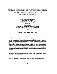
We consider an overlay of peers connected with a general mesh topology. The total number of peers is N . Each peer is connected to NN other peers2 which constitute its neighborhood. A special case is NN = N − 1, which define a fully connected mesh. We consider the presence of one more “special peer” that is the source of the video. The source never receives chunks, so its links are logically unidirectional and it is not part of any neighborhood, i.e., its unidirectional links are additional to the others. Fig. 1 reports two sample topologies. The source distributes a (possibly live) video or TV program. The video is divided in Mc chunks of equal duration emitted periodically. All peers have unit bandwidth (i.e., they can transmit a chunk in exactly the inter-chunk generation time) on the uplink and no limitations on the downlink. We do not consider churn and we focus, as main performance parameter, on the diffusion delay of chunks, which is the delay with which chunks are received by all peers. Formally, if ri is the emission time of chunk Ci , then its diffusion delay is fi = t − ri such that 1 2

The bound comes from the fact that each node can transmit the information only after receiving it, and the number of nodes owning the chunk at most doubles every T . For the sake of simplicity we restrict discussion to n-regular topologies: random graphs with symmetric connectivity and n links per node.

On the Optimal Scheduling of Streaming Applications

(A)

119

(B)

Fig. 1. (A) – General mesh topology with N = 8 and NN = 3; the shaded (pink) area is the neighborhood of the black node; the source is the checkered (yellow) node; (B) – Full mesh with N = 4

all N peers have received Ci . Each peer has a perfect knowledge of the status of its neighbors. The assumptions above means that: i) no global ordering of peers is required; ii) the system is not structured; iii) schedulers’ decisions are independent one another; vi) peers know exactly the subset of chunks already received or being received by all neighbors; and v) signaling delay is negligible. The first scheduling decision is whether a peer pushes information to other peers or if it pulls it from other peers . . . or a mix of the two policies. Sometimes in the literature it is stated that pushing information is a behavior typical of structured systems, and pull methods are more adapt for non-structured overlays. Recent papers like [6,7] instead use push schedulers on non-structured meshes. Indeed, the choice of whether it is better to push or pull information is not related to the structure (or the lack of it) of the system, but to the bandwidth bottleneck, which can create conflicts in scheduling decisions. Push-based systems are suitable for systems where the bottleneck is the uplink, because this guarantees a priori that only one chunk will be scheduled for transmission on the uplink, and that scheduling conflicts arising from the distributed nature of the scheduling will insist on the downlink of other peers. If the situation were reversed (uncommon in networks dominated by ADSL access, but technically possible), then pull-based schedulers would solve a priori the conflict on the downlink, and more bandwidth-endowed uplinks would accommodate scheduling conflicts. Interestingly, a scenario with symmetric upand downlink capacities does not offer an easy logical choice on whether pushing or pulling information is the best choice. We consider push-based schedulers, but we claim that reversing the bottleneck hypothesis, pull-based schedulers which are dual to those we prove optimal in the sequel can be easily derived. 2.2

Formal Notation and Definitions

A system is composed by a set S = {P1 , . . . PN } of N peers Pi , plus a special node called source. Each peer Pi receives chunks Cj from other peers, and send them out to other peers at a rate s(Pi ). The source sends chunks with rate

120

L. Abeni, C. Kiraly, and R. Lo Cigno Table 1. Definitions and symbols used in the paper Symbol S N Mc Pi Ch rh NN fh

Definition The set of all the peers The number of peers in the system The total number of chunks The ith peer The hth chunk The time when the source generates Ch The neighbourhood size The diffusion delay of chunk Ch (the time needed by Ch to reach all the peers) C(Pi , t) The set of chunks owned by peer Pi at time t C  (Pi , t) The set of chunks owned by Pi at time t which are needed by some of Pi ’s neighbours Ni The neighborhood of peer Pi s(Pi ) The upload bandwidth of peer Pi

s(source). The set of chunks already received by Pi at time t is indicated as C(Pi , t). The source, not included in S, generates chunks in order, at a fixed rate λ (Cj is generated by the source at time rj = λ1 j). We normalize the system w.r.t. λ, so that rj = j. Also, we set ∀i, s(Pi ) = s(source) = λ = 1, which is the limit case to sustain streaming. If Dj (t − rj ) is the set of nodes owning chunk Cj at time t, the worst case diffusion delay fj of chunk Cj is defined as the time needed by Cj to be distributed to every peer: fj = min{δ : Dj (δ) = S}. According to this definition, a generic peer Pi will receive chunk Cj at time t with rj + 1 ≤ t ≤ rj + fj . Considering an unstructured overlay t will be randomly distributed inside such interval. Hence, in an unstructured system Pi is guaranteed to receive Cj at most at time rj + fj . To correctly reproduce the whole media stream, a peer must buffer chunks for a time of at least F = max1≤j≤Mc (fj ) before starting to play. For this reason, the worst case diffusion delay F is a fundamental performance metric for P2P streaming systems, and this paper will focus on it. When ∀i, s(Pi ) = λ = 1, at time t the source sends a chunk Cj (with rj = t) to a peer and every peer Pi sends a chunk Ch ∈ C(Pi , t) to a peer Pk . All these chunks will be received at time t + 1. As discussed earlier, the minimum possible diffusion delay fj for chunk Cj is log2 (N )+1. Chunk diffusion is said to be optimal if ∀j, fj = log2 (N )+1 = F . The most important symbols used in this paper are recalled in Table 1.

3

Scheduling Peers and Chunks

In a push-based P2P system, when a peer Pi sends a chunk, it is responsible for selecting the chunk to be sent and the destination peer. The chunk Cj to be sent

On the Optimal Scheduling of Streaming Applications

121

is selected by a chunk scheduler, and the destination peer Pk is selected by a peer scheduler. This paper focuses on algorithms which first select the chunk Cj , and then select a target peer Pk which needs Cj , but the definition of optimality presented in this paper is valid for any chunk-based P2P streaming system. Some well known chunk scheduling algorithms are Latest Blind Chunk, Latest Useful Chunk, and Random Chunk (again, blind or useful). The Latest Blind Chunk algorithm schedules at time t the latest chunk: Cj ∈ C(Pi , t) : ∀Ch ∈ C(Pi , t), rj ≥ rh (Cj is scheduled even if all the other peers already have it). The Latest Useful Chunk (LUc) algorithm selects a chunk that is needed by at least one peer: Cj ∈ C  (Pi , t) : ∀Ch ∈ C  (Pi , t), rj ≥ rh where C  (Pi , t) is a subset of C(Pi , t) containing only chunks that have not already been received (or are not currently being received) by some other peers. The Random Chunk algorithms select a random chunk in C(Pi , t) (Random Blind Chunk) or in C  (Pi , t) (Random Useful Chunk – RUc). Once the chunk Cj to be sent has been selected, the peer scheduling algorithms selects a peer Pk which needs Cj . The most commonly used peer scheduling algorithm is Random Useful Peer, which randomly selects a peer which needs Cj . In theory, the chunk scheduling algorithm can select Pk ∈ S, but in practice peer Pi will only know a subset of all the other peers, and will select Pk from a subset of S called neighborhood. The neighborhood of Pi is indicated as Ni . The case in which ∀i, Ni = S − Pi is special, and corresponds to a fully connected graph. 3.1

Optimal Peer Scheduling

Random peer selection prevents achieving optimality, because the selected peer might be unable to further distribute the chunk. The rationale behind optimal peer selection should be the following: the selected destination peer should be able to immediately take on the role of redistributing the chunk. We define the “Earliest-Latest” peer scheduler (ELp) as follows: ELp selects as target a peer Pl that needs Ch and owns the latest chunk Ck with the earliest generation time rk : Ch ∈ / C(Pl , t) ∧ ∀Pj ∈ Nl , L(Pl , t) ≤ L(Pj , t)

(1)

where L(Pi , t) = maxk {rk : Ck ∈ C(Pi , t)} is the latest chunk owned by or in arrival to Pi at time t. If at time t Pi has not received any chunk yet, L(Pi , t) = 0. If more peers exist that satisfy (1) one is chosen at random. 3.2

Optimal Chunk Scheduling

We show in Theorems 1 and 2 that a LUc/ELp scheduler is optimal in the full mesh case; however, LUc/ELp provides large worst-case diffusion delays when the neighbourhood size is reduced (as will be shown in Section 5). Such a bad behaviour is common to all the LUc schedulers, and is caused by the fact that such schedulers always select the latest useful chunk. Hence, if for some

122

L. Abeni, C. Kiraly, and R. Lo Cigno

reason (such as a restricted neighbourhood size or a limited knowledge of the neighbourhood) a chunk Ck with rk > rh arrives to a peer before Ch is completely diffused, then the peer is not able to diffuse Ch anymore and its diffusion delay is increased by a large amount. In other words, every time that limited knowledge of the neighborhood makes a later chunk arrive to a peer before an earlier one, the diffusion of this latter might be stopped. For this reason, a new scheduling algorithm has been developed to be equivalent to LUc/ELp in the full mesh case, and to perform reasonably well when the graph is not fully connected. The new algorithm is based on a deadline-based chunk scheduling algorithm, named Dl. The Dl scheduling algorithm works based on scheduling deadlines dk associated to every chunk instance. The scheduling deadline is initialized to dk = rk + 2 when the source sends Ck at time rk . The chunk scheduler then works by selecting the chunk Ck with the minimum scheduling deadline: (2) Ck : ∀Ch ∈ C  (Pi , t), dk ≤ dh ; Before sending Ck its scheduling deadline is postponed by 2 time units: dk = dk + 2 (both Pi and the destination peer will see Ck with its new scheduling deadline, while chunk instances present in other peers are obviously not affected). The scheduling strategy based on selecting the chunk with a minimum deadline is known in literature as Earliest Deadline First (EDF), and is mentioned as “Deadline Driven Scheduling” in a seminal paper by Liu and Layland [8], but to the best of our knowledge, it has never been applied with dynamic deadlines in distributed systems. Observation 1. The scheduling deadline dk of a chunk instance Ck at peer Pi is equal to rk + 2d, where d is the number of times that Ck has been selected by the Dl schedulers along the path taken by the chunk till Pi .

4

Analysis with Full Meshes

In this section, some important properties of the LUc/ELp and Dl/ELp scheduling algorithms are proved for the case of a fully connected overlay. In Theorems 1 and 2, it is proved that LUc/ELp achieves optimality, while in Theorem 3 the optimality of Dl/ELp is shown. Lemma 1. When using ELp, ∀i, t ≤ log2 (N + 1) ⇒ ||C(Pi , t)|| ≤ 1. Proof. During an initial transient, at time t the system contains 2t − 1 chunk instances (because at every time instant the source emits a new chunk and all the peers having at least one chunk send a chunk); hence, there are N − (2t − 1) peers having no chunks. By definition, the ELp scheduler selects such peers as targets, hence a peer Pi can have more than 1 chunk only if 2t − 1 > N ⇒ 2t > N + 1 ⇒ t > log2 (N + 1). Lemma 2. If ∀i, s(Pi ) = λ = 1 ∧ Ni = S − Pi , if a LUc/ELp scheduling algorithm is used, then ∀δ, 0 < δ ≤ log2 (N ) ⇒ ||Lj (δ)|| = 2δ−1

On the Optimal Scheduling of Streaming Applications

123

where Lj (δ) = {Pi : maxk {rk : Ck ∈ C(Pi , rj + δ)} = rj } is the set of peers having Cj as their latest chunk at time rj + δ. Proof. The lemma is proved by induction on δ = t − rj , and by considering the latest chunk owned by the peers at time t = rj + δ, so that S is partitioned into three subsets:  – X (δ) = {Lj (i) : i > δ} is the set of peers with latest chunk later than Cj ; – Y(δ) = Lj (δ) is the set of peers having Cj as their latest chunk;  – Z(δ) = {Lj (i) : i < δ} the set of peers with latest chunk earlier than Cj . The above is a partitioning into disjoint subsets, therefore ||X (δ)|| + ||Y(δ)|| + ||Z(δ)|| = ||S|| = N . The lemma can be now proved by induction on δ. Induction base: After chunk Cj is generated by the source at time rj , it is sent out to a peer Pi , which will receive it at time t = rj + 1 ⇒ δ = 1. Hence, Dj (1) = {Pi } ⇒ ||Dj (1)|| = 1 As Cj is the newest chunk in the system, X (δ) is empty and Cj becomes the latest chunk on Pi : ∀Ck ∈ C(Pi , rj + 1), rj > rk Thus, δ = 1 ⇒ ||Lj (δ)|| = ||Dj (δ)|| = 1 = 2δ−1 , ||X (δ)|| = 0 = 2δ−1 − 1. Also note that ||Z(δ)|| = N − 1 > ||X (δ)|| + ||Y(δ)||. Inductive step: First of all, it is easy to notice that ||X (δ − 1)|| ≤ 2δ−2 − 1: in fact, at every time unit a new chunk Ck : rk > rj is generated, and all the peers Pi ∈ X (k − 1) can send their latest chunk to another peer. As a result, ||X (δ − 1)|| will be at most equal to 2||X (δ − 2)|| + 1. But ||X (δ − 2)|| ≤ 2δ−3 − 1 (by induction), so ||X (δ − 1)|| ≤ 2(2δ−3 − 1) + 1 = 2δ−2 − 1 Now, if δ ≤ log2 (N ) , then δ ≤ log2 (N ) ⇒ 2δ ≤ N ⇒ 2(2δ−2 + 2δ−2 ) ≤ N and since ||Lj (δ − 1)|| = 2δ−2 , ||X (δ − 1)|| ≤ 2δ−2 − 1 and ||Z(δ − 1)|| = N − ||X (δ − 1)|| − ||Y(δ − 1)||, the above equation can be rewritten as 2(||X (δ − 1)|| + 1 + ||Y(δ − 1)||) ≤ N ⇒ ||X (δ − 1)|| + ||Y(δ − 1)|| ≤ ||Z(δ − 1)|| − 2 As a result, at δ − 1, ||Z(δ − 1)|| is more than half of N , therefore there are enough peers with latest chunk older than Cj to receive chunks from both X (δ − 1) and Y(δ − 1), so ||Lj (δ)|| = ||Dj (δ)|| = 2δ−1 , hence the claim. Theorem 1. If N = 2i , algorithm LUc/ELp is optimal.

124

L. Abeni, C. Kiraly, and R. Lo Cigno

Proof. By definition, an algorithm is optimal iff ∀j, fj = log2 (N ) + 1. In this case, this means ∀j, fj = i + 1. By Lemma 2, ∀j, δ ≤ log2 (N ) ⇒ ||Lj (δ)|| = 2δ−1 hence, ∀j, ||Lj (i)|| = 2i−1 . As a result, ||Dj (i + 1)|| = 2||Lj (i)|| = 2i = N , and fj = i + 1. Theorem 2. Algorithm LUc/ELp is optimal also if N = 2i . Proof. If N = 2i + n, with n < 2i , by Lemma 2 it comes ∀j, ||Lj (i)|| = 2i−1 . Hence, for δ = i chunk Cj is sent 2i−1 times and chunks with rk > rj are sent 2i−1 − 1 times. As a result, ||Dj (i + 1)|| = 2i , ||X (i + 1)|| = 2i − 1, ||Z(i + 1)|| = 0, and ||Lj (i + 1)|| < ||Dj (i + 1)||. To compute the exact value of ||Lj (i + 1)||, let x be the number of chunks sent by peers in X (i) to peers in Z(i) and let y be the number of chunks sent by peers in Y(i) to peers in Z(i). According to the peer scheduling rules, x + y = ||Z(i)|| (because chunks are sent to peers having the earliest latest chunk). Moreover, ||Lj (i + 1)|| = y + ||Lj (i)|| − (||X (i)|| − x). Hence, ||Lj (i + 1)|| = ||Z(i)|| − x + 2i−1 − (2i−1 − 1 − x) = = (N − 2i−1 − (2i−1 − 1)) − x + 2i−1 − 2i−1 + 1 + x = N − 2i + 1 + 1 = N − 2i + 2 Finally, ||Dj (i + 2)|| = min{N, ||Dj (i + 1)|| + ||Lj (i + 1)|| = 2i + N − 2i + 2} = N Hence, fj = i + 2 = log2 (N ) + 1. Observation 2. If an optimal chunk scheduling is used, all the copies of every chunk Ck are forwarded from time rk to time rk + fk − 2. Based on the optimality of LUc/ELp, it is now possible to prove that Dl/ELp is an optimal algorithm too. This is done by showing that on a full mesh it generates the same schedule as LUc/ELp. Theorem 3. If ∀i, s(Pi ) = λ = 1, ∀i, Ni = S − Pi , then the chunk distribution produced by Dl/ELp is identical to the chunk distribution produced by LUc/ELp. Proof. By contradiction: assume that at any time t0 the chunk distribution produced by Dl/ELp starts to differ from the one produced by LUc/ELp, i.e., assume that Dl at peer Pi at time t0 selects chunk Cj while LUc would select chunk Ck (so, rk > rj ). However, it will be shown that choosing Cj with Dl implies rj ≥ rk contradicting the hypothesis rk > rj . If t0 < log2 (N + 1) , then Lemma 1 guarantees that all chunk schedulers are identical under ELp peer scheduling. If t0 ≥ log2 (N + 1) , we have from the hypotheses that ∀t < t0 the schedules produced by Dl/ELp and LUc/ELp are identical. By definition at time t0 in Pi LUc/ELp choses Ck ∈ C  (Pi , t0 ) : ∀Ch ∈ C  (Pi , t0 )rk ≥ rh .

On the Optimal Scheduling of Streaming Applications

125

Since the source only produces a single chunk at every time unit, rk and rh cannot have the same value, hence rk > rh . To obtain a different schedule Dl/ELp must choose Cj = Ck . Since for t < t0 Dl/ELp produced the same schedule as LUc/ELp, Cj and Ck have been transmitted t0 − rj and t0 − rk times respectively (see Observation 2); hence, di = ri + 2(t0 − ri ) for both Cj and Ck . Since Dl/ELp chooses Cj ∈ C  (Pi , t0 ) : ∀Ch ∈ C  (Pi , t0 )dj ≤ dh we have dj ≤ dk ⇒ rj + 2(t0 − rj ) ≤ rk + 2(t0 − rk ) ⇒ −rj ≤ −rk ⇒ rj ≥ rk which contradicts the hypothesis rk > rj . Observation 3. Note that the Dl scheduler postpones the scheduling deadline by two time units per transmission as dk = dk + 2. If a generic constant q was used instead of 2 and the scheduling deadline was postponed as dk = dk + q, then the last equation in the proof of Theorem 3 would have become rj + q(t0 − rj ) ≤ rk + q(t0 − rk ) ⇒ (q − 1)rj ≥ (q − 1)rk which contradicts rk > rj if q > 1. Hence, if a generic constant q > 1 is used to postpone the scheduling deadline, then Dl/ELp is still equivalent to LUc/ELp. In this sense, Dl can be seen as a whole class of deadline-based algorithms.

5

Neighborhood Restriction and Selected Results

Although both LUc/ELp and Dl/ELp have been proved to provide optimal performance in the case of a fully connected graph their performance in more realistic situations is still unclear. Besides these two algorithms we consider various combinations with LUc, RUc and RUp algorithms for comparison. 5.1

Simulating P2P Streaming and Measuring Performance

The behavior of the scheduling algorithms introduced in Section 3 is analyzed using the SSSim simulator [9], by setting up an overlay of N peers with unit upload and infinite download bandwidth. The source distributes Mc chunks. As explained in Section 2 the performance metric considered in this paper is the worst case diffusion time F , and (as stated in Section 3), a scheduling algorithm is optimal iff F = log2 (N ) + 1. First of all, the algorithms have been simulated on a fully connected graph, as shown in Figure 2. In accordance with Theorems 2 and 3, LUc/ELp and Dl/ELp achieve optimal performance, outperforming the other algorithms (in particular, RUc/ELp achieves a value of fi near the double of the optimal, and all the other algorithms achieved even worse performance). 5.2

Restricting the Overlay

In realistic situations a restricted overlay is used instead of a fully connected graph. Such a restricted overlay is modeled assuming bidirectional relations and

worst case diffusion delay (F)

126

L. Abeni, C. Kiraly, and R. Lo Cigno

Dl/ELp Dl/RUp LUc/ELp LUc/RUp RUc/ELp RUc/RUp 100

10 0

200

400 600 Number of peers (N)

800

1000

Fig. 2. Full mesh overlay; maximum diffusion delay as a function of N; 500 chunks

10000

worst case diffusion delay (F)

worst case diffusion delay (F)

10000

1000

100

Dl/ELp Dl/RUp

LUc/ELp LUc/RUp

RUc/ELp RUc/RUp

1000

100

10

10 10 Neighborhood size (NN)

100

1000 2000 3000 4000 Stream length (Mc) [chunks]

5000

Fig. 3. Worst case chunk diffusion delay of algorithms, with 1000 peers, as a function of: (left) neighborhood size, with 2000 chunks; (right) number of chunks, with NN = 11

a pre-defined number (NN = ||Ni ||) of neighbor nodes. The resulting graph is a random NN -regular graph. In the following simulations, the algorithms are evaluated on 10 instances of the random NN -regular graph. We have verified that confidence intervals were always within 5% of the reported mean values with a confidence level of 90%. The left hand side of Figure 3 shows performance of different streaming algorithms as a function of NN and shows how the LUc/ELp algorithm (which is optimal on a full mesh) is highly sensitive to neighborhood restrictions and performs badly when NN < N − 1. Dl/ELp, on the other hand, works better than all the

On the Optimal Scheduling of Streaming Applications

127

32 30 worst case diffusion delay (F)

chunk loss ratio [%]

10

1

28 26 Dl/ELp Dl/RUp LUc/ELp LUc/RUp RUc/ELp RUc/RUp

24 22 20 18 16

0.1

14 10

15

20 50 Neighborhood size (NN)

100

10

15

20 50 Neighborhood size (NN)

100

Fig. 4. Chunk loss and F as a function of the neighborhood size (N = 10000, D = 32)

other algorithms and is able to achieve values of F near the optimum (which in this case is 11). The right side of Figure 3 shows how the number of chunks affects F for NN = 11 (note that log2 (N ) = 9.9658). Dl/ELp keeps good performance even for long streams, while for several other algorithms fi increases with i (the performance of the algorithm depends on the stream length), hence these distribution mechanism results to be unstable in a streaming context. 5.3

Limiting the Chunk Buffer Size

The only solution to the instability problem is to define a playout delay D, and to discard chunks Cj at time rj + D. This causes some chunk loss (for chunks Cj that would have fi > D), but can make the distribution system stable again. Moreover, the playout delay D can be used to dimension the chunk buffers in the peers (in particular, each peer needs to buffer at most D chunks)3 . Since some chunks can be lost, the performance should be evaluated based on both chunk loss ratio and the maximum delay. Figure 4 plots the chunk loss ratio (left) for the various algorithms as a function of the neighborhood size with D = 32. Note that for NN > 14 the chunk loss ratio for Dl/ELp is 0, showing that it is possible to dimension the chunk buffer size so that it does not affect the algorithm’s performance (to the authors’ best knowledge, this is not possible for the other algorithms). The worst case diffusion time F (right) fastly approaches the optimum with Dl/ELp, while it is obviously 32 for all other algorithms. 3

Implementing the chunks buffer size in the simulator can enable optimizations which allow to simulate larger task sets, hence we move to N = 10000.

128

L. Abeni, C. Kiraly, and R. Lo Cigno

1000

worst case diffusion delay (F)

DL/ELp

DL/RUp

LUc/ELp

LUc/RUp

RUc/ELp

RUc/RUp

100

10 0

0.1

0.2

0.3

0.4 0.5 heterogeneity (h)

0.6

0.7

0.8

0.9

Fig. 5. F as a function of bandwidth heterogeneity (N = 600, Mc = 600)

5.4

Heterogeneous Upload Bandwidth

Finally, we evaluate the performance of Dl/ELp in heterogeneous networks. We use a scenario similar to that of [6]. The system is composed of N =600 nodes, devided in 3 classes based on their upload bandwidth: bandwidth of 2 for (h/3)N nodes4 , bandwidth of 0.5 for (2h/3)N nodes, and unit bandwidth for (1 − h)N nodes, thus keeping the mean bandwidth at 1. We vary h from 0 (homogeneous case) to 1. Figure 5, plotting the diffusion delays for Mc = 600 chunks and an infinite buffer size, shows that Dl/ELp performs better in this specific setting than the other algorithms studied for the whole range of h. These initial studies indicate that Dl/ELp could be a strong contender also in heterogeneous settings. We leave more detailed studies, including studies of the effect of Dl’s increment parameter on performance (see observation 3), for future work.

6

Related Work and Contributions

Optimality of schedulers has been extensively studied in the literature. For the case of full mesh overlay and unit upload bandwidth limits, the generic (i.e., valid for any scheduler) lower bound of (log2 (N ) + 1)T is well known. [1] proves that this bound is strict in a streaming scenario by showing the existence of a centralized scheduler that achieves such bound. A similar proof (although for the case of file dissemination) can be found in [11]. Our work improves on these results by proving 4

In order to validate our results with heterogeneous bandwidth, we implemented our algorithms also in the P2PTVSim [10] simulator. For this reason, we had to use a smaller number of peers and chunks.

On the Optimal Scheduling of Streaming Applications

129

the existence of distributed schedulers (LUc/ELp and Dl/ELp) that achieve the same strict bound. Generic upper bounds as well as upper bounds on the distribution times achieved by different distributed schedulers can also be found in literature. The fundamental work of [12] studies asymptotic properties of distributed gossiping algorithms in a similar setting, showing an upper bound for any pull based algorithm of all the messages in O(Mc + log(N )) time with high probability even for blind algorithms. Generic asymptotic bounds are also shown for blind push based algorithms, although in this case full dissemination cannot be guaranteed. A blind algorithm that distributes chunks with a high probability in (9∗Mc +9∗log2 (N ))T is also shown. Note that this suggest a distribution delay for the individual chunk that grows with Mc . Authors of [11] also evaluate blind distributed strategies in the case of file distribution, showing distribution delays dependent on the number of chunks. [6] studies upper bounds for specific well known algorithms, showing that the combination of random peer selection and LUc achieves asymptotically good delays, however this demonstration is provided in the case of upload bandwidth higher than 1. The distributed LUc/ELp and Dl/ELp schedulers presented in our paper perform significantly better than the generic upper bounds shown in [12] and [11] in that it achieves full diffusion of all chunks in (Mc + log2 (N ))T , i.e. a chunk diffusion delay independent of Mc . It also differs from the streaming algorithms studied in [6], since for LUc/ELp and Dl/ELp this strict delay bound holds for any N (not just asymptotically), and it is valid even in the boundary case of unit upload bandwidth, without relying on redundant source coding. [6] uses ER graphs to model the restricted neighborhood. With N = 600 and NN = 10, authors find that the studied algorithms suffer significant losses. These chunk losses are confirmed by our results (even if our random graph model is slightly different) for the algorithms considered therein. However, we also show (through simulations) that the new Dl/ELp algorithm performs near the optimum with any Mc and any N , even with significant overlay restrictions. Namely, reducing the neighborhood size to any NN >= log2 (N ), our algorithm keeps distributing all chunks with a delay only slightly above the lower bound and always (on all simulated NN -regular random graphs) below 2 ∗ (log2 (N ) + 1)T . Note that the neighborhood of log2 (N ) practically means less than 30 in any reasonable setting.

7

Conclusions and Future Work

This paper presented the formal proof that distributed algorithms can achieve optimal diffusion for streaming applications in unstructured meshes. The paper introduced a class of deadline based algorithms Dl/ELp which are optimal in full meshes and maintain very good properties also in realistic scenarios with small neighborhoods.

130

L. Abeni, C. Kiraly, and R. Lo Cigno

Future work includes on the one hand extending the theoretical results to scenarios with different constraints, including large bandwidth and heterogeneous scenarios, and, on the other hand, exploiting these algorithms to implement real P2P streaming systems.

References 1. Liu, Y.: On the minimum delay peer-to-peer video streaming: how realtime can it be? In: MULTIMEDIA 2007: Proceedings of the 15th international conference on Multimedia, Augsburg, Germany, pp. 127–136. ACM Press, New York (2007) 2. Hefeeda, M., Habib, A., Xu, D., Bhargava, B., Botev, B.: Collectcast: A peer-to-peer service for media streaming. In: ACM Multimedia 2003, vol. 11, pp. 68–81 (2003) 3. Hei, X., Liang, C., Liang, J., Liu, Y., Ross, K.W.: Insights into pplive: A measurement study of a large-scale p2p iptv system. In: Proceedings of the Workshop on Internet Protocol TV (IPTV) services over World Wide Web in conjunction with WWW 2006 (2006) 4. Chu, Y., Ganjam, A., Ng, T.S.E., Rao, S.G., Sripanidkulchai, K., Zhan, J., Zhang, H.: Early experience with an internet broadcast system based on overlay multicast. In: ATEC 2004: Proceedings of the annual conference on USENIX Annual Technical Conference, Boston, MA, June 2004, USENIX Association (2004) 5. Pianese, F., Keller, J., Biersack, E.W.: Pulse, a flexible p2p live streaming system. In: IEEE INFOCOM (2006) 6. Bonald, T., Massouli´e, L., Mathieu, F., Perino, D., Twigg, A.: Epidemic live streaming: optimal performance trade-offs. In: Liu, Z., Misra, V., Shenoy, P.J. (eds.) SIGMETRICS, Annapolis, Maryland, USA, pp. 325–336. ACM, New York (2008) 7. Couto da Silva, A., Leonardi, E., Mellia, M., Meo, M.: A bandwidth-aware scheduling strategy for p2p-tv systems. In: Proceedings of the 8th International Conference on Peer-to-Peer Computing 2008 (P2P 2008), Aachen (September 2008) 8. Liu, C.L., Layland, J.: Scheduling alghorithms for multiprogramming in a hard realtime environment. Journal of the ACM 20(1) (1973) 9. Abeni, L., Kiraly, C., Cigno, R.L.: TR-DISI-08-074: SSSim: Simple and Scalable Simulator for P2P streaming systems. Technical report, University of Trento (2008), http://disi.unitn.it/locigno/preprints/TR-DISI-08-074.pdf 10. The NAPA-WINE Project: P2PTVSim home page, http://www.napa-wine.eu/cgi-bin/twiki/view/Public/P2PTVSim 11. Mundinger, J., Weber, R., Weiss, G.: Optimal scheduling of peer-to-peer file dissemination. J. of Scheduling 11(2), 105–120 (2008) 12. Sanghavi, S., Hajek, B., Massouli´e, L.: Gossiping with multiple messages. In: Proceedings of IEEE INFOCOM 2007, Anchorage, Alaska, USA, May 2007, pp. 2135– 2143 (2007)