On the Relationship of Synaptic Activity to Macroscopic ... - CiteSeerX

Brain Topography, Volume 13, Number 2, 2000

79

On the Relationship of Synaptic Activity to Macroscopic Measurements: Does Co-Registration of EEG with fMRI Make Sense? Paul L. Nunez*^ and Richard B. Silberstein*+^

Summary: A two-scale theoretical description outlines relationships between brain current sources and the resulting extracranial electric field, recorded as EEG. Finding unknown sources of EEG, the so-called "inverse problem", is discussed in general terms, with emphasis on the fundamental non-uniqueness of inverse solutions. Hemodynamic signatures, measured with fMRI, are expressed as voxel integrals to facilitate comparisons with EEG. Two generally distinct cell groups (1 and 2), generating EEG and fMRI signals respectively, are embedded within the much broader class of synaptic action fields. Cell groups 1 and 2 may or may not overlap in specific experiments. Implications of this incomplete overlap for co-registration studies are considered. Each experimental measure of brain function is generally sensitive to a different kind of source activity and to different spatial and temporal scales. Failure to appreciate such distinctions can exacerbate conflicting views of brain function that emphasize either global integration or functional localization. Key words: EEG; ERP; fMRI; PET; Co-registration; Generators; Current sources; Dipole localization.

Introduction Over the past few years, brain science has exhibited an explosive growth in hemodynamic/metabolic data on brain function. In particular, Positron Emission Tomography (PET) and functional Magnetic Resonance Imaging (fMRI) provide excellent spatial resolution, but their temporal resolutions are severely limited by relatively slow responses of brain metabolism. By contrast, electroencephalography (EEG) and magnetoencephalography (MEG) are able to track modulations of current source activity at millisecond time scales, but suffer from poor spatial resolution. An apparently plausible approach for achieving both high spatial and temporal resolution is to combine metabolic and electric/magnetic measures in some way, e.g., by co-registration. Co-registration of EEG with fMRI is currently a popular topic in the brain imaging literature (see reviews by

* The Brain Sciences Institute, Melbourne, Australia. + Dept. of Biophysical Sciences and Electrical Engineering, Swinburne University of Technology, Melbourne, Australia. ^ Brain Physics Group, Dept. of Biomedical Engineering, Tulane University, New Orleans, LA, USA. Accepted for publication: September 21, 2000. Correspondence and reprint requests should be addressed to Prof. Paul L. Nunez, Brain Physics Group, Dept. of Biomedical Engineering, Tulane University, New Orleans, LA 70118, USA. Fax: 01-504-862 8779. Copyright © 2000 Human Sciences Press, Inc.

Rosen et al. 1998 and Liu et al. 1998). One approach is to constrain EEG inverse solutions (e.g., dipole localization) to regions where fMRI indicates relatively large hemodynamic signatures. This approach is partly supported by studies linking metabolic and hemodynamic activity with local neuronal synaptic and electrical events (Rosen et al. 1998). We do not question the existence of this link in many studies. Rather, we emphasize that EEG and MEG are very selective measures of current source activity, often corresponding to small subsets of total synaptic action in tissue volumes and largely independent of action potentials. Increases in neural firing rates may occur with reduced large-scale synchrony of current sources and, as a result, smaller electric or magnetic scalp fields. By contrast, hemodynamic and metabolic measures are believed to increase with neural firing rates. How closely do we expect these disparate measures of brain function to agree? We believe the theoretical and experimental limitations of co-registration require more critical review than we have found in the literature. Does co-registration make sense? The answer may be a sensitive function of the specific scientific questions being addressed. The central purpose of this paper is to outline some of the fundamental physical principles and assumptions involved in co-registration, with the goal of facilitating more realistic experimental design and physiological interpretation of future data. There is general agreement about the physiological sources of EEG and MEG data in broad outline, not in de-

80

tail. Extracranial electric and magnetic fields are known to be generated by brain current source activity, generally producing a current dipole moment in each tissue volume (Nunez 1981, 1995; Nierdermeyer and Lopes da Silva 1999). For purposes of providing a convenient theoretical framework, we may define such elemental tissue volumes as cortical columns of various sizes, fMRI voxels, or volumes at any other spatial scale large enough to contain many current sources, e.g., many synapses. In order to make convenient use of dipole concepts for EEG applications, elemental tissue volume scales should be much smaller than their distances to local scalp. Other factors being equal, tissue volumes close to the scalp surface and producing large dipole moments are much more likely to contribute to extracranial electric or magnetic fields. Each elemental tissue volume produces a dipole moment vector. MEG is much more sensitive to dipole moment vectors tangent to magnetic sensor coils (often roughly tangent to local scalp surface). EEG is more sensitive to dipole moment vectors normal to scalp. Neocortex is often the best candidate structure for unknown sources of large EEG signals for three fundamental reasons (Nunez 1981, 1995; Nierdermeyer and Lopes da Silva 1999): (1) Proximity to recording electrodes or magnetic coils (2) Morphology of cortical pyramidal cells aligned in parallel (3) High density of intracortical and cortico-cortical fibers facilitating synchronous source activity in directions tangent to the cortical surface, often over several tens of cm2. For purposes of this paper, the main point is that current source geometry within volume elements and synchrony of volume elements among themselves over large distances (much larger than a single fMRI voxel diameter) are the main factors determining EEG magnitudes. At least several of these factors may be largely independent of local hemodynamics/metabolism. For example, cortical stellate cells occupy roughly spherical volumes such that associated synaptic sources provide a "closed field" structure. That is, stellate cells are electrically and magnetically invisible to extracranial sensors. Stellate cells constitute only about 15% of the neural population of neocortex (Braitenberg and Schuz 1991; Wilson et al. 1994). However, they apparently make a disproportionate contribution to cortical metabolic activity as a consequence of higher firing frequencies of action potentials (Connors and Gutnick 1990) because metabolism requirements are expected to increase with firing frequency. Thus, one can easily imagine a region of cortical tissue with large metabolic load making no contribution to EEG. Several scenarios suggesting strong EEG signals and weak metabolic signatures also come to mind. EEG can evidently be large if only a few percent of neurons in each cortical column are "synchronously active", provided a large-scale synchrony among different columns produces (effectively) a large dipole sheet in which individual col-

Nunez and Silberstein

umns tend to be phase locked (in selective frequency bands). But, the majority of neurons in each intra-column population may be relatively inactive, producing minimal metabolic signatures. The human alpha rhythm appears to be an example of this phenomenon. The alpha rhythm is strongly attenuated with eye opening over the entire scalp. But it appears implausible that hemodynamic or metabolic activity in primary or secondary visual cortex is actually reduced during visual processing. We suggest that scalp EEG amplitudes and hemodynamic or metabolic activity can change in opposite directions for reasons having to do with the distinct spatial scales and selective frequency bands of cortical "synchrony". Another example is that of neocortical epileptogenic foci during interictal periods. In one study, large focal spikes were observed in the interictal EEG (Olson et al. 1990). In seven of eight children the interictal PET actually showed focal hypometabolism due perhaps to disinhibition of pyramidal cells. In another study of 13 children with lateralized epileptic spikes, regional glucose metabolism measured with PET was not lateralized, suggesting that "metabolic changes associated with interictal spiking cannot be demonstrated with PET with 18F-flurodeoxyglucose…" (Van Bogaert et al. 1998). Apparently, reduction in inhibitory activity near epileptic foci may reduce local metabolic signatures, while at the same time, producing large EEG amplitudes. In the following sections, we address the issue of co-registration in a semi-quantitative manner. The basic physics of EEG and the inverse problems of locating sources are outlined. We formally express fMRI signatures in a similar manner to EEG so as to facilitate comparisons between these disparate measures. We largely ignore the important engineering issue of algorithm efficacy in this paper. For example, the description depends on brain volume integrals rather than matrix equation estimators. New and better algorithms will be developed for future brain imaging, but all algorithms are constrained by fixed physical principles.

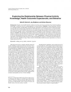
Cell groups generating electric, magnetic, hemodynamic/metabolic signatures Figure 1 outlines relationships between various cell groups and electric (EEG), magnetic (MEG) and hemodynamic/metabolic (MRI, PET) measures of brain function. Causal, correlative and speculative connections are depicted. The different cell groups and their relationships are outlined in this section. Synaptic action fields We make use of the idea of synaptic action fields (Nunez 1974, 1981, 1989, 1995, 2000a,b) to facilitate connec-

Co-registration of EEG with fMRI

81

Figure 1. Double arrows indicate established correlative relationships between behavior/cognition and EEG, MEG, MRI and PET. Excitatory and inhibitory synaptic action fields are defined simply in terms of numbers of active synapses per unit volume (independent of functional significance). By definition, cell groups 1 generate EEG or MEG and cell groups 2 generate MRI or PET. Cell groups 1 and 2, which may or may not be part of networks, are embedded within the larger category (or "culture") of active synapses ("synaptic action fields"). Cell assemblies and cell groups 1 and 2 may or may not overlap. Causal and correlative (may or may not be causal) interactions are indicated by hyphens and slashes, respectively.

tions between brain current sources and scalp potentials. Synaptic action fields are defined as the number densities of active excitatory and inhibitory synapses in tissue volumes, independent of their functional significance. For example, each minicolumn of human neocortex contains about 100 pyramidal cells and a million synapses (Mountcastle 1979). There are perhaps six excitatory synapses for each inhibitory synapse, at least in mouse (Braitenberg and Schuz 1991). If for purposes of discussion, we assume that 10% of all synapses are active at any given time, the excitatory and inhibitory synaptic action densities are about 85,000 and 15,000, respectively, per minicolumn volume. Synaptic action fields, cell groups 1 and 2, and cell assemblies are depicted in figure 1. Cell groups 1 and 2 and cell assemblies are subsets of the synaptic action fields. These subsets may or may not overlap, but all are embedded within synaptic action fields. To use a sociological metaphor, the synaptic action fields form a "culture" composed of various sub-groups at multiple scales of neighborhoods, cities, nations, etc. The introduction of synaptic action fields is motivated by their causal connection to EEG, paths F-1 (fields to cell groups 1) and 1-E (cell groups 1 to EEG/MEG) in

figure 1. EEG frequencies below about 50 Hz are believed to be essentially the modulation frequencies of synaptic action fields around their background levels (Nunez 1995). Higher frequencies in macroscopic tissue volumes appear to be low pass filtered at cellular levels due to capacitive-resistive membrane properties (Nunez 1995)1. Thus, macroscopic synaptic action fields are natural variables to explain scalp potentials. The macroscopic field descriptions are convenient for making contact with macroscopic measures of brain function; at least until new variables with equally robust connections to such data are developed. Theories of behavior and cognition, within the confines of the cell assembly box in figure 1, may be quite distinct from synaptic field concepts. But, putative new variables used to describe such cell assemblies or "networks" must explain data if they are to represent genuine science. If such data include EEG, separate theories will be required to relate new variables either to synaptic fields or to alternate measures closely aligned with scalp data. We do not imply that EEG and synaptic field dynamic behavior are necessarily similar. Quite the contrary, the most complicated synaptic field dynamics (all but the low end of the spatial frequency spectrum) are never recorded

82


ism covers two spatial scales. This approach takes advantage of the columnar structure of neocortex, believed to contain sources making by far the largest contributions to scalp potentials recorded without averaging. However, the description is easily generalized to synaptic action in subcortical tissue. For electrical measurements, the "source strength" of a volume of tissue is given by its electric dipole moment per unit volume (Nunez 1981, 1990, 1995). P( r' , t ) =

Figure 2. The physiological basis for the proposed two-scale description of EEG sources is depicted, indicating relationships between micro-sources at the membrane level, mesoscopic sources at the voxel or column scale, and macro-potentials recorded on the scalp. Volume micro-sources s(r’, w, t) (microamperes/mm3) are generated at membrane surfaces because of synaptic action and passive return current. A cortical voxel (or column of somewhat arbitrary diameter) is located at r’. Micro-sources are located at w within each voxel (or column). As a result of micro-source strengths, synchrony, and geometric distribution within voxels, the voxels produc e di po l e mo m e nt s p e r u nit v olum e P(r’ , t ) (microamperes/mm 2 ), i.e., the strengths of the "mesoscopic sources" produced by voxels. Scalp potential Φ(r, t) is generally given by the weighted integral of P(r’, t) over the entire brain (sum of contributions from each voxel or column). However, voxels closest to electrodes normally make the largest contributions, as described by the weighting function GΦ(r, r’) (or Green’s function) in equation 2.

on the scalp because of spatial filtering by the head volume conductor, physical separation of sensors from sources or unfavorable source geometry, as outlined below. EEG current sources. A two-scale description By our definition, EEG and MEG are generated by (distinct) current sources in cell groups 1. In order to facilitate connections between synaptic current sources at small scales and macroscopic potentials at the scalp, our formal-

1 ws( r' , w, t )dW( w ) W ∫∫∫ W

(1)

Here dW(w) is the tissue volume element inside volume W. s(r’,w, t) is the local volume source current (microamperes/mm3) near membrane surfaces inside tissue volume W with vector location r’. w is the vector location of sources within W. The current dipole moment per unit volume P(r’, t) in a conductive medium is fully analogous to charge polarization in a dielectric (Plonsey 1969; Jackson 1975; Nunez 1981; Malmivuo and Plonsey 1995). Macroscopic tissue volumes satisfy the condition of electroneutrality at EEG frequencies. That is, current consists of movement of positive and negative ions in opposite directions, but the total charge in any large tissue volume is essentially zero (Schwan and Kay 1957; Plonsey 1969)1. Cortical morphology is characterized by its columnar structure with pyramidal cell axons aligned normal to the local cortical surface. Physiology also supports the columnar picture, e.g., correlations between small electrode recordings taken normal to column axes are typically much higher than correlations between recordings at different cortical depths (Abeles 1982; Petsche et al. 1984). Because of this layered structure, it is often convenient to think of the volume elements dW(w) as cortical columns (height ≈ 2-4 mm), as shown in figure 2. For purposes of describing scalp potentials in terms of synaptic sources, the choice of cortical column diameter is somewhat arbitrary. Column diameter should be at least several times smaller than the shortest distance to the scalp surface (≈1 to 2 cm). Small column diameters avoid quadrupole and higher order contributions to scalp potential that would occur with the same column placed in an infinite homogeneous medium. Columns should also be sufficiently small so that pyramidal cell axes within a single column have approximately fixed orientation. On the other hand, column diameter should be large enough to contain a large number of active synapses so treatment of P(r’, t) as a continuous function of cortical location r’ is accurate. For many purposes, anything between the minicolumn (≈ 0.03 mm) and macrocolumn scales (≈ 1 mm) appears acceptable for many applications involving scalp potentials. The minicolumn is defined in terms of lateral spread of axons of inhibitory neurons. The


83

minicolumn has also been proposed as a basic functional unit of neocortex (Mountcastle 1979; Szentagothai 1978). At this relatively small scale, simplifying assumptions about sources s(r’, w, t) within each column are more easily justified, e.g., that s(r’, w, t) is constant in directions perpendicular to column axes. The sources s(r’, w, t) are generally positive and negative due to local inhibitory and excitatory synapses, respectively. In addition to these active sources, the s(r’, w, t) include passive membrane (return) current required for current conservation. Dipole moment per unit volume P(r’, t) has units of current density (microamperes/mm2). For the idealized case of sources of one sign confined to a superficial cortical layer and sources of opposite sign confined to a deep layer, P(r’, t) is roughly the diffuse current density across the minicolumn (Nunez 1981, 1990, 1995). This corresponds roughly to superficial inhibitory synapses and deep excitatory synapses, for example. More generally, minicolumn source strength P(r’, t) is reduced as excitatory and inhibitory synapses overlap along minicolumn axes. But, such complications are fully consistent with generally equating "source strength" to dipole moment per unit volume using equation 1. Neocortical sources may be viewed as a large dipole sheet of perhaps 1500 to 3000 cm2 (covering the entire surface of gyri, fissures and sulci) over which the function P(r’, t) varies continuously with cortical location r’, measured in and out of cortical folds. In some cases, this dipole layer might consist of only a few discrete regions where P(r’, t) is large, e.g., "focal sources". But, more generally, P(r’, t) is distributed over the entire folded surface. Scalp potentials are believed to be generated by the summed activity of P(r’, t), mainly from upper regions of cortex as depicted in figure 2. Magnetic fields are believed due more to intracellular currents (Hamalainen et al. 1993). However, such currents are closely related to s(r’,w, t) by current conservation so a plausible conjecture is that the "magnetic source strength" of each minicolumn is approximately proportional to P(r’, t). Scalp potential may be expressed as a volume integral of dipole moment per unit volume over the entire brain, provided P(r’, t) is defined generally rather than in columnar terms. However, for the important case of dominant neocortical sources, scalp potential may be approximated by the following integral of dipole moment over the neocortical volume Φ( r , t ) = ∫∫∫ G Φ ( r, r') • P( r' , t )dV ( r') V

(2)

If the volume element dV(r’) is defined in terms of cortical columns, the volume integral may be reduced to an integral over the folded cortical surface. The choice of minicolumn scale for the volume element dV(r’) supports

the convenient assumption that P(r’, t) is everywhere normal to the local cortical surface. In purely resistive macroscopic tissue volumes, the time-dependence of potential is simply the weighted sum of all dipole time variations1. The weighting function (vector Green’s function) GΦ(r, r’) contains all geometric and conductive information about the head volume conductor. For the idealized case of sources in an infinite medium of scalar conductivity σ, the Green’s function is G Φ ( r, r') =

r - r' 4 πσ r - r' 3

(3)

The vector GΦ(r, r’) is directed from the center of each minicolumn (located at r’) to scalp location r, as shown in figure 2. The dot product in equation 2 indicates that only the dipole component along this direction contributes to scalp potential. In genuine heads, GΦ(r, r’) is much more complicated. The most common models consist of three or four concentric spherical shells, representing brain, CSF, skull and scalp tissue with different conductivities (Cuffin and Cohen 1979; Nunez 1981; Srinivasan et al. 1996, 1998). In such models, GΦ(r, r’) is expressed in spherical harmonic expansions, or simply as sums over Legendre polynomials for the special case of exclusively radial dipoles, i.e., P(r’, t) oriented normal to model surfaces. More generally, finite element (Yan et al. 1989; Marin et al. 1998) or boundary element methods may be used to estimate GΦ(r, r’). Such numerical methods have employed MRI to determine tissue boundaries (Le and Gevins 1993; Gevins et al. 1994). However, the accuracy of both analytic and numerical methods is limited by incomplete knowledge of tissue conductivities. Some tissues (e.g., white matter and skull) appear to have substantial anisotropic properties so that head conductivity may be a complicated tensor function of location. However, incomplete knowledge of tissue conductivity has largely precluded application of such direction dependent properties to inverse problems. By contrast to EEG, MEG accuracy is mostly limited by noise and the relatively large distances (≅ 2 to 3 cm) between sensor coils and scalp surfaces (Wikswo and Roth 1988). Despite these limitations preventing highly accurate estimates of head Green’s functions GΦ(r, r’), a variety of studies using concentric spheres or numerical methods have provided reasonable quantitative agreement with experiment. These have included estimates of scalp potential due to measured magnitudes of dura or transcortical potentials (Nunez 1981, 1990, 1995), location of known dipoles implanted in epilepsy patients (Cohen et al. 1990), location of dipoles in a physical head model (Leahy et al. 1998) and location of specific somatosensory cortex from scalp potentials using dura imaging algo-

84

rithms (Le and Gevins 1993; Gevins et al. 1994; van Burik 1999). In the later studies, scalp dura estimates were compared with recordings from the dura surface. From these studies and equations 1 and 2, we can reasonably assume that cell groups 1 generally have the following properties: (1) In the case of potentials recorded without averaging, cell groups 1 are mostly close to the scalp surface. Potentials fall off with distance from source regions as demonstrated by equation 3. In genuine heads, tissue inhomogeneity and anisotropy complicate this issue. For example, the low conductivity skull tends to spread currents (and potentials) in directions tangent to its surface. Brain ventricles, the sub-skull CSF layer and skull holes (or local reductions in resistance per unit area) may provide current shunting. But, still we expect sources closest to electrodes generally to make the largest contributions to scalp potentials. (2) Cells are aligned in parallel to encourage large extracranial electric fields due to linear superposition of fields of individual current sources. Thus, column sources P(r’, t) aligned in parallel and synchronously active make the largest contribution to the integral in equation 2 for scalp potential. For example, 1 cm2 crown of a cortical gyrus contains about 110,000 minicolumns, approximately aligned. Over this relatively small region, the angle between P(r’, t) and GΦ(r, r’) in equation 2 exhibits relatively small changes. By "synchronous" sources we mean that the time dependence of P(r’, t) is roughly consistent (e.g., phase locked) over the area in question (e.g., a gyrus crown). In this case, equation 2 implies that individual synchronous column sources add by linear superposition. By contrast, scalp potentials due to asynchronous sources are due only to statistical fluctuations, i.e., imperfect cancellation of positive and negative contributions to the integral in equation 2. The considerations above imply that scalp potential is roughly proportional to the number of synchronous columns (m) plus the square root of number of asynchronous columns (n) (Nunez 1981, 1995). Suppose, for example, that 1% (m ≈ 103) of minicolumns from a single gyrus produce synchronous sources P(r’, t) and the other 99% of minicolumns (n ≈ 105) produce sources with random time variations. A rough estimate is that the 1% synchronous minicolumn sources contribute m/√n or about three times as much to scalp potential measurements as the 99% random minicolumn sources. This is a critical issue for co-registration because metabolic and hemodynamic measures may be equally sensitive to synchronous and asynchronous columns. (3) Concentric spheres models of the human head have been used to estimate the ratio of dura surface to scalp potential (Nunez 1981, 1995; Srinivasan et al. 1996, 1998). Estimates of this ratio for three different brain to skull conductivity ratios (40, 80, 120) are plotted versus area of the dipole source layer in figure 3 (radial dipoles simulat-


ing synchronous gyri source activity). Although the details of these estimates depend on head model assumptions as expected, the generally accepted idea that small regions of synchronous source activity are strongly attenuated between dura and scalp must be predicted by any plausible head model. Dura to scalp potential ratios of roughly two to six have been widely reported for widespread cortical activity like alpha and delta sleep rhythms (Penfield and Jasper 1954; Abraham and Ajmone-Marsan 1958; Cooper et al. 1965; Goldensohn 1979; Nunez 1981). By contrast, the attenuation factor for focal cortical spikes can be 60 or more. We have found only minimal quantitative information on the attenuation factor as a function of active cortical area; the only two experimental points providing both attenuation factor and corresponding cortical surface of which we are aware are the triangles plotted in figure 3. The arrow corresponds to the general clinical observation that a spike area of at least 6 cm2 of cortical gyri (700,000 minicolumns or 70,000,000 neurons forming a dipole layer) must be synchronously active in order to be recorded on the scalp, or at least identified as a "spike" clinically (Cooper et al. 1965; Ebersole 1997). In this case, "synchronously active" is defined experimentally by cortical recordings (ECoG) in the approximate sense that cortical or dura potentials are roughly in phase over the region of interest. This experimental cortical "synchrony" occurs when some fraction of minicolumn sources is approximately in phase. (4) The above estimates and figure 3 are based on the assumption of gyri sources. For dipole layers partly in fissures and sulci, somewhat larger areas are required to produce measurable scalp potentials. First, the four-concentric spheres model predicts that the maximum scalp potential due to a cortical tangential dipole is about 1/3 to 1/5 (depending partly on CSF thickness, which is typically age-related) of the maximum scalp potential due to a radial dipole of the same strength and depth. Second, tangential dipoles tend to be located more in fissures and (deeper) sulci and may also cancel due to opposing directions. Third, and probably most importantly, synchronous dipole layers of "radial" sources covering multiple gyri can easily form, leading to large scalp potentials due to the product P(r’,t)!GΦ(r, r’) having constant sign over the integral in equation 2. (5) The minimum active area of synchronous cortical sources that may be recorded from scalp in ERP studies by averaging over responses to many sensory stimuli depends on several variables. These include dipole moment directions and magnitudes in the source region, source region depth, stimulus to stimulus stationarity of source region and number of stimuli averaged over. The theoretical estimates and experimental data summarized in figure 3 provide estimates of cortical to scalp potential magni-


85

Figure 3. The solid lines are theoretical estimates of the ratio of dura potential to scalp potential, expressed as a function of "synchronous area" of cortical sources. The theoretical curves were generated by assuming cortical dipole layers of constant (mesoscopic) sources in a head model. The model consisted of four concentric spherical shells representing brain, CSF, skull and scalp. Three assumed skull to brain (or scalp) resistivity ratios are shown (40, 80, 120), bracketing the usual estimate of 80 (Nunez 1981). CSF thickness and resistivity ratio were assumed to be 1 mm and 0.2, respectively. The two triangles are experimental points (Abraham and Ajmone-Marsan 1958; Goldensohn 1979). The large arrow indicates the clinical observation that epileptic spikes must be "synchronous" over at least 6 cm2 of cortex in order be recognized on the scalp (Cooper et al. 1965; Ebersole 1997).

tudes as a function of "synchronous" cortical area. In Appendix A, these data are used to estimate the minimum number of evoked potential averages required to extract a cortical signal generated in tissue of a certain size from background EEG. The number of averages required to extract sources occupying less than a few cm2 of cortex may be very large, suggesting that, in common practice, ERP’s involve relatively extensive source regions. (6) The contribution of action potential sources to extracranial potentials and magnetic fields appears to be small due to multi-directional axon geometry and asynchronous timing of firings. The brain stem evoked potential is probably an exception (Nunez 1981). The issue of action potential sources has minimal effect on our formal description, presented here in terms of current sources, mainly independent of origin of these sources.

Cell assemblies As defined here, "cell assembly" or "neural network" indicates a group of neurons or neural masses (e.g., minicolumns, cortico-cortical columns, macrocolumns, etc) for which correlated activity persists over substantial time intervals (say at least several 10’s of milliseconds). Such correlated activity is widely believed to underlie behavior and cognition in some largely unknown way. Cell assemblies involving contiguous neural structures may form more readily. However, assemblies may also involve cortical regions separated by large distances (e.g., 10 to 20 cm), as suggested by steady state (Silberstein et al. 1990; Silberstein 1995a, 1997) and transient evoked or event related potentials (Gevins and Cutillo 1986, 1995; Gevins et al. 1997). The extreme interconnectedness of the brain seems to encourage such

86

widely distributed assemblies. For example, mainly because of the large density of cortico-cortical fibers, the typical "path length" between any two cortical neurons is only two or three synapses (Braitenberg and Schuz 1991). As envisioned here, cell assemblies may overlap so that, for example, a single macrocolumn may be simultaneously part of several assemblies that perhaps operate in different frequency ranges. Cell assemblies may also have hierarchical structure so that, for example, the 100 neurons in a minicolumn (scale, 0.03 mm), the 100 minicolums in a cortico-cortical column (0.3 mm), and (say) 1000 cortico-cortical columns in remote cortical regions (connected by specific cortico-cortical fibers with lengths in the 1 to 20 cm range) may simultaneously form temporary cell assemblies at different spatial scales (Ingber 1995; Nunez 1995, 2000b). The simple definition of synaptic action fields proposed here ignores cell assemblies or neural networks embedded within synaptic fields, achieving a useful separation of partly known and unknown physiology. Synaptic action fields cause current sources in cell groups 1 that generate EEG, irrespective of whether such cell groups are part of cell assemblies associated with behavior/cognition. Large scalp potentials occur because columnar dipole moments are lined up in parallel and synchronously active. There are many details to be discovered. However, the general causal connections F-1 (synaptic field-cell group 1) and 1-E (cell group 1 sources-EEG) of figure 1 rest on relatively solid theoretical and experimental ground (Nunez 1995; Niedermeyer and Lopes da Silva 1999). The synaptic synchrony requirement for large scalp potential production may also favor the recording of synaptic sources that are parts of cell assemblies. However, other source properties, apparently unrelated to functional cell assembly formation, are also important for large scalp potentials and magnetic fields, including dendrite orientation and source depth. The issues of overlapping and hierarchical cell assemblies further complicate the picture. Thus, there may be minimal justification in assuming that EEG primarily records cell assembly (or "neural network") activity by means of the overlap 1/A (cell groups 1 with cell assemblies) and causal connection 1-E (cell groups 1 to EEG/MEG) in figure 1. More likely, EEG originates with a mixture of cell assembly and non-cell assembly synaptic action, i.e., cell groups 1 only partly overlap the cell assemblies responsible for the specific cognition/behavior under study. But, even if no overlap between cell groups 1 and cell assemblies occur, robust correlations between EEG and behavior/cognition (E/B) could occur as a result of contributions of synaptic action fields to both cell groups 1 and cell assemblies, as indicated by paths (F-1, 1-E) and (F-A, A-B) in figure 1. That is, the general "background" synaptic activity might influence both cell groups 1 and cell assemblies to produce correlations (E/B) between


EEG/MEG and behavior/cognition. Similar arguments apply to correlations (M/B) between MRI/PET and behavior/cognition.

EEG dipole localization and co-registration In its currently popular application, co-registration of EEG with fMRI uses "equivalent dipoles" associated with recorded surface potentials or magnetic fields. Our discussion here focuses on the more widely used spontaneous EEG and event related potentials (ERP’s), but arguments concerning MEG and "evoked fields" are similar. ERP’s are obtained by applying series of sensory stimuli: visual, auditory or somatosensory. Scalp potentials are recorded during the interval following each individual stimulus; typical interval times are 0.5 to 1 second. Cognition is viewed as a sequence of processes in which stimulus information is encoded, compared with memory and acted on (Thatcher and John 1977; Gevins and Cutillo 1986, 1995). The components of ERP waveforms are extracted from spontaneous EEG by averaging the potential at each scalp location over the evoked stimuli. As expected, mid-latency components of ERP waveforms appear to be generated mainly in primary sensory cortex. While early deep sources (e.g., in thalamus) are expected (and sometimes recorded with intracranial electrodes), deep sources are not easily recorded at the scalp. Later components of ERP’s, often associated with cognition, may be widely distributed throughout neocortex. The simple ERP averaging procedure appears to originate with the implicit assumption that spontaneous EEG is "noise", uncorrelated to ERP processes. Such assumption may be invalid (Basar 1980; Nunez 1995, 2000b). Nevertheless, many robust connections between ERP’s and cognition have been established over the past 35 years (Gevins and Cutillo 1995). All volume conductor-based algorithms for locating equivalent dipoles of ERP component waveforms must be based on solving equation 2 for dipole moment per unit volume P(r’, t), often represented by one or perhaps several "equivalent dipoles". We have mostly pictured P(r’,t) at the relatively small spatial scale of a minicolumn. However, fMRI voxels are typically several mm in diameter (macrocolumn scale). With EEG or MEG dipole localization, the tissue volume W in equation 1 defining P(r’, t) must be substantially larger than the macrocolumn scale because of accuracy limitations of inverse solutions. Depending on application, we may view P(r’, t) as defined for volumes W roughly in the 1 to 10 cm3 range. The need for large source volumes W may challenge use of the term "dipole"; however many studies with this interpretation have been published so we will tentatively follow this convention. Extra-physical dipole localization methods (not based on any volume conductor model) have also been


87

suggested, e.g., using only statistical criteria like principal components analysis (PCA). Attempts to substitute statistics for physical principles are fundamentally flawed since the transformation from dipole moment to scalp potential is intimately dependent on the head Green’s function, as shown by equation 2. However, PCA may be used effectively as a preprocessing tool, e.g., to estimate the number of uncorrelated field patterns in raw data. Dipole localization requires sampling the scalp potential in equation 2 at discrete times ti and scalp locations re, obtaining estimates Φ(re, ti). Averaged evoked and event related potentials (ERP’s) are given by < Φ( re , tv ) >=

1 N −1 ∑ Φ(re , nT + tv ) N n=0

(4)

Here T is the interval between successive stimuli; tv is latency from stimuli and N is the number of averages. For a typical cognitive experiment, T ≈ 1 sec, and N ≈ 20 averages are obtained for each latency 0 < tv < 0.5 sec, yielding the event related potential waveform at each scalp location re. Since the Green’s function in equation 2 is independent of time, the identical averaging procedure applies to the dipole moment. Thus, inverse solutions based on ERP waveforms yield estimates of , where the subscript v determines ERP component latency. Since the averaging period NT can easily be several minutes, is evidently much more compatible with metabolic or hemodynamic measures than P(r’, t). Typical numbers of averages N and amplitudes Φ of averaged (transient) scalp evoked potentials are the brainstem evoked potential (N ≈ 2000, ≈ 1 µV), visual evoked potential (N ≈ 200, ≈10 µV) and P300 (N ≈20, ≈10 µV). The apparent relationship of these data to active source region areas is discussed in Appendix A. Two general approaches to dipole localization have enjoyed success in specific applications. The so-called "moving dipole" method (Cohen et al. 1990) finds dipoles at a succession of discrete times ti, with no a priori assumption that the different dipole solutions are related. It is based on solving equation 2 for P(r’, ti) for spontaneous EEG (e.g., epileptic spikes) or at discrete latencies tv of ERP waveforms. With the second class of dipole localization method, spatial and temporal properties of scalp potential sample Φ(re, ti) are combined. Various constraints are applied to find the "best" inverse solutions. For example, the time variations of P(r’, ti) or may be constrained so that dipole moments may change strength but not location over some specified time interval, as with the MSA (multiple source analysis, also known as BESA) algorithm (Scherg and von Cramon 1985; Nunez 1990; Ebersole 1997, 1999; Scherg et al. 1999). Other constraints may involve assumed spatial and temporal smoothness of

inverse solutions or forcing solutions to predetermined brain tissue independently implicated by structural (MRI), metabolic or hemodynamic (PET, fMRI) measures. The popular algorithms for obtaining constrained inverse solutions include MUSIC (multiple signal classification) (Mosher et al. 1999) and LORETA (low resolution topographic analysis) (Pascual-Marqui et al. 1994). The Journal of Clinical Neurophysiology (Vol 16, May, 1999) is devoted to EEG source modeling. The fundamental non-uniqueness of the inverse problem in EEG is easily demonstrated by equation 2. Suppose, for example, that a single dipole is assumed to occupy the fixed brain location r’ = r1 over some time interval as a first approximation to measured scalp potential Φ(re, ti). That is, P(r’, t) = P1(t) δ( r’- r1) a1, where P1(t) is the time varying dipole source magnitude and a1 is its fixed direction. With this assumption, equation 2 yields Φ( re , t i ) = P1 (t i )G( re , r1 ) • a 1

(5)

With only one dipole, scalp potential waveforms at all electrode locations re are identical except for amplitude; i.e., simply equal to the time dependence of the single source1. If the single equivalent dipole hypothesis satisfies this test of time dependence over some time interval, it can then be tested spatially. That is, given some volume conductor model of the head, described by either the electric or magnetic Green’s function G(re, r1), find the best fit solution (P1, r1, a1) to the set of E equations obtained from scalp recordings at the E locations re. A dipole solution (P1, r1, a1) consists of six scalar parameters: one for strength P1 , three for location r1, and two for direction a1. Since the number of recording sites (typically 20 to 131) is normally much larger than the number of unknown dipole parameters, the single equivalent dipole hypothesis can be tested for accuracy. If such test is passed, the best-fit solution (P1, r1, a1) may be found. This procedure has been verified for both EEG and MEG with implanted dipoles in epilepsy patients (Cohen et al. 1990) and a physical human skull phantom (Leahy et al. 1999), as well as in numerous computer simulations over the past 25 years or so. Typical dipole location accuracy in patients and phantom is 0.5 to 1.0 cm for MEG and 1.0 to 2.0 cm for EEG when large numbers (≅ 64 or more) of channels are used. By contrast to experiments with known (single) implanted dipole sources, most brain studies involve an unknown distribution of sources. For unknown sources, finding the best-fit "equivalent dipole" from equation 5 is typically quite different from finding a genuine dipole, even when the test for dipole fit is nearly perfect. For example, a spatially extended neocortical source region can often be fit to a single, deeper dipole (Nunez 1981; Ebersole 1997). Despite such limitations, finding dipole direction and general source region can be quite impor-

88


tant clinically (e.g., in screening candidates for epilepsy surgery), provided the "equivalent dipole" is not erroneously interpreted as a genuine dipole (Ebersole 1999). Consider now the case of K assumed discrete dipoles at locations rk with 6K unknown parameters. Equation 2 yields E equations associated with each sample in time. K

Φ( re , t i ) = ∑ Pk (t i )G(re , rk ) • a k k =1

(6)

By contrast to the single dipole, EEG waveforms are no longer associated with individual sources, rather they occur as (unequally) weighted sums of source waveforms Pk(ti). Sophisticated algorithms can solve these equations. But, such solutions are not unique, even when the number of assumed dipoles K is small. A nice demonstration of this non-uniqueness is presented by Mosher et al. (1999). They simulated six thousand combinations of K = 3 source regions Pk(ti) with a three-shell volume conductor model containing a tessellated human cortex used for placing simulated sources. Each source region occupied 1 cm2 of cortical surface on the upper brain surface (in and out of folds) and produced an independent waveform Pk(ti). The number of spatial samples was E = 180. Two results are mainly of interest here. The RAP(regressively applied and projected)-MUSIC algorithm was generally quite successful in locating the centroids of source patches within 2 mm, based on an algorithm rule of minimizing the contiguous area of each source patch consistent with fitting forward solutions. But, sources generally distributed over the entire upper half of neocortex were able to fit the forward solutions (generated by isolated sources) with equal accuracy. Such large differences in estimated source distributions were due only to source modeling assumptions. In a communication to us (1999), Mosher remarked that "users of these algorithms typically prefer focal to distributed solutions." This "preference" for localized sources poses a substantial problem in neuroscience if the critical distinction between "equivalent dipole" and genuine dipole is lost, an idea well appreciated by many professionals in the field (Mosher et al. 1999; Scherg et al. 1999). For example, Ebersole, a neurologist regularly using dipole localization in clinical practice, routinely interprets deep "equivalent dipoles" that are normal to local superficial cortex as large patches of active cortex (Ebersole 1997, 1999; private communication to Nunez 1999). For many EEG phenomena (including most spontaneous rhythms), we suggest that constraining inverse solutions to the neocortical layer is more realistic than the localized dipole constraint. We base this suggestion on intracranial recordings, dura image and spline-Laplacain scalp recordings (providing high spatial resolution) and

estimates of source strengths required for localized sources to produce recordable scalp potentials (Nunez 1981, 1995). To demonstrate this idea, let the neocortical layer be expressed by the radial coordinate of its outer surface R(Ω), where Ω represents two surface coordinates, that is, P(r’, t) ≈ δ[r’-R(Ω)]. In genuine brains, R(Ω) may be a multi-valued function of Ω near some of the deeper (overlapping) cortical folds. To avoid this complication, only outer cortical layer contributions to scalp potential may be assumed as a first approximation. With columnar sources confined to neocortex, the volume integral in equation 2 reduces to the neocortical surface integral Φ( re , t i ) = ∫∫ G Φ [ re , R( Ω ), Ω ] • P[R( Ω ), Ω , t i ]dΩ Ω

(7)

This is a Fredholm integral equation of the first kind (Morse and Feshbach 1953). It can be solved for the unknown dipole moments P[R(Ω), Ω, ti)] as a function of surface location Ω at each sample time ti or as a best fit to a source model with additional constraints like temporal or spatial smoothness. A special case of equation 7 occurs for R(Ω) = constant, approximating the constraint that all sources occur in neocortical gyri. While this constraint is inappropriate for MEG or for some epileptic source activity, it may be satisfactory in a number of EEG applications where gyri sources appear to dominate sources in fissures and sulci. For the important case of (idealized) spherical head models, one may express the unknown dipole moment in a spherical harmonic Yml (Ω) expansion, where Ω represents the spherical coordinates (θ, φ), that is ∞

P( Ω , t i ) = ∑

l

∑ p lm (t i )Ylm ( Ω )

l =1 m =− l

(8)

Here the simplified notation P[R(Ω), Ω, ti)] → P(Ω, ti) is adopted. Substitute equation 8 into equation 7 and label the resulting surface integrals over the Green’s function as glm(re) to obtain ∞

Φ( re , t i ) = ∑

l

∑ p lm (t i ) • g lm (re )

l =1 m =− l

(9)

Exclusion of the l = 0 term in equation 9 is based on the approximation of current conservation in the head (no current flux through the neck). However, such approximation is not required in EEG if a cephalic reference is used. Since the l = 0 term is spatially constant, potential differences measured from paired locations on a sphere do not record any (possible) contribution from the l = 0 term. With suitable truncation of the l sum and smoothing (e.g., spherical splines) appropriate for limited spatial sampling, equation 9 may be solved for the plm(ti) to be


89

used in equation 8 to obtain estimates of dipole moment distribution over the cortical gyri. Such estimates of equivalent cortical sources (similar to dura imaging) may be viewed as the opposite extreme to dipole localization. We are not advocating any particular numerical scheme here or even promoting dura imaging over dipole localization. The purpose of this exercise is to suggest that, in actual EEG practice, one can always fit scalp data to sources exclusively in neocortex or even to sources only in the crowns of gyri surfaces with least square errors approaching zero. In many applications, this surface constraint may be more physiologically realistic than the focal dipole constraint. Cell Groups 2. Co-registration of EEG with fMRI Cell groups 2 are responsible for hemodynamic/metabolic signatures (fMRI and PET) and may be anywhere in the brain. Typically, they show small percentage increases in activity in one brain state relative to a control state; they are "tip of the iceberg" measures of brain function. This hemodynamic/metabolic activity is believed to increase by neurotransmitter action at synapses. If enough cells within voxels act consistently over long enough times, MRI or PET may show voxel "hot spots" with brain state change. Cell groups that are much smaller than voxels and act independently of contiguous cell groups will generally not show up in the image. In order to formally express salient differences between EEG and metabolic/ hemodynamic measures, we may interpret equation 1 as dipole moment per unit volume P(r’, t) at the voxel scale Θ of a hemodynamic/metabolic measure rather than at the minicolumn scale. Furthermore, generalize the synaptic current sources of equation 1 to include action potential sources. Express sources as s = s+- s-, where s+ and s- are positive definite functions depicting sources and sinks, respectively within each voxel dΘ(w). Combine equations 1, 2 and 4 to obtain scalp evoked potential as a volume integral dV(r’) over the entire brain. < Φ( re , tv ) >=

1 N −1 ∑ dV( r')G Φ (re , r') • NΘ n = 0∫∫∫ V

∫∫∫ w[s + (r' , w, nT + tv ) − s − (r' , w, nT + tv )]dΘ( w ) Θ

(10)

The relationship of hemodynamic or metabolic signatures to cellular processes is not well understood. However, for our general purposes, we assume as a first approximation that the fMRI hemodynamic signature can be expressed as an unknown function g[s+(r, w, t), s-(r, w, t), r, w] of the cellular current sources s+(r, w, t), s-(r, w, t) and (explicitly) the voxel location r and location within the voxel w. The first order (linear) approximation to the fMRI

signal M(r, t) at voxel location r may then be expressed as a convolution integral over time (Friston et al. 1998). M( r , t ) = h 0 ( r ) +

T

1 h 1 ( r , τ)dτ Θ ∫0

∫∫∫ g[s + ( r, w , t − τ), s − ( r, w , t − τ), r, w ]dΘ( w ) Θ

(11)

Here h0(r) is a zero order Volterra kernel, essentially the background metabolic signal or "noise" that occurs at voxel location r in the absence of an input signal (e.g., an evoked stimulus). This includes part, but apparently not all, of the Na-K pump that may produce on going non-synaptic sources (Junge 1992). The first order Volterra kernel h1(r,τ) determines the weighting of the input function g[s+(r’, w, t), s-(r’, w, t), r, w] in terms of delay time τ. In other words, if h1(r,τ) were a sharply peaked function at τ = τ0 , the fMRI signature at time t would depend only on input source activity at time τ- τ0. However in practice, h1(r,τ) may be nonzero over perhaps 15 seconds as a result of metabolic inertia, as in the example shown in figure 4a. Thus, the fMRI signature at any time depends on the input history over past times. This accounts for the relatively poor temporal resolution of fMRI. The inner integral in equation 11 is over the volume Θ of the voxel. In the realistic case of a 3-mm scale voxel, voxel scale is similar to that of a macrocolumn. We express the voxel-averaged input as

[

]

u(r , t − τ)=∫∫∫ g s + (r, w , t − τ), s − (r, w , t − τ), r, w dΘ( w ) Θ

(12)

The "hot spots" of an fMRI voxel picture of the brain are obtained using multiple scans and statistical methods to extract the evoked signal ∆M(r) from several confounding influences (noise) including the zero order kernel, low-frequency artifacts and drifts, and whole brain activity (Friston et al. 1998). These statistical methods test the null hypothesis that the first order kernel h1(r, τ) is zero. In the case of nonlinear fMRI studies, the test also applies to the second order kernel h2(r, τ). Since such statistical methods are not directly related to this study, we summarize the fMRI statistical analyses with angle brackets. ∆M ( r ) ≡ < M ( r , t ) − h 0 >

(13)

This response of the fMRI signal to sensory input provided at different rates is estimated from experimental data and analysis published by Friston et al. (1998), summarized in the Appendix of this paper. The comparison of ERP scalp signal, equation 10, with the fMRI voxel picture, equations 11 through 13 is based on the fact that both formalisms are expressed in terms of mea-

90

Figure 4. (a) The first order fMRI kernel, obtained by fitting equation (B.3) (Appendix B) to the experimental kernel measured by Friston et al. (1998). (b) Our estimate of the AC part of the first order fMRI response as a function of frequency, based on the work of Friston et al. (1998).

sured properties at location r. The spatial scales of these measures are similar, several mm for an fMRI voxel diameter and perhaps 5 to 10 mm for a scalp electrode. However, the spatial scale of source activity estimated from scalp potential or external magnetic field is typically much larger than the mm scale because of noise and head model errors, even when such extracranial data is actually generated by one or two localized sources. Comparison of the ERP and fMRI formal expressions suggests the following: (1) Voxels with small current source activity (s+ , s-) make small contributions to both ERP and fMRI pictures; thus "co-registration" of null activity appears valid. (2) Voxels with large activity due to roughly equal sources and sinks with substantial spatial overlap will contribute no measurable scalp potential due to cancellation of s+ and s- in equation 10. But, no such cancellation


is expected in equations 11 or 12 so large metabolic signatures are possible. This might occur in neural structures with morphology unfavorable to producing large dipole moments, e.g.,"closed fields" from structures like hippocampus. The description also applies to non-pyramidal cortical cells (e.g., stellate cells) with high firing rates (Connors and Gutnick 1990) and large metabolic load that apparently make negligible contribution to ERPs. (3) Large, sustained source activity may produce a large hemodynamic/metabolic signatures and large local dipole moments P(r, t) at deep locations, but the electric or magnetic dipoles may not be recorded at the scalp because of attenuation with distance, described by the Green’s function GΦ in equation 3 for the electrical case. (4) Substantial scalp potentials may occur due to voxel activity over times much shorter than the duration of the first order kernel h1(τ) so that no hemodynamic/metabolic signature is obtained. If for example, one is interested in brain activity in the frequency range of normal spontaneous EEG, the fMRI signal will be very severely attenuated compared to the fMRI low frequency response. A crude analysis of the fMRI frequency response is developed in Appendix B and presented in figure 4b. For example, based on the study by Friston et al. (1998), we estimate that the first order response at 10 Hz is lower by about seven orders of magnitude than the first order DC response. (5) Large metabolic signatures may be obtained, but corresponding differences between brain states may be very small, even though neural source activity within voxels is distributed differently. EEG might change by activation of different cell assemblies that make similar contributions to local metabolic load. Or, reduction in inhibitory cell activity may reduce metabolic load, but cause increased dipole moment due to disinhibition of pyramidal cells. For example, this might occur at an epileptogenic focus during interictal periods when large EEG spikes occur, but metabolic activity is lower due to selective loss of inhibitory synaptic action (Olson et al. 1990; Van Bogaert et al. 1998). EEG, MEG, PET, and MRI are selectively sensitive to different kinds of brain activity. In particular experiments and/or brain states, the cell groups 1 and 2 of figure 1 may show substantial overlap. However, there is no requirement that these disparate measures must generally agree. This is illustrated in figure 5, which shows an idealized 25 cm2 cortical surface containing of the order of 500 macrocolumns. (For purposes of this general discussion, it doesn’t matter if some columns are located in fissures and sulci.) Only a few (shaded) columns are assumed to produce substantial hemodynamic power at relatively long time scales (very low frequency components). The remaining columns are assumed to produce source activity mainly in the much higher frequency range of EPs and ERPs. The fMRI signal can be expected


91

Figure 5. An area of cortex is shown containing roughly 500 macrocolumns (small cylinders). The two shaded columns are assumed to produce substantial signal power at low frequencies ("DC"). These generate fMRI signals on roughly 5 to 10 second time scales as indicated by the plot in upper right. On the other hand, scalp potentials are sensitive to all columns with phase synchrony, including columns producing high frequencies. Scalp potentials are given by the weighted sum of all columnar sources, indicated by the ERP-like waveform shown at upper left.

to come only from these shaded columns with large "DC" activity. However, all columns with substantial high frequency phase synchrony contribute to measured scalp potentials as indicated by equation 2. If the cortical area involved is much larger than several cm2, EEG or MEG dipole localization algorithms can be expected to find only fictitious dipoles substantially deeper than the genuine source region. Electric (or magnetic) dipole and fMRI localization can be expected to agree only when

high frequency synchrony and substantial low frequency power occur in the same tissue mass.

Concluding Remarks The arguments presented here suggest two main conclusions: The first applies generally to localization of brain function and, as a result, to many electric or magnetic and hemodynamic or metabolic studies of brain

92

processes. We conjecture that many experimental conditions occur for which putative overlaps of electric/magnetic (cell groups 1 of figure 1), hemodynamic/metabolic measures (cell groups 2) and cell assemblies is small or perhaps absent entirely. The absence of such overlap need not prevent measurement of correlative relationships between experimental measures and behavior/cognition. For example, robust correlations between cognitive processing and event related potentials can occur as a result of common interactions with the background synaptic action fields depicted in figure 1. A similar argument applies to hemodynamic/ metabolic studies. Lack of cell group overlap need not diminish the importance of measured correlations with behavior and cognition. However, comprehensive consideration of the putative overlap can have profound influence on physiological interpretations of these data. We suggest that over-interpretation of activity apparently localized to discrete brain regions may occur if scientists fail to account for the potential implications outlined in figure 1. EEG’s primary strength is excellent temporal resolution, allowing for genuine measures of neocortical dynamic function at millisecond time scales. The spatial resolution of scalp recorded potentials is substantially poorer than that of fMRI; however high resolution EEG, which provide estimates of dura potential can provide spatial resolution in the 2 to 3 cm range (Perrin et 1989; Gevins and Cutillo 1995; Silberstein 1995a,b; Law et al. 1993; Le and Gevins 1993; Gevins et al. 1994; Nunez et al. 1994, 1997, 1999; Babiloni et al. 1996, 1999; Edlinger et al. 1998; van Burik 1999). The measures of 2 to 3 cm scale dynamic cortical activity include frequency spectra, "desynchronization" (selective amplitude reductions), inter-electrode phase relations, correlation dimensions, inter-electrode covariance/coherence, and information/complexity measures. Many of these dynamic measures show a close correspondence to specific cognitive processes or motor tasks. Traditional ERP’s (simple averaging of brain transient responses) make good sense as preliminary entry points to brain dynamics. However, the ERP averaging procedure may eliminate a large part of potential information in the signal (Basar 1980; Ingber 1995; Nunez 2000b). In this sense, using traditional ERP’s for source localization may be viewed as a somewhat unnatural application of EEG, with relatively poor spatial resolution and sacrificing much of EEG’s potential to measure neocortical dynamics with high temporal resolution. The second point specifically concerns co-registration of electric/magnetic with hemodynamic/metabolic activity. Co-registration of time-averaged evoked (or event-related potentials, ERP’s) with fMRI may be partly justified by somewhat similar time course of these measures. Traditional ERP changes associated with cognitive events typically take place during the period roughly 200 to


500 ms following stimuli. Large changes in hemodynamics apparently occur within 2 to 3 seconds of stimuli. It has been suggested that subtle but possibly observable hemodynamic changes may occur within a few hundred milliseconds of the stimulus. If such methods are developed in the future, "event related fMRI" may allow direct comparison and integration of data acquired using traditional behavioral and electrophysiological methods (Rosen et al. 1998; Dale 1999). However, even assuming such technology is developed, several caveats come to mind. Experimental conditions occur for which the required overlap of cell groups 1 and 2 of figure 1 should not be expected, as in the example of figure 5. Furthermore, when genuine co-registration is actually achieved, it should be interpreted conservatively, e.g., as a sub-class of a potentially much larger class of (generally global) activity, as illustrated by the synaptic action field category of figure 1. For example, a successful matching of an ERP equivalent dipole with an fMRI signature suggests that the indicated tissue is probably an important part of the cell assembly underlying the cognitive task. However, such tissue may not be the most important part. It may also be only a small part of a widely distributed network. In fact, most ERP cognitive studies appear to engage large regions of active cortex. We base this suggestion on the spatial distribution of various estimates of dura potentials, including amplitude, phase, covariance and coherence (Gevins and Cutillo 1986, 1995; Silberstein et al. 1990; Silberstein 1995a, 1997; Nunez 1995; Nunez et al. 1997, 1999). Furthermore, scalp potentials generated from small regions of cortex can be very difficult to extract from background EEG without averaging over a prohibitively large number of evoked potentials, as outlined in Appendix A. This implies that the most localized electrical activity is generally not recorded at the scalp. An apparently plausible argument supporting co-registration of fMRI with ERPs is based on the idea that synchronization generally increases with synaptic activity. For example, it has been suggested that high levels of tonic background activity increase synaptic gain, thereby facilitating synchrony. This argument is only superficially persuasive. Does increased "synchrony" necessarily parallel larger EEG amplitudes? This question hinges on precisely what is meant by "synchrony", in particular the spatial scale and frequency band of synchrony. For example, if more "radial" column dipole moments [Pr(r, t) representing components roughly normal to local scalp surface] become phase locked in some frequency band, we generally expect larger scalp potentials in this band. In this sense, equating large-scale "synchrony" with large EEG amplitude is appropriate. On the other hand, higher small-scale "synchrony" of synaptic action or neural firing along column axes can either increase or decrease the dipole moment of columns, depending on the relative locations of


excitatory and inhibitory neurons and synapses as indicated by equation 1 and figure 2. Another issue is that phase locking of column dipole moment vectors pointing in opposite directions can reduce EEG amplitudes. It is well known that EEG "synchrony" is frequency-dependent. Simultaneous reductions in scalp alpha amplitude and coherence together with increases in theta amplitude and coherence over the same scalp regions occur reliably during cognitive task performance (Gevins et al. 1997; Nunez et al. 1997, 1999). Do we expect increases or decreases in fMRI signatures when "synchrony" in different frequency bands moves in opposite directions? Or consider the large reductions in alpha amplitude over the entire scalp (including occipital regions over primary visual cortex) that occur with eye opening. Do we not expect fMRI signatures to increase in primary and secondary visual cortex during visual processing? If so, then increases in fMRI signatures occur at the same time as decreases in large-scale alpha-band synchrony. In summary, we view brain operation as a combination of quasi-local processes allowed by functional segregation and global processes facilitated by functional integration. Co-registration of fMRI with EEG dipole localization can provide useful information about brain function in special brain regions producing large effective "signal to biologic noise ratio" (as defined above) in both ERP and fMRI measures. However, the criteria for such large signal to noise ratios appear to be quite different for ERP and fMRI. Physiological interpretations of co-registration studies may produce very locally biased views of brain function if the severe limitations of co-registration are not fully appreciated. Perhaps new methods combining hemodynamic or metabolic measures with EEG will lead to a more balanced view that takes global function more fully into account. Such methods could combine the localizing ability of fMRI or PET with important EEG/ERP measures like covariance or coherence that can quantify the wide range of locally to globally dominated dynamic behavior occurring in different brain states.

Footnote 1. The two-scale formulation conveniently separates capacitive effects at small scales from possible macroscopic capacitive effects. Within a small volume W of neural tissue, membrane capacitance (or time and space constants) can reduce the separation of micro-sources in equation 1 at frequencies apparently in the 50 to 100 Hz range, thereby reducing columnar dipole moments (Nunez 1981, 1995). However, once dipole moments are fixed, the time-dependence of potential in equation 2 is identical to that of the dipole moment, except for (possibly) a very small phase shift due to capacitive effects in the volume

93

conductor (imperfect electroneutrality). The phase shift due to capacitive effects in a macroscopic medium of conductivity σ and dielectric constant κ is estimated as follows. Let ω ≅ 2πx10 Hz be the angular field frequency, ε0 = 8.85x10-12 F/m the permittivity of free space, the relative dielectric constant of cortical tissue at low frequencies κ ≅ 106 to 107, and cortical conductivity σ ≅ 1/3 ohm-1 m-1. Based on these parameters taken from the literature (Schwan and Kay 1957), the ratio of displacement (capacitive) current to conduction current (Jackson 1975) is estimated to be ωκε0/σ ≅ 0.017 to 0.0017. The phase difference between a macroscopic current source (or dipole moment per unit volume) and potential is the inverse tangent of this ratio, or approximately 0.1 to 1.0 degree based on measured properties of macroscopic tissue.

Appendix A. Relationship between Size of Source Region and Number of Averages Necessary to Extract Evoked Potentials from Background EEG Here we present a crude model based on cortical sources of spontaneous EEG and EPs or ERPs in a four concentric sphere model of the head. We assume that (1) cortical sources form synchronous (radial) dipole layers of surface area A (2) evoked potentials consist of stationary signals superimposed on spontaneous EEG, treated as uncorrelated noise. While these assumptions are not fully accurate, they allow for the following (very approximate) magnitude estimates. Variables SD Maximum dura potential magnitude of spontaneous EEG. For the rough estimates presented here, SD may be either transcortical potential or potential with respect to a distant reference. SS Maximum scalp potential magnitude of spontaneous EEG. ED Maximum dura potential of a single trial evoked potential. ES Maximum scalp potential of a single trial evoked potential. RS Ratio of dura to scalp potential for spontaneous EEG. This ratio is a function of the synchronous source area AS. The ratio may be estimated from figure 3 and/or clinical EEG observations (RS ≡ SD/ SS). RE Ratio of dura to scalp potential for single trial evoked potential. RE is a function of the synchronous source area AE ( RE ≡ ED/ES ). N Number of trials averaged to obtain EP or ERP. B Attenuation factor of scalp spontaneous EEG (due to averaging) required for observation of averaged EPs in background EEG (B ≈√N ES/SS).

94


Estimates From the definitions above, the number of averages needed to attenuate the effects of background EEG (or amplify the EP signal) with factor B is  R S  N ≈ B E D   R S ED 

2

(A1)

Suppose a single trial visual evoked potential occupies 1 cm2 of cortex and produces columnar dipole moments ten time larger than background (spontaneous) EEG that is produced in a dipole layer of area > 20 cm2, ED ≈ 10 SD. Assume that we require an attenuation factor B = 10 to properly observe the visual evoked potential. From figure 3, we estimate RE ≈ 50 (taking a high end estimate since visual cortical columns have substantial tangential dipole moments) and RS ≈ 5. Equation A1 yields N ≈ 100 averages for a 1 cm2 source region. To record an evoked potential from a 1 mm2 source region with similar assumptions, RE ≈ 500 and a similar estimate yields N ≈ 10,000 averages for a 1 mm2 source region.

Appendix B. Estimate of the fMRI frequency response The following summary and calculations are based on the theoretical-experimental work of Friston et al. (1997). To simplify the notation, the spatial dependence of variables is implicit. A second order approximation to the fMRI (output) signal y(t) at some voxel due to neuronal (input) activity may be expressed T

T

0

0

y(t ) ≈ h 0 + ∫ h 1 ( τ)u(t − τ)dτ + ∫ u(t − τ1 )dτ1 T

2 ∫ h (τ1 , τ 2 )u(t − τ 2 )dτ 2 0

h 1 ( τ) ≈ At 3 e − at − Bt 3 e − bt

(B3)

The following parameters provide a reasonable fit to the data obtained for a 3-mm voxel in the left superior temporal gyrus: A = 2.05007 sec-3, B = 0.00428105 sec-3, a = 1.07143 sec-1, b = 0.30000 sec-1. The estimated first order kernel is shown in figure 4a. The simple form equation B3 allows easy evaluation of the integrals in equation 1 in symbolic terms when T >> a-1 and b-1, and the input function is of the form u(t ) = 1 + cos(ωt )

(B4)

Combining equations B3, B4 and B1 yields the zero order plus first order response function y(t) in terms of the input frequency B  A y(t ) ≈ h 0 + 6 4 − 4  + Amp(ω )Cos[ωt − θ(ω )] a b  (B5) The response consists of the (stimulus off) zero order signal h0 plus DC response plus AC response. The AC response is given by Amp(ω ) ≈ 2

 24Aaω(a 2 − ω 2) 24Bbω(b 2 − ω 2)   + − 4  (a 2 + ω 2)4  b 2 + ω 2) (   2  6A(a 2 − 6a 2ω 2 + ω 2) 6B(b 2 − 6b 2ω 2 + ω 2 )   − 4 4   a 2 + ω 2) b 2 + ω 2) ( (  

(B6)

In the DC limit,

(B1)

Here T is the tissue "memory" and h0, h1 and h2 are the zero, first and second order Volterra kernels, respectively. These were estimated in an fMRI experiment with a subject listening to words repeated at five different rates. The zero order kernel is the hemodynamic signal that occurs with no known input function, essentially brain "noise" from the viewpoint of this experiment. Somewhat surprisingly, the experimental second order kernel was found to be proportional to the square of the first order kernel h 2 ( τ1 , τ 2 ) ∝ h 1 ( τ1 )h 1 ( τ 2 )

We approximate the experimental first order kernel presented graphically in Friston et al. (1997) by the function

(B2)

B  A Amp( 0) ≈ 6 4 − 4  a b 

(B7)

For high frequencies (ω> > a, b) Amp(ω ) →

6 / A − B/ ω4

(B8)

Using numerical values from the Friston et al. (1997) experiment in equation B5 yields y(t ) ≈ 152 + Amp(ω )Cos[ωt − θ(ω )]

(B9)

The function Amp(ω) is plotted versus frequency f =


ω/2π in figure 4b. In summary, the ratio of the amplitudes of responses to noise amplitude is roughly 6 ≈ 4 × 10 −2 152 0.007 1 − Hz response ≈ ≈ 5 × 10 −5 152 8 × 10 −7 10 − Hz response ≈ ≈ 5 × 10 −9 152 DC response ≈

References Abeles, M. Local Cortical Circuits. New York: Springer-Verlag, 1982. Abraham, K. and Ajmone-Marsan, C. Patterns of cortical discharges and their relation to routine scalp electroencephalography. Electroenceph. clin. Neurophysiol., 1958, 10: 447-461. Babiloni, F., Babiloni, C., Carducci, F., Fattorini, L., Onorati, P. and Urbano, A. Spline Laplacian estimate of EEG potentials over a realistic magnetic resonance-constructed scalp surface model. Electroenceph. clin. Neurophysiol., 1996, 98: 204-215. Babiloni, C., Carducci, F., Cincotti, F., Rossini, P.M., Neuper, C., Pfurtscheller, G. and Babiloni, F. Human movement-related potentials vs desynchronization of EEG alpha rhythm: a high-resolution study. NeuroImage, 1999, 16: 658-665. Basar, E. EEG Brain Dynamics. Relation Between EEG and Brain Evoked Potentials. Amsterdam: Elsevier, 1980. Braitenberg, V. and Schuz, A. Anatomy of the Cortex. Statistics and Geometry. New York: Springer-Verlag, 1991. Cohen, D., Cuffin, B.N., Yunokuchi, K., Maniewski, R., Purcell, C., Cosgrove, G.R., Ives, J., Kennedy, J.G. and Schomer, D.L. MEG versus EEG localization test using implanted sources in the human brain. Ann. Neurol., 1990, 28: 811-817. Connors, B.W. and Gutnick, M.J. Intrinsic firing patterns of diverse neocortical neurons. Trends in Neuroscience, 1990, 13: 99-104. Cooper, R., Winter, A.L., Crow, H.J. and Walter, W.G. Comparison of subcortical, cortical, and scalp activity using chronically indwelling electrodes in man. Electroenceph. clin. Neurophysiol., 1965, 18: 217-228. Cuffin, B.N. and Cohen, D. Comparison of the magnetoencephalogram and electroencephalogram. Electroenceph. clin. Neurophysiol., 1979, 47: 136-146. Dale, A.M. Optimal experimental design for event-related fMRI. Human Brain Mapping, 1999, 8: 109-114. Ebersole, J.S. Defining epileptogenic foci: past, present, future. Journal of Clinical Neurophysiology, 1997, 14: 470-483. Ebersole, J.S. The last word. Journal of Clinical Neurophysiology, 1999, 16: 297-302. Edlinger, G., Wach, P. and Pfurtscheller, G. On the realization of an analytic high resolution EEG. IEEE Trans. Biomed. Eng.,1998, 45: 736-745. Friston, K.J., Josephs, O., Rees, G. and Turner, R. Nonlinear event-related responses in fMRI. Magnetic Resonance in Medicine, 1998, 39: 41-52..

95

Gevins, A.S. and Cutillo, B.A. Signals of cognition. In: F.H. Lopes da Silva (Ed.), Handbook of Electroencephalography and Clinical Neurophysiology, Amsterdam: Elsevier, 1986, Vol. 2: 335-381. Gevins, A.S. and Cutillo, B.S. Neuroelectric measures of mind. In: P.L. Nunez (author), Neocortical Dynamics and Human EEG Rhythms, New York: Oxford University Press, 1995: 304-338. Gevins, A.S., Le, J., Martin, N., Brickett, P., Desmond, J. and Reutter, B. High resolution EEG: 124 channel recording, spatial enhancement, and MRI integration methods. Electroenceph. clin. Neurophysiol., 1994, 90: 337-358. Gevins, A.S., Smith, M.E., McEvoy, L. and Yu, D. High-resolution mapping of cortical activation related to working memory: effects of task difficulty, type of processing, and practice. Cerebral Cortex, 1997, 7: 374-385. Goldensohn, E.S. Neurophysiological substrates of EEG activity. In: D.W. Klass and D.D. Daly (Eds.), Current Practice of Clinical Electroencephalography. New York: Raven Press, 1979: 421-439. Hamalainen, M., Hari, R., Ilmoniemi, R.J., Knuutila, J. and Lounasmaa, O.V. Magnetoencephalography-theory, instumentation, and applications to noninvasive studies of the working human brain. Reviews Modern Physics, 1993, 65: 413-497. Ingber, L. Statistical mechanics of multiple scales of neocortical interactions. In: P.L. Nunez (Author), Neocortical Dynamics and Human EEG Rhythms, New York: Oxford University Press, 1995: 628-681. Jackson, J.D. Classical Electrodynamics 2nd Ed, New York: Wiley, 1976. Junge, D. Nerve and Muscle Excitation, Sunderland, Mass: Sinauer Associates, 1992, 3rd Ed: 263. Law, S.K., Nunez, P.L. and Wijesinghe, R.S. High resolution EEG using spline generated surface Laplacians on spherical and ellipsoidal surfaces. IEEE Trans. Biomed. Eng., 1993, 40: 145-153. Le, J. and Gevins, A.S. Method to reduce blur distortion from EEGs using a realistic head model. IEEE Trans. Biomed. Eng., 1993, 40: 517-528. Leahy, R.M., Mosher, J.C., Spencer, M.E., Huang, M.X. and Lewine, J.D. A study of dipole localization accuracy for MEG and EEG using a human skull phantom. Electroenceph. clin. Neurophysiol., 1999, 107: 159-173. Liu, A.K., Belliveau, J.W. and Dale, A.M. Spatiotemporal imaging of human brain activity using functional MRI constrained magnetoencephalography data: Monte Carlo simulation. Proceedings National Academy of Sciences USA, 1998, 95: 8945-8950. Malmuvino, J. and Plonsey, R. Bioelectromagetism. New York: Oxford University Press, 1995. Morse, P.M. and Feshbach, H. Methods of Theoretical Physics, Part I. New York: McGraw-Hill, 1953. Mountcastle, V.B. An organizing principle for cerebral function: the unit module and the distributed system. In: F.O. Schmitt and F.G. Worden (Eds.), The Neurosciences 4th Study Program, Cambridge, MA: MIT Press, 1979. Marin, G., Guerin, C., Baillet, S., Garnero, L. and Meunier, G. Influence of skull anisotropy for the forward and inverse problem in EEG: Simulation studies using FEM on realistic

96

head models. Human Brain Mapping, 1998, 6: 250-269. Mosher, J.C., Baillet, S. and Leahy, R.M. EEG source localization and imaging using multiple signal classification approaches. Journal of Clinical Neurophysiology, 1998, 16: 225-238. Niedermeyer, E. and Lopes da Silva, F.A. Electroencephalography: Basic Principles, Clinical Applications and Related Fields. 4th Ed. Baltimore, Maryland: Urban and Schwarzengerg, 1999. Nunez, P.L. The brain wave equation: A model for the EEG. Mathematical Biosciences, 1974, 21: 279-297. Nunez, P.L. Electric Fields of the Brain: The Neurophysics of EEG. New York: Oxford University Press, 1981. Nunez, P.L. Generation of human EEG by a combination of long and short range neocortical interactions. Brain Topography, 1989, 1: 199-215. Nunez, P.L. Localization of brain activity with EEG. In: S. Sato (Ed.), Advances in Neurology, Magnetoencephalography, Raven Press, New York, 1990, Vol. 54: 39-65. Nunez, P.L. Neocortical Dynamics and Human EEG Rhythms. New York: Oxford University Press, 1995. Nunez, P.L. Toward a quantitative description of large scale neocortical dynamic function and EEG. Behavioral and Brain Sciences, target article, 2000, 23: 371-398. Nunez, P.L. Neocortical dynamic theory should be as simple as possible, but not simpler. Behavioral and Brain Sciences, response to commentary on target article by 18 neuroscientists, 2000, 23: 415-437. Nunez, P.L., Silberstein, R.B., Cadusch, P.J., Wijesinghe, R.A., Westdorp, A.F. and Srinivasan, R. A theoretical and experimental study of high resolution EEG based on surface Laplacians and cortical imaging. Electroenceph. clin. Neurophysiol., 1994, 90: 40-57. Nunez, P.L., Srinivasan, R., Westdorp, A.F., Wijesinghe, R.S., Tucker, D.M., Silberstein, R.B. and Cadusch, P.J. EEG coherency I: Statistics, reference electrode, volume conduction, Laplacians, cortical imaging, and interpretation at multiple scales. Electroenceph. clin. Neurophysiol., 1997, 103: 499-515. Nunez, P.L., Silberstein, R.B., Shi, Z., Carpenter, M.R., Srinivasan, R., Tucker, D.M., Doran, S.M., Cadusch, P.J. and Wijesinghe, R.S. EEG coherency II: Experimental comparisons of multiple measures. Clinical Neurophysiol., 1999, 110: 469-486. Olson, D.M., Chugani, H.T., Shewmon, D.A., Plelps, M.E. and Peacock, W.J. Electrocorticographic confirmation of focal positron emission tomography abnormalities in children with epilepsy. Epilepsia, 1990, 31: 731-739. Pascual-Marqui, R.D., Michel, C.M. and Lehmann, D. Low resolution electromagnetic topography: a new method for localizing electrical activity in the brain. International Journal Psychophysiology, 1995, 18: 49-65. Penfield, W. and Jasper, H.D. Epilepsy and the Functional Anatomy of the Human Brain. London: Little, Brown and Co, 1954. Perrin, F., Pernier, J., Bertrand, O. and Echallier, J.F. Spherical splines for scalp potential and current density mapping. Electroenceph. clin. Neurophysiol., 1989, 72: 184-187. Petsche, H., Pockberger, H. and Rappelsberger, P. On the search for sources of the electroencephalogram. Neuroscience, 1984, 11: 1-27.


Plonsey, R. Bioelectric Phenomena. New York: McGraw-Hill, 1969. Rosen, B.R., Buckner, R.L. and Dale, A.M. Event-related functional MRI: Past, present and future. Proceedings National Academy of Sciences USA, 1998, 95: 773-780. Thatcher, R. and John, E. Functional Neuroscience. Vol. 1. Foundations of Cognitive Processes. Hillsdale, New Jersey: Erlbaum, 1977. Scherg, M. and von Cramon, D. Two bilateral sources of late AEP as identified by a spatiotemporal diploe model. Electroenceph. clin. Neurophysiol., 1985, 62: 32-44. Scherg, M., Bast, T. and Berg, P. Multiple source analysis of interictal spikes: goals requirements, and clinical value. Journal of Clinical Neurophysiology, 1999, 16: 214-224. Schwan, H.P. and Kay, C.F. Capacitive properties of body tissues. Circulation Research, 1957, 5: 439-443. Silberstein, R.B. Steady-state visually evoked potentials, brain resonances, and cognitive processes. In: P.L. Nunez (Author), Neocortical Dynamics and Human EEG Rhythms. Oxford University Press, 1995a: 272-303. Silberstein, R.B. Neuromodulation of neocortical dynamics. In: P.L. Nunez (Author), Neocortical Dynamics and Human EEG Rhythms. Oxford University Press, 1995b: 591-627. Silberstein, R.B. The steady state visually evoked potential, neocortical dynamics and cognitive function. Brain Topography Today. In: Y. Koga, K. Nagata and H. Hirata (Eds.), Amsterdam: Elsevier Science, 1997: 34-38. Silberstein, R.B., Schier, M.A., Pipingas, A., Ciorciari, J., Wood, S.R. and Simpson, D.G. Steady-state visually evoked potentials associated with a visual vigilance task. Brain Topography, 1990, 3: 337-347. Srinivasan, R., Nunez, P.L., Tucker, D.M., Silberstein, R.B. and Cadusch, P.J. Spatial sampling and filtering of EEG with spline-Laplacians to estimate cortical potentials, Brain Topography, 1996, 8: 355-366. Srinivasan, R., Nunez, P.L. and Silberstein, R.B. Spatial filtering and neocortical dynamics: estimates of EEG coherence. IEEE Trans. Biomed. Eng., 1998, 45: 814-826. Szentagothai, J. The neural network of the cerebral cortex: A functional interpretation. Proceedings of the Royal Society of London, 1978, B201: 219-248. Van Bogaert, P., Wikler, D., Damhaut, P., Szliwowski, H.B. and Goldman, S. Cerebral glucose metabolism and centrotemporal spikes. Eplilepsy Research, 1998, 29: 123-127. Van Burik, M.J. Physical Aspects of EEG, Proefschrift Universiteit Twente, Enschede, the Netherlands, 1999. Wikswo, J.P. and Roth, B.J. Magnetic determination of the spatial extent of a single cortical current source: A theoretical analysis. Electroencephalography and Clinical Neurophysiology, 1988, 69: 266-276. Wilson, F.A., O’Scalaidhe, S.P. and Goldman-Rakic, P.S. Functional synergism between putative gamma-aminobutyrate containing neurons and pyramidal neurons in prefrontal cortex, Proceedings National Academy of Sciences USA, 1994, 26: 4009-4013. Yan, Y., Nunez, P.L. and Hart, R.T. Finite element model of the human head: scalp potentials due to dipole sources. Medical and Biological Engineering and Computing, 1991, 29: 475-481.

On the Relationship of Synaptic Activity to Macroscopic ... - CiteSeerX

On the Relationship of Synaptic Activity to Macroscopic ... - CiteSeerX

Suggest Documents

Relating Macroscopic Measures of Brain Activity to Fast ... - CiteSeerX

Enrichment of Conserved Synaptic Activity-Responsive ... - CiteSeerX

Enrichment of Conserved Synaptic Activity-Responsive ... - CiteSeerX

On the Approach to Thermal Equilibrium of Macroscopic ... - CiteSeerX

Impact of Background Synaptic Activity on

Linking Network Activity to Synaptic Plasticity

SYNAPTIC ACTIVITY OF FROG RETINAL

Exploring the Relationship Between Physical Activity ... - CiteSeerX

Phosphodiesterase Inhibition to Target the Synaptic ... - CiteSeerX

Relationship between developmental synaptic ...

Structureâactivity relationship analysis of antioxidant ... - CiteSeerX

Structure-Activity Relationship of Staurosporine Analogs ... - CiteSeerX

From Individual Stochastic Processes to Macroscopic ... - CiteSeerX

Modulation of spinal cord synaptic activity by tumor ... - CiteSeerX

Dependent Synaptic Activity - Semantic Scholar

Synaptic activity-responsive element in the Arc

Macroscopic Taphonomic Alterations to Human Bone ... - CiteSeerX

The macroscopic yield behaviour of polymers - CiteSeerX

Relationship between Texture and Macroscopic Transformation Strain ...

A realistic experiment to demonstrate macroscopic ... - CiteSeerX

Spontaneous Glutamatergic Synaptic Activity ...

Synaptic Background Activity Enhances the ... - Alain Destexhe

Quantification of proliferative activity in relationship to

The role of microglia in synaptic stripping and synaptic ... - CiteSeerX

On the Relationship of Synaptic Activity to Macroscopic ... - CiteSeerX