On the spectrum of a class of quantum models

epl draft

On the spectrum of a class of quantum models Alexander Moroz

arXiv:1209.3265v3 [quant-ph] 18 Dec 2012

Wave-scattering.com

PACS PACS PACS

03.65.Ge – Solutions of wave equations: bound states 02.30.Ik – Integrable systems 42.50.Pq – Cavity quantum electrodynamics; micromasers

Abstract – The spectrum of any quantum model which eigenvalue equation reduces to a threeterm recurrence, such as a displaced harmonic oscillator, the Jaynes-Cummings model, the Rabi model, and a generalized Rabi model, can be determined as zeros of a corresponding transcendental function F (x). The latter can be analytically determined as an infinite series defined solely in terms of the recurrence coefficients.

Introduction. – The present work deals with a class where Aj are in general matrix coefficients. Indeed, on ˆ char- comparing the same powers of z on both sides of (1), the R of quantum models described by a Hamiltonian H consecutive a ˆ† a ˆ, a ˆ† , and a ˆ terms in (6) lead to ncn , cn−1 , acterized in that the eigenvalue equation and (n + 1)c terms in the recurrence (2), respectively. n+1 ˆ = Eφ Hφ (1) Then the eigenvalue equation (1) reduces to a coupled sysin the Bargmann Hilbert space of analytical functions B tem of ordinary differential equations [1, 4, 5]. The model Hamiltonian (6) encompasses many prominent examples, [1, 2] reduces to a three-term difference equation such as a displaced harmonic oscillator [1], the Rabi model cn+1 + an cn + bn cn−1 = 0 (n ≥ 0). (2) [1, 6], the Jaynes and Cummings (JC) model proposed as ∞ Here {cn }n=0 are the sought expansion coefficients of a an approximation to the Rabi model [7], and a generalized Rabi model [8]. The Rabi model describes the simplest inphysical state described by an entire function teraction between a cavity mode with a bare frequency ω ∞ X n φ(z) = cn z . (3) and a two-level system with a bare resonance frequency ω0 . The model is characterized by the Hamiltonian [1, 6, 8], n=0 ˆ R = ~ωˆ The recurrence coefficients an and bn are functions of H a† a ˆ + λσ1 (ˆ a† + a ˆ) + µσ3 , (7) model parameters and we require that bn 6= 0. In what follows, models of the class R are characterized by the re- where λ is a coupling constant, and µ = ~ω0 /2. In what currence coefficients having an asymptotic power-like de- follows we assume the standard representation of the Pauli matrices σj and set the Planck constant ~ = 1. pendence Our main results is that the spectrum of any quantum an ∼ anδ , bn ∼ bnυ (n → ∞), (4) model from R can be obtained as zeros of a transcendental wherein 2δ > υ and τ = δ − υ ≥ 1/2, which guarantees function defined by infinite series limn→∞ bn /an = 0. ∞ X The conventional boson annihilation and creation operF (x) ≡ a0 + ρ1 ρ2 . . . ρk (8) ators a ˆ and a ˆ† satisfying commutation relation [ˆ a, a ˆ† ] = 1 k=1 are represented in the Bargmann Hilbert space B as [1, 2] solely in terms of the coefficients of the three-term recur∂ † , a ˆ → z. (5) rence in eq. (2) [9]: a ˆ→ ∂z b1 Therefore, the class R comprises among others singleρ1 = − , ρl = ul − 1, u1 = 1, a1 mode boson models represented by 1 ul = , l ≥ 2. (9) ˆ = A1 a H ˆ† a ˆ + A2 a ˆ† + A3 a ˆ + A4 , (6) 1 − ul−1 bl /(al al−1 ) p-1

Alexander Moroz B [1, 5]. Our approach differs from earlier studies [1, 5, 8] in that our focus is initially on the truly three-term part of the recurrence (2) for n ≥ 1. This would enable us to remain in B for any value of physical parameters. The remaining n = 0 part of the recurrence (2), which reduces to a relation between c1 and c0 , then becomes the boundary condition for φ ∈ B defined by the n ≥ 1 solutions of the recurrence (2). In virtue of the Perron and Kreuser generalizations (Theorems 2.2 and 2.3(a) in ref. [3]) of the Poincar´e theorem (Theorem 2.1 in ref. [3]), the difference equation (2) (considered for n ≥ 1) possesses in our case two linearly independent solutions:

8 6

F

dho

(x)

4 2 0 -2 -4 -6 -8 -1

0

1

2

3

4

5

x

• (i) a dominant solution {dj }∞ j=0 and

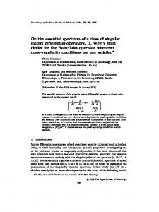
Fig. 1: Fdho as a function of x = E/ω for κ = λ/ω = 0.7, ∆ = µ/ω = 0, in the case when the spectrum of the Rabi model reduces to that of a displaced harmonic oscillator. In agreement with the exact analytic formula (17), the zeros of Fdho (x) satisfy xl = l − 0.49.

The function F (x) is different from the G-functions of Braak [8]. The latter have only been obtained in the case of the Rabi model by making explicit use of the parity symmetry. In contrast to Braak’s result [8], our F (x) can be straightforwardly defined for any model from R. The definition of F (x) does not require either a discrete symmetry or to solve the three-term difference equation (2) explicitly. All what is needed to determine F (x) is an explicit knowledge of the recurrence coefficients an and bn . This brings about a straightforward numerical implementation [10] and results in a great simplification in determining the spectrum. The proof of principle is demonstrated in fig. 1 in the case of exactly solvable displaced harmonic oscillator [1]. The ease in obtaining the spectrum is of importance regarding recent experimental advances in preparing (ultra)strongly interacting quantum systems [11–15], which can no longer be reliably described by the exactly solvable JC model [7], and wherein only the full quantum Rabi model can describe the observed physics. Proof of the main result. – In earlier studies [1, 4, 5, 8], largely motivated by the Frobenius method [16] of solving differential equations, the n = 0 part of the recurrence (2) was taken as an initial condition. Given the requirement of analyticity [c−k ≡ 0 for k > 1; cf. eq. (3)], the three-term recurrence (2) degenerates for n = 0 into an equation involving mere two terms and imposes that c1 /c0 = −a0 . (10)

• (ii) a minimal solution {mj }∞ j=0 . The respective solutions differ in the behavior cn+1 /cn in the limit n → ∞. The minimal solution guaranteed by the Perron-Kreuser theorem (Theorem 2.3 in ref. [3]) for models of the class R satisfies mn+1 b 1 ∼− τ →0 mn an

(n → ∞)

(11)

in virtue of (4) and τ ≥ 1/2 > 0. On substituting the minimal solution for the cn ’s in eq. (3), φ(z) automatically becomes an entire function. In what follows, the entire function generated by the minimal solution of the n ≥ 1 part of (2) will be denoted as φm (z). Now (11) presumes [up to the terms reducing to a O(1) term in (11)] an asymptotic behaviour mn ∼ k n /[Γ(n + 1)]τ

(12)

with k = −b/a. A sufficient condition for a minimal solution to generate φm (z) ∈ B can be read off from asymptotic properties of the generalized Mittag-Leffler function Eτ,γ (z) (cf. Sec. 3 of [17]), an entire function with the expansion coefficients 1/Γ(τ n + γ), where τ and γ are real constants. In brief φm (z) ∈ B if the leading-order decay of mn for n → ∞ is not slower than ∝ k n /Γ(τ n + γ), where k is a constant and τ > 1/2. For τ = 1/2 the√otherwise unrestricted constant k has to satisfy |k| < / 2. Up to an irrelevant proportionality constant, [Γ(n + 1)]τ ≈ (n)τ /2 (τ τ )n Γ(τ n + 1).

(13)

Therefore, when Γ(τ n + 1) had been substituted by [Γ(n + 1)]τ in Eτ,γ (z), one would have arrived at substantially the τ same conclusions, but √ with k replaced by kτ . For τ = 1/2 the latter yields k/ 2, and hence the sufficient condition |k| < 1 for φm (z) to belong to B (cf. eq. (1.4) of ref. [2]). Now it is important to realize that only the ratios of subsequent terms mn+1 /mn of the minimal solution are By solving the recurrence upwardly, one as a rule arrives related to infinite continued fractions (cf. Theorem 1.1 at the expansion coefficients of singular functions outside due to Pincherle in ref. [3]) the physical Bargmann Hilbert space B [1,4,16]. Only at a particular discrete set of parameter values that correspond −bn+1 bn+2 bn+3 mn+1 = ··· (14) rn = to the spectrum of a model the functions would belong to mn an+1 − an+2 − an+3 − p-2

On the spectrum of a class of quantum models Any minimal solution is, up to a multiplication by a constant, unique [3]. This has two immediate consequences. First, φm (z) is, up to a multiplication constant, unique. Second, the ratio r0 = m1 /m0 of the first two terms of a given minimal solution is unambiguously fixed. Note that the ratio r0 = m1 /m0 involves m0 , although it takes into account the recurrence (2) only for n ≥ 1 [3]. The remaining n = 0 part of the recurrence (2) imposes another condition [cf. eq. (10)] on the ratio r0 = m1 /m0 . The condition (10) can be translated into the boundary condition on the logarithmic derivative of φm (z), r0 =

φ′m (0) = −a0 . φm (0)

(15)

Obviously, one has r0 6= −a0 in general. As a rule it is impossible to find a minimal solution satisfying an arbitrarily prescribed initial condition on the ratio m1 /m0 of its first two terms. (This point was not made clear by either Schweber [1] or later on by Braak [8].) If one defines the function F = a0 + r0 , with r0 given by the continued fraction in (14), the zeros of F would correspond to those points in a parameter space where the condition (15) is satisfied. Then the coefficients of φm (z) ∈ B satisfy the recurrence (2) including n = 0, and φm (z) belongs to the spectrum. Analogous to the Schr¨odinger equation, the boundary condition (15) enforces quantization of energy levels. The rest of the proof follows upon an application of the Euler theorem, which transforms the continued fraction defining r0 in eq. (14) into an infinite series (cf. eqs. (4.4)-(4.5) on p. 43 of [3] forming the basis of the “third” method of Gautschi [3] at the special case of his N = 0 that is also used in our numerical implementation [10]). The latter leads directly to eqs. (8) and (9) for F [9]. The series in (8) converges whenever the continued fraction in (14) converges for n = 0, which occurs if and only if φm (0) = m0 6= 0 (cf. Theorem 1.1 due to Pincherle in ref. [3]). Illustration of some basic properties. – In the case of a displaced harmonic oscillator, which is the special ˆ R in (7) for µ = 0, the recurrence (2) becomes case of H (cf. eq. (A.17) of ref. [1]) 1 n−x cn + cn−1 = 0, cn+1 + (n + 1)κ n+1

cn = κα−n L(α−n) (κ2 ), n

(17)

where l ∈ N is a nonnegative integer (including zero). As demonstrated in fig. 1, Fdho (x) defined by eqs. (8) and (9) displays for ω = 1 and κ = 0.7 a series of discontinuous branches extending monotonically between −∞ and +∞, which intersect the x-axis at xl = l − 0.49, l = 0, 1, . . ..

(18)

where α = x + κ2 and Lβn are associated Laguerre polynomials [19] (note different sign of κ compared to eq. (2.16) of Schweber [1]). The substitution (18) transforms (16) into a 3-point rule that is identically satisfied by the associated Laguerre polynomials [19]. The Rodrigues formula [19]
z −α ez dn L(α) e−z z n+α (19) n (z) = n n! dz (α)

(α)

implies L0 (z) = 1, L1 (z) = −z + 1 + α, and in virtue of (18) (α)

c0

= κα L0 (κ2 ) = κα ,

c1

= κα−1 L1

(α−1)

(κ2 ) = κα−1 x.

(20)

Thus c1 /c0 = x/κ, which is exactly the n = 0 part of (16). In view of the asymptotic [19]   (α−n) z α , (n → ∞) (21) Ln (z) ≈ e n where the (generalized) binomial coefficients   α(α − 1)(α − 2) · · · (α − k + 1) α := , k k!

(22)

one finds from (18) 1α−n 1 cn+1 ∼ →− , cn κ n+1 κ

(16)

where dimensionless parameter κ = λ/ω reflects the coupling strength and x = ǫ = E/ω is a dimensionless energy parameter. Energy levels satisfy [1] ǫl = El /ω = l − κ2 ,

The zeros correspond exactly to the position of the energy levels (17). In the present example one can also explicitly illustrate that the difference equation (2) with the condition (10) imposed as an initial condition of the recurrence, and then solved upwardly, always possesses a solution. Obviously, such a solution would be generally a dominant solution. Consequently, the function φ(z) defined by power series expansion (3) with the expansion coefficients {dj }∞ j=0 would exhibit (typically branch-cut [1]) singularities in the z-complex plane and would not belong to B. Indeed, the recurrence (16) is solved for n ≥ 0 with

(n → ∞)

(23)

whenever α 6∈ N. Therefore, unless α is a nonnegative integer, the solution of eq. (18) is the dominant solution, the power series solution (3) has only a finite radius of convergence and thus does not belong to B. Only if the condition (17) is satisfied, α = x + κ2 is an integer, the dominant solution changes smoothly into the minimal solution of the recurrence (18), and the corresponding Fdho vanishes. In the case of the Rabi model, the recurrence (2) becomes 1 fn (x) cn + cn−1 = 0, (24) cn+1 − (n + 1) n+1

p-3

Alexander Moroz where fn (x) is given by   ∆2 1 n−x− , fn (x) = 2κ + 2κ n−x

(25)

is the familiar operator known to generate a continuous U (1) symmetry of the JC model [7, 8]. In contrast to ref. [8], our approach does not necessitate any active use of any underlying discrete symmetry. This has been demonstrated in a recent comment [9], where the regular spectrum of the Rabi model has been reproduced as zeros of a corresponding FRd (x) based on the recurrence (24). Obviously it was not possible then to determine what is the parity of a state corresponding to a given zero of FRd (x). Nevertheless, not only any discrete symmetry can be easily incorporated in our approach, this can be accomplished more straightforwardly and more easy than in the ˆR approach of Braak [8]. Indeed, the Rabi Hamiltonian H is an example of a general Fulton and Gouterman Hamiltonian of a two-level system [20]

κ = λ/ω, as in eq. (16), and dimensionless ∆ = µ/ω (cf. eq. (A8) of Schweber [1], which has mistyped sign in front of his bn−1 , and eqs. (4) and (5) of [8]). At first glance the recurrence (24) does not reduce to (16) for ∆ = 0 as one would expect from (7). The equivalence of eqs. (16) and (24) for ∆ = 0 is disguised by the fact that the recurrence (24) has been obtained after the unitary transformation of ˆ R in (7) induced by D = exp[κ(ˆ H a† − a ˆ)σ1 ] [1]. Thereby the dimensionless energy parameter x in eqs. (24), (25) is x = (E/ω) + κ2 . Both examples (16) and (24) represent the special Poincar´e case characterized in that the respective an and ˆ F G = A 1 + Bσ1 + Cσ3 , H (30) bn in (4) have finite limits a ¯ and ¯b = 0 [1,3,18]. The recurrences (16) and (24) correspond to the choice of δ = 0 and υ = −1 in (4), and hence τ = 1. They only differ in the with value of a ¯ = 1/κ in (16) and a ¯ = −1/(2κ) in (24), whereas A = ωˆ a† a ˆ, B = λ(ˆ a† + a ˆ), C = µ. (31) ¯b = 1 in both examples. Linearly independent solutions of (24) can be written for n ≫ 1 as The Fulton and Gouterman symmetry operation gˆ [20] is  realized by reflections 1/(nκn ), dominant νn = (26) nx κn /Γ(n + 1), minimal, a ˆ → −ˆ a, a ˆ† → −ˆ a† , (32) in agreement with (A.29a,b) of Schweber [1] and eq. (12) [note that nx leads to O(1) term in (11)]. In order to which leave the boson number operator a ˆ† a ˆ invariant. Beestablish asymptotic of φm (z) for z → ∞, one defines cause [ˆ g , A] = [ˆ g, C] = {ˆ g, B} = 0, gˆσ3 is the symmetry of ˆ R [20]. To any cyclic Z2 operator, such as gˆσ3 , one can ∞ H X χ(z) = νn z n , (27) associate a pair of projection operators n=0

where the minimal solution (26) has been substituted for νn . Obviously, φm (z) ∼ χ(z) for z → ∞. The asymptotic of χ(z) can be determined by the saddle point of the EulerMaclaurin integral representation of χ(z) [17, 21, 22]. For z → ∞ and | arg z| ≤ π/2, which comprises the positive real axis with the largest growth of χ(z), one finds a unique saddle point in the cut complex plane that completely governs the asymptotic behaviour of χ(z) [17, 21, 22],

P± =

1 (1 ± gˆσ3 ), 2

P±


2

= P ±.

(33)

However, because of gˆσ3 , the projectors P ± do not mix the upper and lower components of a wave function φ (conventional Pauli representation of σ1 and σ3 is assumed). In order to employ the Fulton and Gouterman reduction in the positive and negative parity spaces, wherein one component of φ is generated from the other by means of the χ(z) ∼ h(z, x) eκz+[x−(1/2)] ln[κz+x−(1/2)] + O(|z|p ), (28) operator gˆ, one is forced to work in a unitary equivalent single-mode spin-boson picture p where h(z, x) = κz + x − (1/2) and p is real constant ˆ R = ωˆ satisfying −1 < p < 0. As expected, χ(z) behaves essenH a† a ˆ + µσ1 + λσ3 (ˆ a† + a ˆ). (34) κz tially as e , because the asymptotic of the minimal soluby means of the unition (26) is only a slightly perturbed version of 1/Γ(n+ 1). The transformation is accomplished √ Consequently, φm (z) ∈ B for all model parameters. The tary operator U = (σ1 + σ3 )/ 2 = U −1 . The transformaleading order behaviour of the recurrence coefficients in tion interchanges the expressions for B and C in (31), reˆ R . Eqs. (4.12) (16) for n → ∞ resembles that of the Rabi model and the sulting in gˆσ1 becoming the symmetry of H above conclusions apply also to the case of the displaced and (4.13) of [20] then yield harmonic oscillator. [ωˆ a† a ˆ + λ(ˆ a† + a ˆ) ± µˆ g ]φ± = E ± φ± , (35) ˆR Discrete symmetries. – The Rabi Hamiltonian H [eq. (7)] is known to possess a discrete Z2 -symmetry cor- where the superscripts ± denote the positive and negative responding to the constant of motion, or parity, Pˆ = parity eigenstates of P ± [with σ3 being replaced by σ1 in ˆ [4, 8], where exp(iπ J) (33)]. Working in the Bargmann space, 1 (29) Jˆ = a ˆ† a ˆ + (1 + σ3 ) [ωz∂z + λ(z + ∂z ) ± µˆ g ]φ± = E ± φ± . (36) 2 p-4

On the spectrum of a class of quantum models

positive parity

positive parity

negative parity

negative parity

8

5

6

4

4 3

R

F (x)

2 0

2

-2

1

-4 0

-6 -8 -1

-1

0

1

2

3

4

5

0,0

0,1

0,2

0,3

0,4

x

Fig. 2: FR (x) for κ = 0.7, ∆ = 0.4, and ω = 1, i.e. the same parameters as in fig. 1 of ref. [8], shows zero at ≈ −0.707805 for a negative parity state and at ≈ −0.4270437 for a positive parity state. After addition of κ2 = 0.49 they correspond to the zeros at −0.217805 and 0.0629563, respectively, in fig. 1 of refs. [8, 9].

Fig. 3: Energy levels for κ = 0.7 and ω = 1 as a function of ∆ evolve from the doubly degenerate level corresponding to those of the displaced harmonic oscillator at ǫl = l − 0.49 to the parity eigenstates of the Rabi model.

functions G± (x) in the variable x = (E/ω) + κ2 [8],   ∞ X Eqs. (36) are equivalent to a coupled system of first-order ∆ κn . (39) G (x) = K (x) 1 ∓ ± n eqs. (10) of the supplement to [8]. In contrast to [8], x − n n=0 one does not need any ill motivated substitution to arrive at the symmetry resolved spectrum of thePRabi model. Here the coefficients Kn (x) were obtained recursively by ∞ n Assuming power series expansions φ± (z) = n=0 c± e difference equation (24) upwardly n z for solving the Poincar´ the positive and negative parity states, one arrives directly starting from the initial condition (10). Braak needed one at the following three-term recurrence page of arguments (between eq. (10) on p. 2 and the end of the first paragraph on p. 3 of the on-line supplement to 1 [8]) to arrive at his G± (x). The arguments involved an ill [n − x ± (−1)n ∆]c± c± n n+1 + κ(n + 1) motivated substitution and that a sufficient condition for 1 + c± = 0, (37) the vanishing of an analytic function G+ (x; z) (defined by n + 1 n−1 eq. (16) of his supplement) for all z ∈ C is if it vanishes at a single point z = 0. The argument is essential to ar± where x = E /ω and κ = λ/ω, as in eq. (16), and ∆ = rive at (39). However, as an example of any homogeneous µ/ω, as in eq. (24). In arriving at eqs. (37) we have polynomial shows, the argument is obviously invalid. One merely used that needs additionally that (d/dz)G± (x; z) = 0 at z = 0 [23]. ∞ At zeros of G± (x) the coefficients Kn ’s in (39) have to be X n gˆφ± (z) = φ± (−z) = (−1)n c± (38) the minimal solutions. The difficulty of calculating mininz . n=0 mal solutions can be illustrated by an attempt to calculate the Bessel functions of the first kind Jn (x) for fixed x = 1 ± Upon defining corresponding FR (x) by means of eqs. (8) by an upward three-term recurrence from the initial values and (9), one can not only recover the regular spectrum of J0 (x) and J1 (x). It turns out that all digits calculated in the Rabi, but also distinguish different parity eigenstates. single precision came out illusory already for n ≥ 7 (cf. This is demonstrated in fig. 2. Fig. 3 demonstrates that Table 1 of [3]). on setting ∆ = 0 the parity eigenvalues become doublyWe have advanced an alternative approach which does degenerate eigenvalues corresponding to those of a disnot require any explicit solution of any difference equation placed harmonic oscillator. That was to be expected, beand which applies to an entire class of models. A symmecause the three-term recurrence (37) then reduces to the try is not required to characterize a quantum model in three-term recurrence (16). terms of a suitable F (x). Contrary to ref. [8], F (x) can Discussion. – In his recent letter [8], Braak claimed be obtained directly from the recurrence coefficients charto solve the Rabi model analytically (see also Viewpoint acterizing an eigenvalue equation of a given model. In the by Solano [24]). He suggested that a regular spectrum of case of the Rabi model, nothing but the elementary relathe Rabi model was given by the zeros of transcendental tion (38) has been employed in arriving from (36) to (37), p-5

Alexander Moroz and the corresponding FR± (x) were unambiguously determined from (37) through eqs. (8) and (9). The resulting transcendental functions FR± (x) are different from G± (x) considered by Braak [8]. With the exception of the displaced harmonic oscillator and the JC model, the zeros of F (x) have to be still determined numerically. Therefore we disagree with Solano’s view [24] that a mere characterization of a model by a function such as G± (x) of ref. [8], or our F (x), is tantamount to solving the model analytically in a closed-form. Our results rejuvenate the Schweber quantization criterion r0 + a0 = 0 known in the case when r0 remained to be expressed in terms of continued fractions [e.g. eq. (14)] [1]. The Schweber criterion was deemed impractical and has not been employed to solve for the quantized energy levels of any quantum model [1, 4, 5, 8]. The criterion was either regarded to require a numerical diagonalization in a truncated Hilbert space (pp. 4-5 of the on-line Supplement to ref. [8]), or simply refuted as being identically valid irrespective of the value of an energy parameter x (see for instance p. 4 of the on-line Supplement to ref. [8]). With the help of the Euler theorem, which transforms the continued fractions into an infinite series, our approach turned the Schweber quantization criterion into an efficient computational tool. Our approach has been demonstrated on the examples of a displaced harmonic oscillator and the Rabi model. However, the outlined approach would work for any of the models of the class R. For instance, the JC model and the single-mode spin-boson form of a generalized Rabi model introduced in [8], HRθ = ωˆ a† a ˆ + λσ3 (ˆ a† + a ˆ) + θσ3 + µσ1 ,

(40)

where θ is a deformation parameter. Another example is a modified Rabi model with the interaction Hamiltonian ˆ int = i~λσ1 (ˆ H a† − a ˆ). The latter arises if the dipole interaction with a Fabry-P´erot cavity light mode is replaced by the interaction with a single-mode plane-wave field. We have characterized our class R of models implicitly in that their eigenvalue equation can be reduced to a difference equation (2) with its coefficients satisfying eq. (4). An interesting problem is to provide an explicit characterization of the models. Eventually note that whereas the condition τ ≥ 1/2 ensures φm (z) ∈ B, one needs only τ > 0 to define F (x) by eq. (8) if m0 6= 0. Conclusions. – A general formalism has been developed which allows to determine the spectrum of an entire class of quantum models as zeros of a corresponding transcendental function F (x). The function can be analytically determined as an infinite series defined solely in terms of recurrence coefficients. The class of quantum models comprises the displaced harmonic oscillator, the JaynesCummings (JC) model, the Rabi model, and a generalized Rabi model. Applications of the Rabi model range from quantum optics and magnetic resonance to solid state and molecular physics. The model plays a prominent role in

cavity QED and circuit QED, and can be experimentally realized in Cooper-pair boxes, flux q-bits, in Josephson junctions or using trapped ions, and is of importance for various approaches to quantum computing. Therefore, our results could have implications for further theoretical and experimental work that explores the interaction between light and matter, from weak to strong interactions. The ease in obtaining the spectrum is of importance regarding recent experimental advances in preparing (ultra)strongly interacting quantum systems, which can no longer be reliably described by the exactly solvable JC model. The relevant computer code has been made freely available online [10]. ∗∗∗ I thank Professor Gautschi for a discussion. Continuous support of MAKM is largely acknowledged. REFERENCES [1] [2] [3] [4] [5] [6] [7] [8] [9] [10] [11]

[12]

[13] [14] [15] [16] [17] [18]

[19] [20] [21] [22] [23] [24]

p-6

Schweber S., Ann. Phys. (N.Y.), 41 (1967) 205. Bargmann V., Comm. Pure Appl. Math., 14 (1961) 187. Gautschi W., SIAM Review, 9 (1967) 24. Kus M., J. Math. Phys., 26 (1985) 2792. Kus M. and Lewenstein M., J. Phys. A: Math. Gen., 19 (1986) 305. Rabi I. I., Phys. Rev., 49 (1936) 324. Jaynes E. T. and Cummings F. W., Proc. IEEE, 51 (1963) 89. Braak D., Phys. Rev. Lett., 107 (2011) 100401. Moroz A., arXiv:1205.3139. The source code can be freely downloaded from http://www.wave-scattering.com/rabi.html. Bourassa J., Gambetta J. M., Abdumalikov A. A., Jr., Astafiev O., Nakamura Y. and Blais A., Phys. Rev. A, 80 (2009) 032109. Forn-D´ıaz P., Lisenfeld J., Marcos D., Garc´ıa-Ripoll J. J., Solano E., Harmans C. J. P. M. and Mooij J. E., Phys. Rev. Lett., 105 (2010) 237001. Niemczyk T. et al, Nature Phys., 6 (2010) 772. Schwartz T., Hutchison J. A., Genet C. and Ebbesen T. W., Phys. Rev. Lett., 106 (2011) 196405. Crespi A., Longhi S. and Osellame R., Phys. Rev. Lett., 108 (2012) 163601. http://en.wikipedia.org/wiki/Frobenius_method Moroz A., Czech. J. Phys. B, 40 (1990) 705. In the Poincar´e case the limits of cn+1 /cn for n → ∞ are readily determined by the roots of the characteristic polynomial Φ(t) = t2 + a ¯t + ¯b. http://en.wikipedia.org/wiki/Laguerre_polynomials Fulton R. L. and Gouterman M., J. Chem. Phys., 35 (1961) 1059. Fedoriuk M. V., Asymptotic estimates: Integrals and series (in Russian) (Nauka, Moscow) 1987. Evgrafov M. A., Asymptotic estimates and entire functions (in Russian) (Nauka, Moscow) 1979. Maciejewski A. J., Przybylska M. and Stachowiak T., arXiv:1210.1130 Solano E., Physics, 4 (2011) 68.