supply sources mix consists of 45.5% surface water, 45.5% ground- water, and 9% ... Pasco, and Pinellas Counties, and the cities of New Port Richey,. Tampa, and St. ..... the approach used the power of both AMPL and Matlab to cut.
On the Use of System Performance Metrics for Assessing the Value of Incremental Water-Use Permits
Downloaded from ascelibrary.org by Tirusew Asefa on 06/18/14. Copyright ASCE. For personal use only; all rights reserved.
Tirusew Asefa, Ph.D., P.E., M.ASCE 1; Nisai Wanakule, Ph.D., P.E., M.ASCE 2; Alison Adams, Ph.D., P.E., M.ASCE 3; Jeff Shelby 4; and John Clayton, Ph.D., P.E., M.ASCE 5
Abstract: A novel approach on quantifying the value of an incremental surface water–use permit in an integrated water resources system consisting of groundwater, surface water, off-stream reservoir, and desalinated seawater sources is presented. First, a stochastic framework that accounts for demand uncertainties and variations in climatic parameters was used to generate regional demand and supply realizations. Second, a linked optimization-simulation model was used to navigate through complex system constraints and sustainable operational constraints. The resulting decision variables were then used to calculate system performance metrics, demonstrating the benefit of an increase in surface-water withdrawals at high flows. The Monte Carlo–based model took advantage of distributed computing capabilities on a private cloud computing system to significantly reduce the total run time. The model codes were developed in two different software environments, executed on different platforms, in which information was exchanged through an inter-process communication (IPC) protocol. The major contribution of this research is toward the practical use of stochastic-based integrated surface/groundwater–use permit application for a complex water resources system. The approach is demonstrated using Tampa Bay Water’s integrated water resources system. DOI: 10.1061/(ASCE)WR.1943-5452.0000388. © 2014 American Society of Civil Engineers. Author keywords: Performance metric; Water-use permit; Distributed computing; Integrated water resources system.
Background In 2005 (the most recent year for available data), the United States used an estimated 55.26 mm3 =day of water for public supply consumption, of which 8.33 mm3 =day came from groundwater sources (Kenny et al. 2009). In Florida, 86.7% of the public water supply (1.26 mm3 =day) was from groundwater and 13.3% from surface-water withdrawals. In the past decade, there has been a tangible shift from groundwater-only-type sources of supply to alternative source systems because of tremendous environmental stress that heavy groundwater use has caused. For example, at Tampa Bay Water, the largest wholesale water supplier in the Southeastern United States with a customer base of over 2.3 million, the 2011 supply sources mix consists of 45.5% surface water, 45.5% groundwater, and 9% desalinated seawater. This is very different from 100% groundwater in 1998 and 74.4% groundwater as recently as 2007. The transition to incrementally higher surface-water supply brings uncertainties in quantification of future supply availability that were not seen when all of the supply came from groundwater. As a result, a more complex modeling approach of supply 1
Senior Water Resources Engineer, Tampa Bay Water, 2575 Enterprise Rd., Clearwater, FL 33763 (corresponding author). E-mail: tasefa@ tampabaywater.org 2 Modeling Supervisor, Tampa Bay Water, 2575 Enterprise Rd., Clearwater, FL 33763. 3 Senior Manager, Tampa Bay Water, 2575 Enterprise Rd., Clearwater, FL 33763. 4 Software Architect, Tampa Bay Water, 2575 Enterprise Rd., Clearwater, FL 33763. 5 Associate, Hazen and Sawyer, 5775 Peachtree-Dunwoody Rd., Suite D-520, Atlanta, GA 30342. Note. This manuscript was submitted on March 20, 2012; approved on July 1, 2013; published online on July 4, 2013. Discussion period open until September 4, 2014; separate discussions must be submitted for individual papers. This paper is part of the Journal of Water Resources Planning and Management, © ASCE, ISSN 0733-9496/04014012(9)/$25.00. © ASCE
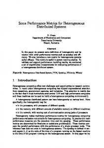
and demand that accounts for a variety of uncertainties in inputs, a model (because of uncertainty in the rainfall/runoff process), and climate variability in an integrated fashion are needed. Traditionally, water use–permit issues have been analyzed separately by supply sources, e.g., surface or groundwater. When more than one supply source is used, it is usually in a deterministic form without accounting for uncertainties, or only one of many future scenarios is considered. An integrated Monte Carlo–based optimization-simulation approach is demonstrated in this paper. Tampa Bay Water has an unequivocal obligation to meet the region’s water demand now and in the future. It provides potable water to its member governments consisting of Hillsborough, Pasco, and Pinellas Counties, and the cities of New Port Richey, Tampa, and St. Petersburg, using a complex distribution system of over 420 km of raw and finished water pipelines to 21 points of delivery. Over the last decade, the average annual delivery ranged between 870 and 1,000 m3 =day. The agency’s regional system includes (1) 13 wellfields consisting of 177 production wells, (2) six groundwater-treatment facilities, and (3) a 110-m3 =day seawater desalination plant, the largest in North America. The surface water system includes a 59-mm3 capacity off-stream reservoir, a 450-m3 = day surface water–treatment plant (SWTP), and two surface-water withdrawal facilities (the Alafia River and the Hillsborough River/ Tampa Bypass Canal system). The agency operates under three groundwater-use permits, of which the largest is the consolidated water–use permit (CWUP), which limits pumpage from 11 wellfields based on a 12-month moving average of 338 m3 =day. The agency also operates under two surface water–withdrawal permits that are subject to flow conditions and minimum flow requirements set by the Southwest Florida Water Management District (SWFMD), a regional authority. Fig. 1 schematically shows the surface water systems of Tampa Bay Water. The Hillsborough River flows into the Hillsborough River reservoir, from which the city of Tampa (COT) uses for its water supply. When there is sufficient flow over the Hillsborough River Dam
04014012-1
J. Water Resour. Plann. Manage. 2014.140.
J. Water Resour. Plann. Manage.
Downloaded from ascelibrary.org by Tirusew Asefa on 06/18/14. Copyright ASCE. For personal use only; all rights reserved.
Fig. 1. Surface water systems of Tampa Bay Water: Tampa Bypass Canal (TBC) and Alafia River
(HRD), Tampa Bay Water may divert water through structure S161 into the middle pool (MP) and then to the lower pool (LP) so that it can be used to send water directly to an SWTP or to be stored at an off-site reservoir. In case there is excess flow or flooding events, water is released through structure S160 into Tampa Bay. Surface-water withdrawal from Alafia River is used to either send water to an SWTP or to the reservoir. Both of these surface-water withdrawals are governed by the permit rules shown in Fig. 2. The current Alafia River withdrawal permit is set at 10%, even though in the past, Tampa Bay Water has been granted a 19% withdrawal on an emergency basis. Consequently, Tampa Bay Water filed a permit application based on the 19% withdrawal rate, to which SWFMD inquired: “Please provide an assessment of the reliability of Tampa Bay Water’s existing regional water supply system and the increase in reliability realized if the allowable flow available above minimum thresholds is increased from 10 percent of flows to 19 percent of flows,” (SWFMD 2010). The objective of the study is to assess the changes in performance of the overall system as a result of changes in Alafia River withdrawal rules. To this end, a variety of system performance metrics are used to assess the difference between 10 and 19% withdrawal permits.
system is in a satisfactory state (S) compared with the total simulation length (T). As such, it does not evaluate other statistics of unsatisfactory states (e.g., mean, variance, or return periods of the unsatisfactory states). Let X tðiÞ ; t ¼ 1; : : : ; T be a simulated time series of a parameter of interest, such as supply sources, which is used as an indicator of a system’s performance when compared with a criterion, CtðiÞ , such as system demand for the ith realization. A realization is defined as one possible future scenario of a unique combination of demand and supply distributions having a length of T years. The comparison would then indicate the system as being in either satisfactory, S, or unsatisfactory, states. Defining a state variable Z, where IfX tðiÞ ∈ S; ZtðiÞ ¼ 1 else X tðiÞ ∈ U the ith reliability is defined as CRðiÞ ¼
PT
t¼1
and
ZtðiÞ ¼ 0
ZtðiÞ
ð1Þ T Eq. (1) provides the distribution of time-based reliability across realizations. Realizations are generated to account for uncertainties in both demand and supply of the system. Resilience
Performance Metrics Some of the most widely used water resource–performance metrics are those consisting of reliability, resilience, and vulnerability measures (Hashimoto et al. 1982; McMohan et al. 2005). Each is described subsequently. Reliability Reliability measures the frequency or probability of a system’s success by simply counting the time (i.e., number of days) that the © ASCE
Resilience measures how quickly, on average, a system rebounds to a satisfactory state once it is in an unsatisfactory state (Hashimoto et al. 1982). Examples of how resiliency is applied are seen in a wide variety of applied sciences from material science to environmental systems (Wang and Blackmore 2009). In material science, resilience is the capacity of a material to absorb energy when it deforms elastically, and then upon unloading to have this energy recovered. There is no permanent deformation, and the material returns back to where it was. Let W tðiÞ be an indicator of transition from unsatisfactory to satisfactory state of the ith realization such that
04014012-2
J. Water Resour. Plann. Manage. 2014.140.
J. Water Resour. Plann. Manage.
S161 Diversion/Middle Pool Withdrawal off of Hillsborough River Criterion flow: total of measured previous-day flow over/through Hillsborough River Dam (HDR) and previous-day S161 diversion: Criterion flow, Mgd Permitted S161 Diversion/MP Withdrawal, Mgd
0 – 65 0
65 - 108.3 0-43.3
108.3 – 485 43.3 – 194
> 485 194
Downloaded from ascelibrary.org by Tirusew Asefa on 06/18/14. Copyright ASCE. For personal use only; all rights reserved.
Also limited by current-day (instantaneous) HRD flow to disallow withdrawals that would take HRD flow below 65 Mgd: Permitted S161 diversion and MPWD = lesser of permit based on previous-day total and instantaneous HRD flow minus 65 Mgd
Lower Pool Permitted Withdrawal 100% of any same-day measured Lower Pool volume over 9 ft elevation No minimum flow requirement over S160 259 Mgd maximum permitted withdrawal
Alafia Proposed Permitted Withdrawal Criterion flow: previous-day Alafia flow at Lithia Gauge x 1.117 + historical daily average flows on day t of the year at Lithia Springs + historical daily average flows on day t of the year at Buckhorn Springs + historical daily average Mosaic withdrawal on day t of the year Criterion flow, Mgd Permitted Alafia Withdrawal, Mgd
0 – 82.73 0
82.73 – 95.65 0-12.93
95.65 – 368.72 13.11 – 65
> 368.72 65
Fig. 2. Water-use permits for Tampa Bay Water
� W tðiÞ ¼
1 0;
if X tðiÞ U and otherwise
X tþ1ðiÞ ∈ S
Then the ith realization resilience is given by PT−1 t¼1 W tðiÞ P CRSðiÞ ¼ T − Tt¼1 ZtðiÞ
ð2Þ
ð3Þ
As shown in Eq. (3), resilience accounts for the number of rebounds (transitions from U to S state) as a fraction of total unsatisfactory days. Expressed as a percentage, the value of resilience ranges from 0 to 100. For a given realization, hence hydrology and demand, if the system goes into an unsatisfactory state and never recovers, its resiliency is zero. An example of this is when high demand overwhelms supply sources. In contrast, there are two cases for resilience of 100: (1) given stress (demand)—if the system never goes into an unsatisfactory state, its resiliency is assumed to be 100, and (2) if the system always recovers from an unsatisfactory state in the following time step, its resiliency is 100. Examples of both cases are presented in subsequent sections. Another useful way of expressing resilience is as the expected length of time, e.g., days or months, for which the system remains in an unsatisfactory state once it is in an unsatisfactory state. Both definitions describe an average system response. Sometimes, it is important to look at the statistics of different durations of unsatisfactory states. For example, one may want to know how frequently 90-day continuous unsatisfactory state occurs. Vulnerability
state of time step of one or more. Vulnerability measures the expected values of deficits (demand/supply), if they were to occur. There are a number of ways to define vulnerability in literature: (1) the average (over all events) of the maximum deficit of unsatisfactory events (Hashimoto et al. 1982); (2) the average deficit over a continuous unsatisfactory duration (Loucks 1997; Sandoval-Solis et al. 2011); (3) the probability of exceeding a certain deficit threshold (Mendoza et al. 1997); (4) the single max deficit of the time series (Fowler et al. 2003); or (5) the return period of a certain level of cumulative deficit (Asefa et al. 2014). Furthermore, a distinction is made here depending on (1) whether the metric is aggregated based on all events in the simulation, which is the case when only a single time series is used to define the metric (Hashimoto et al. 1982), (2) whether the parameter is estimated over all events and realizations (McMohan et al. 2005), or (3) whether the metric is estimated for each realization and looks at the population of the metrics across realizations, as used in this study. This approach allows one to see vulnerability as a function of different percentiles of demand and supply pairs; thus, it is possible to quantify, given hydrology, the level of vulnerability that the system faces as the stress (demand) on the system increases. Cases in which a system would require a capital improvement program as a consequence of exhausting current supply sources (not a topic of this paper) is a natural result of this type of approach. Vulnerability could also look at not only the cumulative deficit (extent vulnerability), but also on extreme unsatisfactory durations (Loucks 1997). In this study, two types of extent vulnerabilities are defined based on cumulative deficit �X � CVðiÞ ¼ max C − X tðiÞ ; j ¼ 1; : : : ; N ð4Þ
Both reliability and resilience measure the average success rate or how quickly the system rebounds when faced with adversity, without actually looking at the consequence of those unsatisfactory events. In this paper an event is defined as a continuous unsatisfactory © ASCE
t∈J j ðiÞ
CVðiÞ ¼ median
04014012-3
J. Water Resour. Plann. Manage. 2014.140.
�X t∈J jðiÞ
� C − X tðiÞ ; j ¼ 1; : : : ; N
ð5Þ
J. Water Resour. Plann. Manage.
where J jðiÞ ; : : : ; J NðiÞ = periods of unsatisfactory states for the ith realization. Eq. (4) represents the most extreme vulnerability case as it looks at the maximum cumulative deficit over an event for a given realization, and Eq. (5) gives the most likely vulnerability based on sample distributions of vulnerabilities rather than the maximum event in a realization.
Modeling Approach
reservoir storage level are defined as starting when reservoir level drops below 26 m and continuing until the level recovers above 30.5 m. This criterion also triggers what is known as Level IV in the Tampa Bay Water Shortage Mitigation Plan (WSMP), a drought plan for the region. WSMP levels were developed to define different levels of drought and accompanying outdoor water-use restrictions. For the second criterion, wellfield pumpage is the total of 11 wellfields under a consolidated water-use permit (CWUP). Behavior of these indicators is simulated and the results are analyzed against these criteria.
Downloaded from ascelibrary.org by Tirusew Asefa on 06/18/14. Copyright ASCE. For personal use only; all rights reserved.
Performance Indicators Indicators of system performance are needed before quantifying the metrics of system performance. These indicators diagnose the system being in a satisfactory or unsatisfactory state. Two indicators were evaluated for Tampa Bay Water’s regional system: (1) reservoir stage level and (2) exceedance of a 12-month running consolidated wellfield target of 338 M3 =day. Unsatisfactory states for
Demand Simulation The probabilistic demands for the year 2030 were used to assess the benefit to be gained from an increase in the percent of water withdrawn from the Alafia River, above minimum flow thresholds at high flow conditions. First, a projection and/or assumption on socioeconomic growth and policy condition for each of Tampa
Fig. 3. Implementation of distributed operations model system © ASCE
04014012-4
J. Water Resour. Plann. Manage. 2014.140.
J. Water Resour. Plann. Manage.
necessary simulations to 334 while maintaining the integrity of the simulation results statistics. An LHS is a multivariate stratified sampling technique that divides the random space into, in this case, 334 by 334 grids of Latin squares, each with equal probability. A square is then randomly chosen such that there would be only one square per row or column. Additional information on the LHS method can be found in Iman and Conover (1982). Two independent random variables, one in the form of annual total rainfall of the watershed representing the supply side ensemble variability, and a socioeconomic factor representing the demand side, were used as the basis for the LHS sampling. The analysis indicates that 334 realizations were adequate to represent variability in both supply and demand simulations (Adams, Alafia water use permit technical report, unpublished report, 2012).
Systems and Hydrological Models Implementation
Asefa et al. (2014) presents a detailed exposition of all of the models that are used in this study. The steps needed to arrive at the decision variables that are used to define satisfactory and unsatisfactory states are (1) monthly-scale seasonal Markov mixture (SMM) models, to simulate rainfall using a historical record of over 100 years (these were used to drive a rainfall/runoff model); (2) a multivariate seasonal auto regressive with eXogenous (MSARX) variable model, to simulate stream flows at three locations (Alafia River, Hillsborough River, and Tampa Bypass Canal); and (3) a multivariate, nonparametric disaggregation (MND) model, to disaggregate the monthly simulations into daily traces because operational models that also include surface water–use permits are on a daily time scale (Clayton et al. 2010).
Fig. 3 shows a schematic for a distributed optimization-simulation modeling system. The following two sets of programs were employed: 1. An algorithm developed using a modeling language for mathematical programing (AMPL) (see, e.g., Fourer et al. 2003) that solves the pipe-flow problem as an integer optimization case, encoding complex systems constraints and operational rules including bidirectional flows, head and temperaturedependent withdrawals, seasonal operations, and prescribed operating rules. The program was implemented on a private cloud computing system powered by an HP Proliant DL580 G7 with four 10-core CPUs, 512 GB of RAM, and nearly 1.6 terabytes of hard-drive space dedicated for virtual memory, reconfigured to allow up to 32 realizations to run simultaneously. 2. A simulation model based on the Matlab Distributed Computing (Math Works 2011) system over a cluster of 52 quad-core ProLiant BL460c G1 computers that communicated with the AMPL program at daily time steps. Because both programs reside on different platforms on a network, a series of inter process communication (IPC) procedure calls were used to process data back and forth between the two. In doing so,
Monte Carlo Sampling A thousand realizations, each representing the supply and demand side, were first generated. There are 1 million combinations, if one were to cover all possibilities. The initial investigation revealed that at least one third of the realization (in the order of 300) was necessary to make the problem computationally tractable without compromising the quality of the results. A Latin hypercube sampling (LHS) technique was then employed to reduce the number of 100 Alafia 10%
90
Alafia 19%
12
80
Difference in Reliability, (%)
70 60
Reliability
Downloaded from ascelibrary.org by Tirusew Asefa on 06/18/14. Copyright ASCE. For personal use only; all rights reserved.
Bay Water’s demand service area was generated using data from a variety of sources such as American Community Survey, Moody’s Analytics, the Florida Department of Transportation, and other planning agencies. Then, uncertainty around point projections was stochastically simulated using historical data and a multivariate, nonparametric resampling framework. Finally, each socioeconomic ensemble was paired with an ensemble simulation of weather variables constituting the forecasted demand time series for the service area. More on the approach can be found in Hazen and Sawyer (Tampa Bay Water’s revised probabilistic demand forecasting procedure and base-year 2010 probabilistic demand forecast, unpublished report, 2012).
50 40 30
10
8
6
4
20 2 10 0
0 70
(a)
75
80
85
90
Demand Percentile
95
50
100
55
(b)
60
65
70
75
80
85
90
95
100
Demand Percentile
Fig. 4. (a) Reliability for Alafia at 10 and 19%; (b) difference in reliability (solid line represents a localized average over five realizations) © ASCE
04014012-5
J. Water Resour. Plann. Manage. 2014.140.
J. Water Resour. Plann. Manage.
100
100 Alafia 10%
90
90
Alafia 19%
80
Difference in Resilience, (%)
80
Resilience, (%)
70 60 50 40 30
60 50 40 30 20
10
10
0 40
50
60
70
80
90
0
100
Percent Exceedance
(a)
40
50
60
(b)
70
80
90
100
Exceedance
Fig. 5. Resilience and difference in resilience
the approach used the power of both AMPL and Matlab to cut the simulation time required significantly, and to make the problem tractable. For example, 32 100-year-long demand-flow pairs (the maximum number of simulations on the HP) in the optimization-simulation daily model runs required 5 h to complete. Consequently, for the two scenarios that are reported in this paper, each of the 334 realizations took approximately 4.3 days, which would have been more than 4 years if simulated on a stand-alone standard computer.
Results and Discussion Reliability, Resilience, and Return Periods of Unsatisfactory States Fig. 4 shows the reliability for both Alafia 10 and 19% scenarios. Below 50% of demand there is no tangible difference between the two. As the system demand increases, the additional withdrawal for
19% scenario starts to make an impact. As shown in Fig. 4(b), the maximum reliability improvement found by averaging the top five realizations is approximately 10%, and the single maximum reliability improvement, which occurs at the 86th percentile demand, is 12%. After the 90th percentile demand, system reliability is very low in both scenarios. This is because, at that level of demand, system-supply sources are exhausted. From Fig. 5, the system has much higher resiliency with the Alafia River withdrawal rate at 19%. This indicates that when unsatisfactory states are encountered, the system rebounds quickly and returns to compliance. At the Alafia River withdrawal rate of 10%, 48% of the time the resilience is 100%, whereas at a 19% withdrawal rate this increases to 59%. The average improvement from Fig. 5(b) is 22.8%. Again, at demands greater than the 95th percentile, the system never rebounds from unsatisfactory states—even with the Alafia River withdrawal rate at 19%. This indicates that changes in infrastructure and new sources of supply would be required at this level of demand. 50
18 Alafia 10%
16
Alafia 10% Alafia 19%
45
Alafia 19%
40
14
Return Period, Year
Mean Unsat. Duration (Month)
Downloaded from ascelibrary.org by Tirusew Asefa on 06/18/14. Copyright ASCE. For personal use only; all rights reserved.
20
70
12 10 8 6
35 30 25 20 15 10
4
5
2 0 3
0 15
20
25
30
35
40
45
50
55
Percent Exceedance
Fig. 6. Mean unsatisfactory durations as a measure of resiliency © ASCE
6
9
Unsatisfactory Duration, month
60
Fig. 7. Return periods of a given unsatisfactory duration for 75–85th percentile of demand (shorter bars are Alafia 10%)
04014012-6
J. Water Resour. Plann. Manage. 2014.140.
J. Water Resour. Plann. Manage.
Ratio of Withdrawal vs. Availability/Reservoir Storage
Downloaded from ascelibrary.org by Tirusew Asefa on 06/18/14. Copyright ASCE. For personal use only; all rights reserved.
frequent, say, a 90-day-long unsatisfactory period is. Fig. 7 depicts unsatisfactory durations of a given length and their associated return periods for a 75–85 demand percentile. Basically, an increased Alafia River withdrawal extended the return periods of unsatisfactory durations of any length. For example, under the 19% scenario, a 3-month unsatisfactory duration comes once in 25 years, whereas it was once in 14 years under the 10% scenario—a 44% decrease in return period. Similar results are seen for unsatisfactory periods of higher durations. Fig. 8 shows the fraction of permitted withdrawal and reservoir storage levels for the 10 and 19% cases. A value of one indicates a complete use of (permitted) available withdrawal and full reservoir storage, respectively. At a 10% Alafia withdrawal rate, 74% of the time there is permitted withdrawal, whereas at 19% only 71% of the time. This indicates that 3% of the time, a 19% withdrawal scenario actually left behind permitted available water, whereas a 10% permit withdrawal did not. The reason is that the reservoir is full and the 19% scenario took advantage of the high quantity of available water at times of high flow to fill the reservoir.
1
0.8
0.6
0.4
Alafia 10% Res. at AR 10% Alafia 19%
0.2
Res. at AR 19%
0 0
10
20
30
40 50 60 70 Ensemble Percentile
80
90
100
Fig. 8. Fraction of Alafia River withdrawal and reservoir storage under two scenarios
Another way of evaluating the resiliency of a water resources system is by calculating the expected duration of the system being in an unsatisfactory state, on average (Hashimoto et al. 1982). Unlike the percentage approach described previously, this approach evaluates the duration (in days, months) of the system being in an unsatisfactory state. Fig. 6 illustrates these results. As shown in the figure, the 19% withdrawal rate significantly reduced the expected duration of being in unsatisfactory states at all exceedance levels. For example, there is a 50% chance of having unsatisfactory states in 4 or more months when the Alafia River withdrawal rate is 10%, but only a 39% chance of this occurrence under the 19% withdrawal rate scenario, reducing the risk significantly. As shown in Fig. 6, unsatisfactory states are either avoided when the Alafia River withdrawal rate is 19% (when mean unsatisfactory durations are zero under the 19%, but not under 10%, line crossing the x-axis) or the length is significantly reduced (the 10% line is above the 19% line). The expected duration approach of Fig. 6 looks at all unsatisfactory durations. Sometimes, one may want to know how
Vulnerability Most Extreme and Most Likely Vulnerability of Severity and Durations Severity is defined as the cumulative volume of a deficit and is determined by the volume of groundwater withdrawal from the consolidated wellfields over 338 m3 =day during an unsatisfactory event, to meet demand. In most cases there will be more than one event per realization. The most extreme severity case identifies the event with the highest cumulative volume deficit in a realization, whereas the most likely severity is the estimated median value for all unsatisfactory events identified in a realization. Fig. 9 compares the probability distribution of the most extreme event in terms of percent exceedance between Alafia River withdrawal rates of 10 and 19%. Similar plots (not shown) were also found for the most likely events. The distribution plots shown in Fig. 9 indicate a decrease in vulnerability of 11% of the cases because of the increase in the permitted withdrawal in the Alafia River from 10 to 19%, which is shown by the horizontal difference between the two distributions at their intersections with the x-axis. This indicates that the unsatisfactory states have been completely eliminated from 33
Fig. 9. Most extreme vulnerability of both duration and severity © ASCE
04014012-7
J. Water Resour. Plann. Manage. 2014.140.
J. Water Resour. Plann. Manage.
2
104
Duration Vulnerability (month)
10
Downloaded from ascelibrary.org by Tirusew Asefa on 06/18/14. Copyright ASCE. For personal use only; all rights reserved.
Extent Vulnerability (MG)
103
102
101
100 55
1
10
0
60
65
70
75
80
85
90
95
100
10
55
60
65
70
75
80
85
90
95
100
Percentile
Percentile
Fig. 10. Avoidable most extreme extent (MG) and duration (month) vulnerabilities
realizations because of the increase in Alafia River withdrawal rate. For the most extreme case, as shown in Fig. 9, the maximum improvement among these 33 realizations, signified by the vertical differences between the two distributions (red lines), is a reduction in severity of 5 mm3 and a reduction in duration of 8 months. These magnitudes of improvement are maintained for all realizations with percent exceedance of less than or equal to 46%. Similar results were also found for the most likely case, in which the maximum improvements in severity and duration are 0.74 mm3 and 4 months, respectively. Avoidable Vulnerability This section discusses the results of another approach for quantifying vulnerability. This approach evaluates when there is a CWUP violation under the 10% withdrawal scenario but not under the 19% withdrawal scenario. This analysis identifies the value of additional Alafia River withdrawal when it helps to avoid specific vulnerabilities and, hence, the term avoidable vulnerabilities. Fig. 10 shows that additional Alafia River withdrawals were able to eliminate significant shortage events both in terms of volume deficits and durations. This result holds when evaluating the most extreme events, based on the maximum of cumulative deficit for a realization, or the most likely scenario, based on the median of cumulative deficits. For example, using the most extreme case, at the 70th percentile, the use of an additional 2 mm3 of groundwater pumpage over the consolidated permit limit was avoided with the Alafia River withdrawal rate at 19%, and 0.5 mm3 of groundwater pumpage was avoided for the most likely case. The duration of the most-likely avoidable event is 2 months and the duration of the extreme event is 5 months.
Summary and Conclusions Traditionally, water-use permits are analyzed for a given source of supply, e.g., groundwater or surface water only. When more than one source is considered, it is usually done in a deterministic fashion because of the computational cost related with accounting for different sources of uncertainties. As an alternative, this paper presents a comprehensive system-performance evaluation technique to demonstrate the value of incremental surface-water © ASCE
withdrawal permits within a fairly complex integrated water resources system. It accounts for a variety of uncertainties in both demand and supply models using a Monte Carlo approach to generate equally likely future scenarios that are consistent with historical records. First, a probabilistic framework was used to simulate demand for the year 2030. Second, stream flows were simulated for 100 years, constituting the supply side. Operational models representing system constraints and operating rules were then used to find decision variables for which system performance metrics were evaluated. Using a sampling technique, 334 realizations of demand/ supply pairs out of a million possibilities were selected to make the computational requirement tractable. Three metrics—reliability, resilience, and vulnerability—were used to measure, respectively, the frequency or probability of success of the system, the speed with which the system recovers once in an unsatisfactory state, and the consequence of being in an unsatisfactory state. Unsatisfactory state conditions were defined as times when the system cannot meet demand without violating the groundwater-use permit. To this end, a 12-month running average of the consolidated wellfield pumpage permit was used to define the unsatisfactory states. In addition to the three most popular metrics, several statistics such as return periods of unsatisfactory state of a given duration, were also simulated, providing additional evidence of benefits realized from increasing the permitted withdrawals from the Alafia River to 19%. The models were implemented on a private cloud computing and distributed computing system that enabled the evaluation of a wide range of future scenarios without the constraints of computational requirement. The main outcomes are listed as follows: 1. There is a quantifiable difference between 10 and 19% Alafia River withdrawal permit limits in both the percentage of unsatisfactory months and reliability. Improvement in regional system reliability increases when the regional demand ranges between the 50th and 86th percentiles. Regional system reliability improved an average of 10.3%; the single largest improvement was 12%. 2. Tampa Bay Water’s regional system displays remarkable resiliency by quickly rebounding from unsatisfactory states when the Alafia River withdrawal rate was increased to 19%. An average of 22.8% improvement in the regional system’s resiliency was obtained from increasing the permitted withdrawal levels;
04014012-8
J. Water Resour. Plann. Manage. 2014.140.
J. Water Resour. Plann. Manage.
Downloaded from ascelibrary.org by Tirusew Asefa on 06/18/14. Copyright ASCE. For personal use only; all rights reserved.
3. The Alafia River withdrawal rate of 19% significantly reduces the mean length of unsatisfactory durations or results in avoiding unsatisfactory states. For example, the likelihood of a 4-month unsatisfactory duration was lowered from 50 to just 39%. In addition, at 35% exceedance level, 10-month-long unsatisfactory durations were reduced to 7 months; 4. The 19% Alafia River withdrawal rate decreased the vulnerability of the regional system and eliminated the risk of vulnerability for 10% of the total number of realizations. For the most extreme vulnerability case, improvement was 5 mm3 ; in contrast, for the most likely vulnerability condition the reduction was 0.75 mm3 . Durations of unsatisfactory events were improved by 4 months for the most likely event and 8 months for the most extreme event; 5. For avoidable vulnerability cases (in which there is violation of the consolidated permit at the Alafia River withdrawal rate at 10% but not at 19%), the improvements are, respectively, 2 mm3 and 0.5 mm3 for the most extreme and most likely vulnerability events. Durations of unsatisfactory events were improved by 2 months for the most likely event and 5 months for the most extreme event; and 6. Increased Alafia withdrawal resulted in an additional longterm reservoir yield of 5 mm3 . The expected long-term average withdrawal of water from the Alafia River under the 19% withdrawal scenario is 59,000 m3 =day, an increase of 23,000 m3 =day. Two major benefits of a Monte Carlo–based integrated water resources system analysis for looking at incremental water-use permits such as the one reported in this paper are (1) the results are robust in the sense that the approach explored a wide array of future scenarios accounting for uncertainties in both demand and supply sides; and (2) once the simulations are performed, a variety of system performance metrics can be defined, depending on one’s situation, without setting up a new optimization-simulation framework. This is possible because all system performance evaluations were done as post-processing.
Acknowledgments We thank two anonymous reviewers for their valuable contribution that improved the clarity and presentation of the current presentation.
© ASCE
References Asefa, T., Clayton, J., Adams, A., and Anderson, D. (2014). “Performance evaluation of a water resources system under varying climatic conditions: Reliability, resilience, vulnerability and beyond.” J. Hydrol., 508, 53–65. Clayton, J., Asefa, T., Adams, A., and Anderson, A. (2010). “Interannualto-daily multiscale stream flow models with climate effects to simulate surface water supply availability.” Innovations in watershed management under land use and climate change, ASCE, Reston, VA. Fourer, R., Gray, D. M., and Kernigham, B. W. (2003). AMPL: A modeling language for mathematical programming, 2nd Ed., Duxbury Press, Canada. Fowler, H. J., Kilsby, C. G., and O’Connell, P. E. (2003). “Modeling the impacts of climatic change and variability on the reliability, resilience, and vulnerability of a water resource system.” Water Resour. Res., 39(8), 1222. Hashimoto, T., Stedinger, J. R., and Loucks, D. P. (1982). “Reliability, resiliency, and vulnerability criteria for water resources system performance evaluation.” Water Resour. Res., 18(1), 14–20. Iman, R. L., and Conover, W. J. (1982). “Sensitivity analysis techniques: Self-teaching curriculum.” Nuclear Regulatory Commission Rep. NUREG/CR-2350, Technical Rep. SAND81-1978, Sandia National Laboratories, Albuquerque, NM. Kenny, J. F., Barber, N. L., Hutson, S. S., Linsey, K. S., Lovelace, J. K., and Maupin, M. A. (2009). “Estimated use of water in the United States in 2005.” U.S. Geological Survey Circular, 1344, USGS, 52. Loucks, D. P. (1997). “Quantifying trends in system sustainability.” Hydrol. Sci. J., 42(4), 513–530. Math Works. (2011). Matlab distributed computing server administrator’s guide, Natick, MA. McMohan, T. A., Adeloye, A. J., and Zhou, S. L. (2005). “Understanding performance measures of reservoirs.” J. Hydrol., 324(1–4), 359–382. Mendoza, V., Villanueva, E. E., and Adem, J. (1997). “Vulnerability of basins and watersheds in Mexico to global climate change.” Clim. Res., 9, 139–145. Sandoval-Solis, S., McKinney, D. C., and Loucks, D. P. (2011). “Sustainability index for water resources planning and management.” J. Water Resour. Plann. Manage., 10.1061/(ASCE)WR.1943-5452.0000134, 381–390. Southwest Florida Water Management District (SWFMD). (2010). “Request for additional information, water use permit (WUP) application No. 20011794.002.” Letter. Wang, C., and Blackmore, J. M. (2009). “Resilience concept for water resources system.” J. Water Resour. Plann. Manage., 10.1061/ (ASCE)0733-9496(2009)135:6(528), 528–536.
04014012-9
J. Water Resour. Plann. Manage. 2014.140.
J. Water Resour. Plann. Manage.