Gray, Sallis, and MacDonell have published multiple arti- cles on performing author identification using metrics [8] and case-based reasoning [22]. They have ...
On the Use of Discretized Source Code Metrics for Author Identification Maxim Shevertalov, Jay Kothari, Edward Stehle, and Spiros Mancoridis Department of Computer Science College of Engineering Drexel University 3141 Chestnut Street, Philadelphia, PA 19104, USA {max, jayk, evs23, spiros}@drexel.edu
Abstract Intellectual property infringement and plagiarism litigation involving source code would be more easily resolved using code authorship identification tools. Previous efforts in this area have demonstrated the potential of determining the authorship of a disputed piece of source code automatically. This was achieved by using source code metrics to build a database of developer profiles, thus characterizing a population of developers. These profiles were then used to determine the likelihood that the unidentified source code was authored by a given developer. In this paper we evaluate the effect of discretizing source code metrics for use in building developer profiles. It is well known that machine learning techniques perform better when using categorical variables as opposed to continuous ones. We present a genetic algorithm to discretize metrics to improve source code to author classification. We evaluate the approach with a case study involving 20 open source developers and over 750,000 lines of Java source code.
1 Introduction
Stylometry, the application of the study of linguistic style, is used to analyze the differences in the literary techniques of authors. Researchers have identified over 1,000 characteristics, or style markers, such as word length, to analyze literary works [3]. Linguistics investigators have used stylometry to distinguish the authorship of prose by capturing, examining, and comparing style markers [9]. Programming languages allow developers to express constructs and ideas in many ways. Differences in the way developers express their ideas can be captured in their programming styles, which in turn can be used for author identification.
In the context of programming languages, it has been shown that capturing style in source code can help in determining authorship. Previous work by Kothari et al. [13] examined source code as a text document and identified certain software developer peculiarities that persisted across different projects. Those styles were used to determine the authorship of disputed source code. Using text-based style markers such as line length and 4-character sequence distributions, they created developer profiles. These profiles were used to determine the authorship of source code with a success rate of over of 80% on a data set consisting of 24 open source projects. Author identification is useful in several real world applications, including criminal prosecution, corporate litigation, and plagiarism detection [14]. In this paper we focus on improving classification through the discretization of metrics used to construct developer profiles. Discretization is the process of partitioning a continuous space into discrete intervals. For example, some developers may use verbose language to comment their source code. Instead of quantifying the size of their comments based on the number of characters, words, or lines of text, one can create three categories, “short”, “medium”, and “long”. It is well known that a good discretization of data can improve the process of classification, not only in accuracy but in efficiency [7, 4]. The major challenge in discretization is how to determine the optimal number and intervals of the categories. Considering the previous example of describing the verbosity of comments in source code, it is a nontrivial task to determine how many categories of sizes there are, and how to define the intervals marking those categories. Finding how many intervals a continuous space can be divided into and what those intervals are, defines the optimization problem of discretization. In previous work [13, 14] to build developer profiles, the authors discretized metrics with small intervals. How-
Max Jay Ed
(a)
Max
Metric Extraction Tool
(b)
Jay Ed
(c)
Profile Database
(d)
Figure 1: Process of computing developer profiles; (a) Source code samples of known developers, (b) Metric extraction tool, (c) Metric evaluations per developer, (d) Database of profiles. ever, Shevertalov et al. [23] demonstrated that discretizing or “binning” large histograms into wider intervals when classifying packet streams proved to be more effective. Our work applies Shevertalov’s technique to solve the discretization problem as it applies to textual metrics in source code classification. The rest of this paper will first describe related work in extracting style from source code and discretization for use in machine learning in Section 2. Section 3 describes the process of metric extraction. The genetic algorithm developed to discretize those collected source code metrics is presented in Section 4. Section 5 demonstrates the effectiveness of our technique on a case study involving 20 open source developers and a code base of over 750,000 lines of code. We conclude with our analysis of the results as well as our plans for future work in Section 6.
2 Related Work A prominent example in the use of style markers to verify authorship is the Bacon/Shakespeare case [10]. It had been argued that Bacon authored works that have been credited to Shakespeare. This claim has since been disproved by forensic linguists using style markers. They debunked the claim that Bacon had written Shakespeare’s works by using word length frequencies and the most-frequent-word-occurrence statistics. Oman and Cook [17] performed preliminary investigations into style and its relationship with authorship. Spafford and Weeber discussed concepts such as structure and formatting analysis [24]. Sallis compared software authorship analysis to traditional text authorship analysis [20, 21]. Gray, Sallis, and MacDonell have published multiple articles on performing author identification using metrics [8] and case-based reasoning [22]. They have also investigated
author discrimination [16] via case-based reasoning and statistical methods. More recently, Ding and Samadzadeh used statistical analysis to create a fingerprint for Java author identification [6]. Their technique makes use of several dozen metrics (e.g., mean-function-name length), which they have statistically correlated to identify developers. Their metrics extraction technique is similar to our own. However, where they use mostly scalar metrics derived from the source code, such as means, our metrics are formulated as histogram distributions. Our conjecture is that this can capture more detail about a developer’s style, while still providing good identification capability. An issue in authorship identification, as well as other data mining problems, is the question of data selection. One can extract a multitude of metrics from source code. However, it is difficult to choose metrics that are useful. This problem is made more difficult by the fact that a different set of metrics may have better performance when considering different groups of authors and therefore needs to be recalculated for each sample set. Kothari et al. [13] used entropy filtering to select optimal metrics. Lange et al. [14] used a genetic algorithm to achieve similar results. Neither approaches to identify source code authorship used discretized metrics, which we will show improve the quality and performance of authorship identification techniques. Dougherty et al. [7] described the need for machine learning algorithms to have a discretized search space, and the effectiveness of various algorithms when provided categorical variables as opposed to continuous ones. For example, they demonstrate that the C4.5 induction algorithm [19] provides significantly better results when used with discretized input data. Dougherty et al. [7] also described range and frequencybased discretization techniques. These are simple and efficient unsupervised techniques that can produce good results under the proper circumstances. We discuss these ap-
proaches in greater detail in Section 5.
3 Metric Extraction
To determine the authorship of source code, we first extract developer profiles for a population of known developers. Figure 1 depicts the tool-chain for developing a database of profiles. The profiles describe inherent characteristics found in the source code of developers. We begin by obtaining several samples of code from a population of developers. We associate the samples to their respective developers and process them through one or more metric extraction tools. For each developer we obtain a list of metrics and their values. We store the metrics as developer profiles in a database for use in determining authors of unclassified source code. We store developers’ profiles as histogram distributions of the extracted metrics. For example, Figure 2 shows the histogram of the line lengths for a particular developer. The developer’s sample source code exhibits line lengths varying from zero characters to 120 characters, as can be see on the horizontal axis. The vertical axis indicates the normalized frequency of each line length. Previous work [13, 14] concentrated on creating a large space of metrics to use in classification. Our goal in this work was to evaluate the effect of discretization using a genetic algorithm. Therefore, we restricted our analysis to the four metrics that seemed to produce the best results as identified by previous work. Those metrics are: leading-spaces measure the number of whitespace used at the beginning of each line. The x-axis value represents the number of the given whitespace characters at the beginning of each line. leading-tab measure the number of tab characters used at the beginning of each line. The x-axis value represents the number of the given tab characters at the beginning of each line. line-len measures the length of each line of source code. The x-axis value represents the length of a given line. line-words measures how densely the developer packs code constructs on a single line of text. The x-axis value represents the number of words on a line.
4 Genetic Algorithm Previous work by Kyoung-jae Kim and Ingoo Han used a genetic algorithm (GA) to perform discretization as a part
of an artificial neural network (ANN) system to predict the stock price index [12]. They determined that an ANN had problems with large, noisy, and continuous data sets. Therefore, they implemented a GA to mitigate those limitations. They used the ANN as a part of the evaluation function to evolve good discretization policies. Guided by this approach, we coupled the GA used to discretize the data with our problem of classification. This section describes the elements of our genetic algorithm. Section 4.1 describes how we encode the discretization of a histogram representation of style metrics. Section 4.2 presents the evaluation function used in the GA process, and Section 4.3 discusses the GA’s breeding function.
4.1
Encoding
Candidate discretizations produced by the GA described in this section are encoded using a binary encoding scheme. A binary encoding scheme was chosen because it is generic and commonly used [25]. This encoding enables us to leverage previously established techniques.
To encode a discretization we need to identify break points, namely those values that begin and end each discrete interval. In our scheme, a 1 represents the location of a break point (Figure 3). For example, if the original histogram has the following five categories; 2,4,5,7, and 8, an encoding of 01001 corresponds to three buckets: x < 4, 4 ≤ x < 8, and 8 ≤ x.
4.2
Evaluation Function
Once we have an encoding, a GA requires an evaluation function to assess the fitness of a particular discretization. Four parameters must be computed to calculate the fitness: • number of misclassifications • number of bins • distance from each classified entity to the correct class • distance from each classified entity to the incorrect class
To train the GA, the set of training source files is divided into two separate sets, l1 and l2 . l1 is used as the learning set during and l2 as the corresponding test set. The set containing all of the source files of l1 and l2 is herein referred to as the training set. The evaluation function, illustrated in Figure 4, accepts a chromosome representing a discretization as input and
!#!+"
!#!*"
Normalized Count
!#!)"
!#!("
!#!'"
!#!&"
!#!%"
!#!$"
!" !"
$!"
%!"
&!"
'!"
(!"
)!"
*!"
+!"
,!"
$!!"
$$!"
$%!"
Line Size
Figure 2: Histogram of line sizes; Horizontal axis indicates the line size values, and vertical axis indicates the normalized frequency, or count, of that line size value for the particular developer. converts the undiscretized histograms into discretized histograms. The evaluation function then performs a nearest neighbor classification of the data. The learning set is used as expert knowledge by the classifier. To classify samples using the nearest neighbor classifier, a representative histogram for each class must be identified. One way to define a representative histogram is by computing the average among a set of histograms. However, when classifying styles, we found that including all of the learning histograms in the representative set produced better results. To determine the class of a sample from the test set, the Euclidean distance is calculated between it and each of the representative histograms in the learning set. The test sample is labeled as belonging to the same class as the representative histogram it is closest to. The performance of the nearest neighbor classifier is improved by either reducing the number of histograms in the learning set or, by reducing the number of categories in each histogram. Once classification is complete, a chromosome’s value is computed via:: E(x) =
1 100a + b + c − d
In the previous equation, a is the number of misclassifications, b is the number of bins in the discretized histograms, c is the average Euclidean distance between his-
tograms in the testing set and the closest histogram of the same class in the learning set, and d is the average Euclidean distance between histograms in the testing set and the closest histogram of a different class in the learning set. Since classification accuracy is the most important criterion, the number of misclassifications is weighted by an arbitrarily large factor in the equation; in this case, 100.
While keeping the number of misclassifications low is the top priority, we found that there were many different solutions with the same number of misclassifications. Therefore, other parameters were needed to further differentiate between candidate solutions.
The number of categories, the b parameter, was chosen to weigh the GA toward solutions with a smaller number of discrete intervals. The c and d parameters allow for small improvements. As the GA improves, the histograms in the testing set become more similar to histograms that belong to the same class and more dissimilar to histograms that belong to other classes. In early experiments the c and d parameters were ignored, thus leading to a quick convergence. By including these parameters, the GA converges slower, thus providing better results.
5
4 3 3
2
(a)
2
1 1
(b)
3
7
11
1
1
12
1
Learning
Testing
Unbinned Unbinned Histogram Unbinned Histogram Unbinned Histogram Unbinned Histogram Histogram
Unbinned Unbinned Histogram Unbinned Histogram Unbinned Histogram Unbinned Histogram Histogram
(a)
2
4
8
1
2
3
4
7
8
11
12
1
1
1
1
1
1
1
1 (b)
4
Binning
5 3 3
2
(c)
2
1
1
1 2 3 4 7 8 11 12
(d)
1 2 3 4 7 8 11 12
1
2
3
4
7
8
11
12
0
0
1
0
0
0
1
0
Testing
(c)
Unbinned Unbinned Histogram Unbinned Histogram Unbinned Histogram Binned Histogram Histogram
Unbinned Unbinned Histogram Unbinned Histogram Unbinned Histogram Binned Histogram Histogram
7
(d)
Nearest Neighbor Classification
11
(e)
Compute the Chromosome Value
6 4
Learning
1
4
(e)
1 11
Figure 3: Process demonstrating how the encoding can be used to combine multiple histograms. (a) presents the original histogram. (b) illustrates the encoding where it is composed of all 1’s and thus every bucket is its own bin. (c) demonstrates the results of the string encoding described in (b). (d) presents another sample encoding such that the result is three buckets: 0-2, 3-7, and 8-12. (e) demonstrates the results of the discretization described in (d).
Figure 4: Process used to compute the parameters of the evaluation function. (a) the training set is divided into two sets, learning and testing. (b) all histograms are discretized based on the chromosome being evaluated. (c) a discretized learning and testing sets of histograms are produced. (d) the testing set is classified using the nearest neighbor classifier. (e) the chromosome value is computed.
4.3
Breeding Function
After a population of chromosomes is evaluated, candidates are chosen to breed a new population. They are selected using the roulette selection algorithm, where the probability that a chromosome is chosen is weighted by its relative fitness. Once parents are chosen into the breeding pool, they are bred two at a time, at random, with replacement. The parents produce two children with a probability that is a configurable parameter in the implementation; it was set to 0.9 in in the case study. If they do not mate, the parents themselves are added to the next generation. In addition, the algorithm ensures that the next generation does not contain identical chromosomes. Using this restriction the GA is prevented from converging prematurely. A mutation operation is applied to the newly generated set of chromosomes. It is applied with a probability pm , corresponding to the current performance of the algorithm. When a mutation is applied, it changes a bit in the encoding from 1 to 0 with a probability pc , and from 0 to 1 with a probability 1 − pc . In this implementation, pc was set to be greater than 0.5 because we want the algorithm to spend more time exploring solutions with fewer categories (i.e., the algorithm is biased towards fewer discrete intervals). The encodings, represented as bit strings, can be very long containing mostly 0s. If the mutation function simply flips a random bit, it is more likely to change a 0 to a 1 and thus increase the number of discrete intervals. We found that by having greater control over which was modified, a 0 or a 1, we are able to emulate two different discretization operations, splitting a category, in the case of a 0 changing to a 1; and merging two categories, in the case of changing a 1 to a 0. This abstraction allows the algorithm to converge more quickly. The probability of mutation is set using a technique similar to simulated annealing [2]. As a generation improves, meaning that the average fitness of the population improves. The probability of mutation is decreased by a relatively large amount. If a generation does not improve, the probability of mutation is increased by a small amount, thus introducing more randomness to the search. In our case we used 0.001 as this probability. By allowing the algorithms to dynamically adjust the rate of mutation, it strikes a balance between exploring a local area of the search space, when mutation is low, and exploring the entire search space, when mutation is high. In our experiments this prevented the algorithm from converging too early by diversifying the pool of potential solutions.
5 Case Study To demonstrate the effectiveness of discretization via a GA, we applied our technique to a sample of opensource developers’ source code. The sample consisted of 60 projects by 20 developers (3 projects from each developer). Additionally we restricted the number of metrics to the following four, so that we could compare our discretized results with the undiscretized results of previous work: • • • •
leading-spaces leading-tabs line-length line-words
This case study uses source code from 20 developers found on the Sourceforge website [11]. We found the 20 most active developers who had at least three projects for which they were the sole developer. In total, the 60 projects constituted over 750,000 lines of code. Two projects were used for training, and the third for assessing the evolved solution. The genetic algorithm requires two sets to complete its work. The first is used to extract metrics and the second to assess candidate discretizations. The first hurdle we approached when attempting this case study was that the performance of the GA evaluation function was poor in terms of completion time, taking as long as 6 hours to evaluate a single population. To mitigate this problem, the algorithm was modified to use a smaller subset of source files to perform the evaluation. Five files from each developer were chosen at random during each evaluation step. This further evens out the playing field as the number of files was inconsistent across developers. They varied anywhere from 5-6 files to as much as 300 per project. By making this adjustment, the GA would not be biased toward any single developer and treat each one as having the same weight. In addition to comparing the GA-based discretization with non-discretized data, we wanted to evaluate it against two other discretization methods, range based and frequency based discretization [7]. Both of these are unsupervised methods that are relatively simple to implement and are not computationally expensive. Range based discretization creates N buckets of identical size, where N is specified by the user. The algorithm first determines the domain size of the undiscretized data, either through user input or by deriving it from the learning data set. It then divides the domain by N to determine the size of each interval. For example, assume a size distribution with the smallest observable size being 60, the largest being 1000, and a chosen N of 10. The new histogram will have 10 categories each of size (1000 − 60)/N = 94. Thus category 0 in the new histogram would contain the sum of categories 0 to 93 from the original histogram.
Unbinned
Unbinned
10
7
2
1
(a)
2
2
2
0
0
(a)
10 3
3
2
1
0
Distance: √3 Range
11
Frequency
Range
1
Frequency
9
9 1
(b)
(c) 10
9
1
(c)
10
8 2
Distance: √5
0
7
6
8
1
0
Distance: √105 10
(b) 10
0
8
0
0
1
Distance: √1
Figure 5: Range-based discretization improves results in this example. Diagram (a) shows two sample histograms. The discretization increases the distance between the two histograms. Range discretization (b) achieves the goal, and frequency discretization (c) provides results that are worse than using no discretization. Frequency-based discretization works in a manner similar to range-based discretization. It also requires a user specified parameter N to separate the domain into N categories. However, unlike the range algorithm, frequency-based discretization attempts to ensure that if the learning sample is combined into a single histogram, each interval will contain roughly the same quantity. To put it another way, frequencybased discretization attempts to split the domain such that, when the new histograms are combined, the variance between each interval is minimized.
Both range and frequency discretization algorithms work well in certain cases. For example, range-based discretization produces better results when the data is mostly uniform with a few spikes. By enabling the user to combine a number of small categories into a single larger one, small differences in the distribution can be accommodated for and given greater weight. Figure 5 demonstrates a situation where the range-based discretization approach is more effective than frequency discretization. Because the histograms are compared using Euclidean distance, the figures present the distance value without evaluating the square root.
Distance: √1
1
Distance: √145
Figure 6: Frequency-based discretization improves results in this example. Diagram (a) shows two sample histograms. Frequency discretization (c) increases the distance between the two histograms whereas range based discretization (b) provides results that are worse than using no discretization. Frequency-based discretization is useful when there are few spikes, signifying unique classes, found in the data such that the elements around those spikes are a result of noise or error in the sensors collecting the data. Figure 6 demonstrates the situation where the frequency-based discretization approach is more effective. Similarly to Figure 5, we used the Euclidean distances without evaluating the square root in order to compute the distance between two histograms.
Upon completion, the GA produces a result that is used to create a database of discretized developer profiles. This result is evaluated by classifying a third set of files. Figure 7 describes the process of using the database and a classification tool to determine the authorship of the code. Given the unidentified source code, it is discretized in the same manner as the code used to create the database of developer profiles. Once the testing code is discretized, a classification tool uses the provided database of developer profiles to classify the unknown code. This tool ranks the likelihood of each developer in the population being the author of the unidentified source code by computing the similarity of their profile and the corresponding metrics of the source code in question.
Unknown Developer
Metric Extraction Tool
Max Jay
Classification Tool
Ed
Profile Database
(a)
(b)
(c)
(d)
Figure 7: Process of classifying authorship of source code; (a) Input of source code with unidentified author and database of developer profiles, (b) Metric extraction tool, (c) Classification tool, (d) Classified author. When verifying our results we used the Weka classification tool [26]. It is equipped with several different classifiers and is easy to use and integrate into a test suite. We used the IB1 [1] nearest neighbor classifier implemented in Weka to evaluate the previously described discretization methods. IB1 was used because it is most similar to the classification algorithm used by the GA when evaluating potential solutions. Table 1 presents the results of classifying unidentified source code to a developer profile using the discretization methods described earlier. Individual files, as well as entire projects were classified for each discretization method. A project was classified to the developer profile that the majority of the files in the project were classified to. For example, consider a project containing 50 source files, and a population of 21 developers. Assume that 10 of the 50 files were attributed to a single developer, and the remaining 40 files were classified to the 20 other developers, where each developer had 2 files attributed to him. The project would be classified as the work of the developer who had 10 files attributed to him. In the case of file-based classification, the GA outperformed all of the other approaches of discretization, as well as no discretization, but only marginally. When comparing it to range-based discretization, it successfully classified nearly twice as many files. Frequency-based discretization successfully classified only 1% fewer files than the GA with 53.3%. Using no discretization, 46.1% of files were successfully classified. When classifying projects, the GA was once again more successful than the other approaches, with a greater margin than the classification of files. Using the GA, 75% of the projects were correctly classified. Frequency-based discretization performed only slightly worse with 70% successful classifications. Range-based discretization and no discretization were both able to correctly classify 60 and
Algorithm None Frequency Range GA
Files 46.1% 53.3% 30.3% 54.3%
Projects 65.0% 70.0% 60.0% 75.0%
Table 1: The final results of classifying discretized data. The first column lists the discretization algorithm. The second column is the percentage of individual files classified correctly. The third column is the percentage of projects classified correctly. A project was attributed to an author based on the number of classification of the individual files comprising that project. The author of the project was the author with the most files attributed to him. For example, if 10 out of 50 files of a project were classified to a single developer, and the remaining files were classified evenly among 19 other developers, then the project would be classified as developed by the author with 10 files attributed to him.
65% of projects, respectively. This result is comparable to that of Shevertalov et al. [23]. Applying a GA to discretize traffic samples of networked applications found that, while the GA outperformed other methods, one of the two alternate methods provided trivially worse results. They found range-based discretization a clear second, while in our effort it was the frequencybased discretization that came in second to the GA. This demonstrates that unlike range-based and frequency-based discretization, which perform well only under specific situations, the GA approach consistently performs well due to automatic optimizations. One of the surprises of this experiment was how well the undiscretized tests performed. Its performance was close to matching that of discretized data. Further examination of the results indicated that undiscretized results were more fragile. In other words, slight variations in the data would cause great variations in results. The distance between files classified correctly was smaller in the undiscretized data versus the discretized approaches. A file that was classified as written by a particular author, using discretized metrics, would be chosen with greater confidence. In addition to providing fragile results, the undiscretized data set was far larger and therefore took nearly ten times longer to classify than its discretized counterpart. This was a result of the fact that the undiscretized data set resulted in 2044 intervals, whereas the data discretized by the GA resulted in 163 discrete intervals.
6 Conclusions and Future Work This paper presents an approach to discretize metrics using a GA for the purpose of source code authorship identification. The approach builds on previous work [13, 14] of extracting source code metrics to build developer profiles. Since neither work employs discretized metrics, which are known to improve the quality and performance of machine learned classification algorithms, we augment these approaches by partitioning the space of extracted metrics into discrete intervals. Similarly to the work of Lange et al. [14] and Kothari et al. [13], we build a database of developer profiles based on metrics extracted from source code samples. Our approach differs in that, we use a GA to discretize the metrics stored in this database. To demonstrate the effects of discretizing source code metrics, we developed a case study using source code samples from a population of real-world open-source developers. The population consisted of 20 developers, each with three projects that they were the sole author of, and equated to over 750,000 lines of code. We compared the effect of discretizing the metrics using the GA to other methods of discretizing data. In particular, we considered range-based discretization, frequency-based discretization, and no discretization. As expected, using metrics discretized by the GA resulted in a greater number of successful classifications. When classifying individual files we observe a success rate of 54.3%. When attributing an entire project to a single developer we note a success rate of 75%. In our work, frequency-based discretization resulted in marginally fewer successful classifications than the GA. Shevertalov et al. [23] noted that range-based discretization came in a close second to their GA-based discretization. This indicates that, even though the GA may only provide slightly improved result, it is more robust than the other techniques of discretization due to its automatic optimizations. In this work, we have demonstrated that the effect of using discrete intervals, particularly those generated by a GA, provides for improved quality, performance, and robustness in the classification of source code. Our plan is to continue working on the subject of this paper. Specifically, we would like to perform the following: Optimization for alternate classification algorithms In this work we used the na¨ıve IB1 classifier. This algorithm performs simple nearest neighbor classifications. In the future we would like to optimize a discretization for more advanced classification algorithms. The machine learning literature suggests that using classification algorithms such as VFI [5], Bayes [15], and
J48 [18] would produce better classifications. Incorporation of additional metrics We used only four simple text based metrics to demonstrate the effects of discretization. Using a larger number of metrics, that are better able to capture the styles of developers, would clearly improve our classification results. A larger case-study We would like to expand our population of developers to include multiple communities. For example, our current work only considers opensource developers; we would like to augment this population by including academic developers of various aptitudes, as well as corporate developers writing production code.
References [1] D. Aha, D. Kibler, and M. Albert. Instance-based learning algorithms. Machine Learning, 6(1):37–66, 1991. [2] E. K. Burke and G. Kendall, editors. Search Methodologies: Introductory Tutorials in Optimization and Decision Support Techniques. Springer, 2005. [3] F. Can and J. M. Patton. Change of writing style with time. Computers and the Humanities, 38(1):61–82, 2004. [4] M. Chmielewski and J. Grzymala-Busse. Global discretization of continuous attributes as preprocessing for machine learning. International Journal of Approximate Reasoning, 15(4):319–331, 1996. [5] G. Demiroz and H. A. Guvenir. Classification by voting feature intervals. In ECML ’97: Proceedings of the 9th European Conference on Machine Learning, pages 85–92, London, UK, 1997. Springer-Verlag. [6] H. Ding and M. Samadzadeh. Extraction of Java program fingerprints for software authorship identification. The Journal of Systems & Software, 72(1):49–57, 2004. [7] J. Dougherty, R. Kohavi, and M. Sahami. Supervised and unsupervised discretization of continuous features. In International Conference on Machine Learning, 1995. [8] A. Gray, P. Sallis, and S. MacDonell. Identified: A dictionary-based system for extracting source code metrics for software forensics. seep, 00:252, 1998. [9] D. I. Holmes. Authorship attribution. Computers and the Humnities, 28:87–106, 1994.
[10] J. Hope. The Authorship of Shakespeare’s Plays. Cambridge University Press, Cambridge, 1994. [11] S. Inc. Sourceforge.net: Open source software. http://www.sourceforge.net/. [12] K. jae Kim and I. Han. Genetic algorithms approach to feature discretization in artificial neural networks for the prediction of stock price index. Expert Systems with Applications, 19(2):125–132, August 2000. [13] J. Kothari, M. Shevertalov, E. Stehle, and S. Mancoridis. A probabilistic approach to source code authorship identification. In Proceedings of International Conference on Information Technology: New Generations. IEEE, 2007. [14] R. Lange and S. Mancoridis. Using code metric histograms and genetic algorithms to perform author identification for software forensics. In Proceedings of the 9th annual conference on Genetic and evolutionary computation, New York, NY, USA, 2007. ACM Press. [15] P. Langley, W. Iba, and K. Thompson. An analysis of Bayesian classifiers. Proceedings of the Tenth National Conference on Artificial Intelligence, 228, 1992. [16] S. Macdonell, A. Gray, G. MacLennan, and P. Sallis. Software forensics for discriminating between program authors usingcase-based reasoning, feedforward neural networks and multiplediscriminant analysis. Neural Information Processing, 1999. Proceedings. ICONIP’99. 6th International Conference on, 1, 1999. [17] P. W. Oman and C. R. Cook. Programming style authorship analysis. In CSC ’89: Proceedings of the 17th conference on ACM Annual Computer Science Conference, pages 320–326, New York, NY, USA, 1989. ACM Press. [18] J. Quinlan. C4. 5: Programsfor Machine Learning. Morgan Kaufmann, 1993. [19] J. R. Quinlan. C4.5 programs for machine learning. Morgan Kaufmann, 1993. [20] P. Sallis. Contemporary Computing Methods for the Authorship Characterisation Problem in Computational Linguistics. New Zealand Journal of Computing, 5(1):85–95, 1994. [21] P. Sallis, A. Aakjaer, and S. MacDonell. Software forensics: old methods for a new science. In Proceedings of International Conference on Software Engineering: Education and Practice, page 481, Los Alamitos, CA, USA, 1996. IEEE Computer Society.
[22] P. Sallis, S. MacDonell, G. MacLennan, A. Gray, and R. Kilgour. Identified: Software authorship analysis with case-based reasoning. Proc. Addendum Session Int. Conf. Neural Info. Processing and Intelligent Info. Systems, pages 53–56, 1997. [23] M. Shevertalov, E. Stehle, and S. Mancoridis. A genetic algorithm for solving the binning problem in networked applications detection. In Proceedings of the IEEE Congress on Evolutionary Computation, August 2007. [24] E. Spafford and S. Weeber. Software forensics: Can we track code to its authors. Technical Report CSDTR 92-010, Purdue University, Dept. of Computer Sciences, 1992. [25] D. Whitley. A genetic algorithm tutorial. Statistics and Computing, 4(2):65–85, June 1994. [26] I. H. Witten and E. Frank. Data Mining: Practical Machine Learning Tools and Techniques. Morgan Kaufmann, San Francisco, 2 edition, 2005.